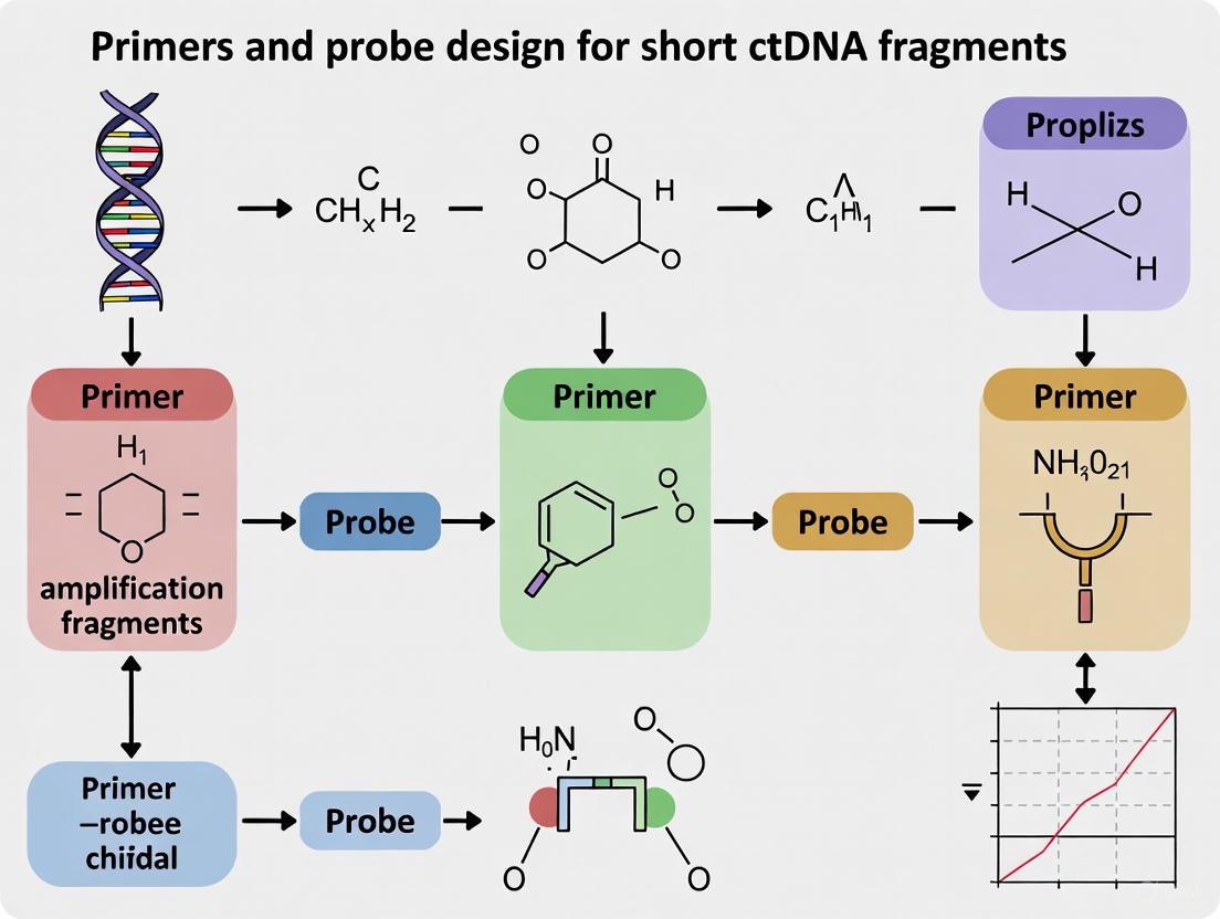
Precision Design of Primers and Probes for Short ctDNA Fragments: A Guide for Sensitive Liquid Biopsy Assays

Abstract

The analysis of circulating tumor DNA (ctDNA) through liquid biopsy has transformed oncology, enabling non-invasive cancer monitoring, therapy response assessment, and minimal residual disease detection. A central challenge in this field is the inherently short and fragmented nature of ctDNA, which often constitutes less than 1% of total cell-free DNA. This article provides a comprehensive guide for researchers and drug development professionals on designing primers and probes specifically optimized for these short ctDNA fragments. We cover the foundational biology of ctDNA fragmentation, detailed methodological strategies for PCR- and NGS-based assay design, troubleshooting for common pitfalls like false positives from clonal hematopoiesis, and rigorous validation frameworks. By focusing on these core aspects, the content aims to empower scientists to develop highly sensitive and specific liquid biopsy assays, thereby accelerating the translation of ctDNA analysis into clinical practice and drug development pipelines.

Understanding ctDNA Biology: Why Fragment Size Matters for Assay Design

Biological Foundations of ctDNA

What are the primary mechanisms of ctDNA release into circulation?

Circulating tumor DNA (ctDNA) is released into the bloodstream through several distinct biological processes, each imparting unique characteristics to the DNA fragments.

• Apoptosis (Programmed Cell Death): This is considered a major source of ctDNA. During apoptosis, caspase-activated DNases systematically cleave DNA into small, regular fragments. These fragments are typically wrapped around nucleosomes, resulting in a peak size of approximately 167 base pairs (bp), which corresponds to the length of DNA around one nucleosome (147 bp) plus a linker DNA (20 bp) [1] [2] [3]. The fragmentation follows a characteristic ladder-like pattern on gel electrophoresis.

• Necrosis (Unprogrammed Cell Death): This process occurs in response to adverse tumor conditions like hypoxia and nutrient depletion. Necrosis leads to cellular swelling and membrane rupture, resulting in the random and passive release of cellular contents. The DNA fragments from necrosis are typically larger and more heterogeneous, often exceeding 200 bp and sometimes reaching many kilobase pairs in size [2] [3].

• Active Secretion: Viable tumor cells can also actively release DNA through extracellular vesicles (EVs), such as exosomes and microvesicles [3]. The DNA associated with larger vesicles (100 nm to 1 μm) appears to be enriched with smaller fragments (<200 bp), while small EVs (30-150 nm) can carry DNA that is useful for mutation detection in early-stage cancer [3].

Table 1: Characteristics of ctDNA from Different Release Mechanisms

Release Mechanism	Primary Fragment Size	Fragmentation Pattern	Key Biological Triggers
Apoptosis	~167 bp (mononucleosomal)	Regular, ladder-like pattern	Programmed cell death, caspase activation [2]
Necrosis	>200 bp (often much larger)	Random, heterogeneous	Hypoxia, metabolic stress, inflammation [2] [3]
Active Secretion	Variable, often <200 bp	Varies with vesicle type	Cellular communication, viable cell release [3]

How do ctDNA fragment characteristics influence primer and probe design?

The unique size profile of ctDNA, particularly its short fragment length, has direct implications for the design of PCR primers and probes for detection assays.

• Amplicon Length: Given that ctDNA fragments are predominantly shorter than 200 bp, the ideal amplicon length for detection assays is typically 70-150 bp [4]. This ensures efficient amplification of the target ctDNA while avoiding amplification of longer, non-tumor cfDNA fragments.

• Assay Positioning: Designing assays to target shorter amplicons can enhance the sensitivity for detecting ctDNA. Research indicates that shorter fragments (<100 bp) may be enriched with tumor-derived genomic alterations [3].

• GC Content and Melting Temperature (Tm): Primers should have a GC content of 35-65% (ideal 50%) and a Tm of 60-64°C (ideal 62°C). The Tm of the forward and reverse primers should not differ by more than 2°C [4]. Probes should have a Tm 5-10°C higher than the primers to ensure they bind before the primers during the annealing step [4].

Troubleshooting Guide: Common ctDNA Experimental Challenges

Low signal intensity in fragment analysis

Problem: The signal from the sample is low, but the internal size standard signal is normal [5].

Solutions:

• Optimize PCR Conditions: Increase the amount of DNA template, adjust primer concentrations, or increase the number of PCR cycles [5].
• Check Primer Quality: If PCR products are visible on an agarose gel but not on the capillary electrophoresis instrument, the issue may be with the fluorescently labeled primer. Re-synthesizing the primer is recommended [5].
• Verify Sample Purity: The quality and method of DNA purification can significantly affect results. Select a purification method appropriate for your sample source and storage conditions [5].

Off-scale or saturated data

Problem: Peaks appear flat on top, indicating the signal is too high and saturating the detector [5].

Solutions:

• Dilute PCR Product: Further dilute the PCR product before injection. For instance, if using a 1:2 dilution, try 1:4 or 1:5 [5].
• Reduce Injection Time: Decrease the injection time in the instrument run module [5].
• Adjust Template Input: Reduce the amount of DNA template in the PCR reaction [5].

Detection of primer dimers and small artifacts

Problem: Small peaks appear before the 50 bp fragment, indicating the presence of primer dimers or excess fluorescently labeled primers [5].

Solutions:

• Optimize Primer Design: Screen primers for self-dimers and hairpins using tools like the OligoAnalyzer Tool. The ΔG value for any secondary structures should be weaker (more positive) than -9.0 kcal/mol [4].
• Purify PCR Product: Perform PCR purification to remove excess primers and small artifacts before capillary electrophoresis [5].

Experimental Workflow for ctDNA Analysis

Research Reagent Solutions

Table 2: Essential Reagents and Kits for ctDNA Research

Reagent/Kits	Primary Function	Key Considerations for ctDNA Work
Cell-Stabilization Blood Collection Tubes (e.g., Streck BCT)	Preserves blood sample integrity	Prevents white blood cell lysis during storage, reducing wild-type DNA contamination [1].
cfDNA Extraction Kits (e.g., QIAamp Circulating Nucleic Acid Kit)	Isolation of cell-free DNA from plasma	Optimized for low concentration, fragmented DNA; carrier RNA is often omitted [6].
Unique Molecular Identifiers	Tags individual DNA molecules pre-amplification	Essential for error correction in NGS; helps distinguish true mutations from PCR/sequencing errors [7].
Double-Quenched Probes (e.g., with ZEN/TAO)	Detection in qPCR/ddPCR	Provide lower background and higher signal-to-noise ratio, crucial for detecting low VAF targets [4].

Frequently Asked Questions (FAQs)

What is the difference between cfDNA and ctDNA?

Cell-free DNA (cfDNA) is a broad term for DNA freely circulating in the bloodstream, originating from various cell types, predominantly hematopoietic cells. Circulating tumor DNA (ctDNA) is a specific fraction of cfDNA that is derived from tumor cells and carries tumor-specific genetic alterations [1] [2].

Why is blood processing time critical for ctDNA analysis?

If blood collected in EDTA tubes is not processed promptly (within 2-4 hours), white blood cells begin to lyse, releasing large quantities of wild-type genomic DNA into the sample. This dilutes the ctDNA fraction, making detection of low-frequency mutations more difficult [1]. The use of cell-stabilization tubes can extend this processing window.

How does ctDNA fragment size inform assay design?

The nucleosomal footprint of ctDNA results in a characteristic fragment size distribution. Designing assays to target shorter amplicons (70-150 bp) can improve detection sensitivity by specifically amplifying the ctDNA fraction. Furthermore, in silico or physical size-selection of short fragments (<150 bp) can enrich for tumor-derived content [1].

What are the key factors affecting the limit of detection in ctDNA assays?

The limit of detection is influenced by:

• Variant Allele Frequency: The fraction of mutant alleles in the total cfDNA.
• Sequencing Depth: The number of unique reads covering a genomic position.
• Input DNA Mass: The total amount of cfDNA available for analysis, which determines the absolute number of mutant DNA molecules present [7].
• Assay Background Error Rate: The frequency of errors introduced during library preparation and sequencing.

FAQs: Fundamentals of ctDNA Size Profiling

Q1: Why is the 100-150 bp size range particularly significant for ctDNA analysis?

Circulating tumor DNA fragments are consistently shorter than cell-free DNA (cfDNA) from healthy cells. While healthy cfDNA shows a strong peak at approximately 167 bp (corresponding to DNA protected by a nucleosome), ctDNA is enriched in fragments ranging from 90-150 bp, with some studies noting enrichment in the 126-135 bp range and even 240-324 bp fragments [8] [9]. This size difference provides a physical characteristic that can be exploited to separate tumor-derived DNA from the normal background, significantly improving detection sensitivity [10] [11].

Q2: What is the biological rationale behind the shorter length of ctDNA?

The non-random fragmentation pattern of cfDNA is thought to reflect the chromatin structure of the cells from which it originated [11]. Tumor cells have different chromatin packaging and epigenetic states compared to healthy cells. The enrichment of shorter fragments in ctDNA is likely a result of these distinct epigenetic landscapes and differences in the cell death processes (e.g., apoptosis vs. necrosis) that release DNA into the bloodstream [11] [9].

Q3: How does fragment size selection impact the detection of low-frequency variants?

Enriching for shorter fragments can significantly improve the detection of variants with low allele frequencies. Plasmid simulation experiments have demonstrated that methods selecting for shorter fragments can substantially improve ctDNA detection in samples with low variant allele frequency (VAF) [8]. In real-world clinical samples, this approach increases the chance of capturing alteration reads from short fragments, which is crucial for detecting low-frequency mutations [8].

Troubleshooting Guides

Issue 1: Inadequate Enrichment of Short ctDNA Fragments

Potential Causes and Solutions:

• Cause: Incorrect bead-to-sample ratio during size selection.
  • Solution: For single-strand DNA (ssDNA) library preparation, using a large proportion of magnetic beads (e.g., 1.8x post-extension, 1.6x post-ligation, and 1.6x post-PCR cleanup) has been shown to better recover fragments longer than 40 bp and enrich the shorter cfDNA fraction [8].
• Cause: Standard double-strand DNA (dsDNA) library prep protocols may under-represent short fragments.
  • Solution: Consider switching to a single-strand DNA (ssDNA) library preparation method. Studies show that ssDNA libraries are particularly useful for managing degraded and fragmented DNA and result in higher ctDNA content associated with shorter insert sizes [8].
• Cause: Inefficient target capture due to poor probe design.
  • Solution: For targeted sequencing, ensure that capture probes are designed to effectively hybridize with the shorter fragment population. Using tumor-informed panels with high tiling density (e.g., 1x, 2x, or 3x) can improve the capture efficiency of ctDNA-derived fragments [12].

Issue 2: Low Concordance Between ctDNA and Tumor Tissue Genotyping

Potential Causes and Solutions:

• Cause: Spatial tumor heterogeneity, where a single tissue biopsy does not capture the complete genomic profile of the tumor.
  • Solution: Recognize that liquid biopsy can capture DNA shed from multiple tumor sites. A degree of discordance is expected and may provide a more comprehensive view of the disease [13]. Use fragmentomics as a complementary, tumor-agnostic method that does not rely solely on specific genetic alterations [14] [11].
• Cause: Low tumor DNA shedding, leading to very low ctDNA fraction in plasma.
  • Solution: Apply in-silico bioinformatic enrichment after sequencing. The CISBEP process, which selects sequencing reads based on fragment size features (e.g., 126-135 bp), can increase the effective tumor fraction for analysis, improving the detection of copy number alterations [9].

Issue 3: High Background Noise in Fragmentomic Data

Potential Causes and Solutions:

• Cause: Background cfDNA from hematopoietic cells diluting the tumor-derived signal.
  • Solution: Integrate multiple fragmentation features beyond just size. Studies show that combining fragment size with other features like the genomic position of fragment ends relative to nucleosomes and the presence of specific DNA end motifs can result in a higher enrichment of ctDNA compared to using fragment size selection alone (providing an additional 7-25% enrichment) [9].
• Cause: False positive variants caused by clonal hematopoiesis (CHIP).
  • Solution: Always sequence a matched buffy coat (white blood cell) control from the same blood draw. This allows for the identification and subtraction of somatic variants arising from blood cells, which is critical for reducing false positives [15] [16].

Quantitative Data on ctDNA Fragment Sizes

The following table summarizes key quantitative findings from recent studies on ctDNA fragment size distributions.

Size Range (bp)	Observed Enrichment / Characteristic	Clinical / Experimental Context	Citation
90 - 150 bp	Obtained shorter cfDNA; improved detection of low-VAF variants.	ssDNA library prep with large bead ratio in advanced cancers (NSCLC, ESCC, etc.).	[8]
100 - 150 bp	Typically shorter than non-tumor cfDNA; a key biomarker.	General characteristic of ctDNA used for liquid biopsy monitoring.	[12]
126 - 135 bp	28% - 87% ctDNA enrichment.	In-silico size selection in high-grade serious ovarian cancer (HGSOC).	[9]
< 150 bp	Proportion of short fragments consistently higher in Ewing sarcoma vs. healthy controls.	Global fragment-size analysis in pediatric sarcomas via WGS.	[11]
240 - 324 bp	28% - 159% ctDNA enrichment.	In-silico selection of di-nucleosome-sized fragments in HGSOC.	[9]
~167 bp	Peak for healthy cfDNA; ctDNA shows a shift away from this peak.	Corresponds to DNA wrapped around a nucleosome plus linker; used as a reference.	[8] [11]

Experimental Workflow & Signaling Pathways

ctDNA Short-Fragment Enrichment Workflow

The diagram below outlines a core experimental protocol for enriching and analyzing short ctDNA fragments, synthesizing methods from the cited literature.

Integrating Fragmentomics into ctDNA Analysis

This diagram illustrates the logical relationship between the biological origins of cfDNA/ctDNA, their measurable fragmentomic features, and the resulting clinical applications.

The Scientist's Toolkit: Research Reagent Solutions

Essential Material / Reagent	Function in ctDNA Size Profiling	Specific Examples / Notes
Specialized Blood Collection Tubes	Stabilizes blood cells to prevent genomic DNA contamination that would dilute the ctDNA signal.	Streck Cell-Free DNA BCT Tubes, PAXgene Blood ccfDNA Tubes [13] [14].
ssDNA Library Prep Kit	More efficient at capturing short, fragmented DNA compared to standard dsDNA kits.	Accel-NGS 1S Plus DNA Library Kit (Swift Biosciences) [8].
Magnetic Beads	Used for size selection and clean-up steps. A large bead-to-sample ratio enriches for shorter fragments.	VAHTS DNA Clean Beads; used at ratios of 1.8x, 1.6x, and 1.6x in key steps [8].
Tumor-Informed Panels	Custom oligonucleotide probes designed to track 20-100 patient-specific mutations identified from prior tumor sequencing.	xGen (IDT) or Twist panels; high tiling density (2x, 3x) improves capture [12].
Unique Molecular Identifiers (UMIs)	Short DNA barcodes ligated to each original DNA molecule before PCR to correct for amplification errors and duplicates.	Integrated into library prep adapters; essential for achieving error rates < 10⁻⁵ [12].
Bioinformatic Tools	Software for analyzing fragmentation patterns, performing in-silico size selection, and calling low-frequency variants.	ichorCNA (for copy number analysis), LIQUORICE (for chromatin signatures), umiVar (for UMI-based variant calling) [11] [12] [9].

The Biological Half-Life of ctDNA and Its Implications for Real-Time Monitoring

Frequently Asked Questions (FAQs)

Q1: Why is the short biological half-life of ctDNA critical for monitoring cancer therapy? The short half-life of circulating tumor DNA (ctDNA), estimated between 16 minutes and 2.5 hours, allows it to serve as a nearly real-time indicator of tumor dynamics [17] [18]. This rapid turnover means changes in tumor burden, such as response to therapy or the emergence of resistance, are quickly reflected in ctDNA levels. This enables much faster assessment of treatment efficacy compared to traditional imaging, which can take weeks or months to show anatomical changes [18].

Q2: What is the primary challenge when designing primers and probes for short ctDNA fragments? The foremost challenge is that ctDNA is highly fragmented, with sizes typically ranging from 20 to 220 base pairs and a peak around 167 bp (the length of DNA wrapped around a single nucleosome) [19]. Primer and probe sets must be designed to efficiently target these short, fragmented sequences while avoiding non-specific amplification of the much larger background of wild-type cell-free DNA.

Q3: How can pre-analytical variables lead to false-negative ctDNA results? Pre-analytical errors are a major source of false negatives. Key issues include:

• Sample Processing Delays: Using conventional EDTA blood collection tubes but exceeding the 2-6 hour processing window at 4°C, leading to white blood cell lysis and contamination of the sample with genomic DNA [20].
• Improper Centrifugation: Failure to use a two-step centrifugation protocol can leave cellular debris or intact cells in the plasma, which later lyse and dilute the tumor-derived signal with wild-type DNA [19] [20].
• Inadequate Blood Volume: Drawing less than 10 mL of blood may not provide a sufficient number of mutant DNA fragments for reliable detection, especially in early-stage disease where the ctDNA fraction can be below 0.1% [7].

Q4: What strategies can improve the detection of low-frequency ctDNA variants? To detect variants with very low variant allele frequencies (VAFs), consider these approaches:

• Increase Sequencing Depth: Detecting a variant at a 0.1% VAF with 99% confidence requires a sequencing depth of approximately 10,000x [7].
• Incorporate Unique Molecular Identifiers (UMIs): Barcoding individual DNA molecules before PCR amplification allows bioinformatics tools to identify and correct for sequencing errors, distinguishing true low-frequency variants from technical artifacts [7] [18] [21].
• Utilize Error-Corrected NGS Methods: Techniques like CyclomicsSeq or Duplex Sequencing create consensus sequences from multiple reads of a single original DNA molecule, reducing error rates and enabling detection of variants at frequencies as low as 0.02% [22].

Troubleshooting Common Experimental Issues

Table 1: Troubleshooting Low ctDNA Yield or Quality

Problem	Potential Cause	Recommended Solution
High wild-type DNA background	Blood cell lysis due to delayed processing or use of inappropriate collection tubes.	For EDTA tubes, process plasma within 2-6 hours of draw. For longer stability, use specialized cell-stabilizing tubes (e.g., Streck, PAXgene) that allow storage for up to 3-7 days at room temperature [19] [20].
Low variant detection sensitivity	Input ctDNA mass is too low, providing an insufficient number of mutant genome equivalents.	Ensure a sufficient volume of blood is collected (e.g., 2x10 mL tubes). The input for library preparation should be at least 60 ng of cfDNA to achieve the high coverage needed for low-VAF detection [7].
Inconsistent results between replicates	Inefficient removal of PCR duplicates during bioinformatics analysis.	Implement a UMI-based deduplication pipeline in your NGS workflow to accurately count original DNA molecules and reduce quantitative bias [7].

Table 2: Quantitative Data for Experimental Design

Parameter	Typical Range or Value	Implication for Experimental Design
ctDNA Half-Life	16 min - 2.5 hours [17] [18]	Enables real-time monitoring; frequent sampling (e.g., pre-dose, 24h post-treatment) can capture rapid dynamics.
ctDNA Fragment Size	20-220 bp, peak at ~167 bp [19]	Design PCR amplicons to be short (<150 bp) to ensure efficient amplification of the target ctDNA.
Limit of Detection (LoD)	0.02% - 0.5% VAF [7] [22] [23]	Choose a sequencing technology with a LoD suited to your expected ctDNA fraction (lower for MRD, higher for advanced disease).
Required Sequencing Depth	~10,000x for 0.1% VAF [7]	Plan sequencing capacity and multiplexing accordingly to achieve the necessary depth for your sensitivity goals.

Essential Protocols and Workflows

Protocol 1: Optimal Plasma Processing for ctDNA Analysis

This protocol is critical for preserving ctDNA integrity and minimizing contamination [19] [20].

• Blood Collection: Draw blood into appropriate tubes. For EDTA tubes, proceed immediately. For specialized BCTs (e.g., Streck), note the stability window.
• First Centrifugation: Centrifuge at 1200–2000 × g for 10 minutes at 4°C to separate plasma from blood cells.
• Plasma Transfer: Carefully transfer the supernatant plasma to a new tube, taking extreme care not to disturb the buffy coat layer.
• Second Centrifugation: Centrifuge the plasma at 12,000–16,000 × g for 10 minutes at 4°C to pellet any remaining cellular debris.
• Plasma Storage: Aliquot the cleared plasma and store at -80°C to prevent degradation and avoid freeze-thaw cycles.
• cfDNA Extraction: Use a column-based or magnetic bead-based extraction kit optimized for cfDNA (e.g., QIAamp Circulating Nucleic Acid Kit).

Protocol 2: Wet-Lab Workflow for Error-Corrected NGS

This workflow outlines the steps for highly sensitive ctDNA detection using UMI-based NGS [7] [22].

Protocol 3: Bioinformatic Pipeline for Sensitive Variant Calling

This logical workflow follows the wet-lab protocol to identify true low-frequency variants [7] [22].

The Scientist's Toolkit: Essential Research Reagents

Table 3: Key Reagents for ctDNA Research

Reagent / Kit	Function	Key Consideration
Cell-Free DNA Blood Collection Tubes (e.g., Streck BCT)	Prevents white blood cell lysis, preserving cfDNA profile for up to 7 days at room temperature [19] [20].	Essential for multi-center studies or when immediate processing is not feasible.
cfDNA Extraction Kits (e.g., QIAamp Circulating Nucleic Acid Kit)	Isletes high-quality, short-fragment cfDNA from plasma while removing PCR inhibitors [19] [20].	Column-based kits often provide higher yields than magnetic bead-based methods.
UMI Adapters	Short nucleotide barcodes ligated to each DNA fragment prior to PCR amplification [7] [22].	Allows for bioinformatic correction of PCR and sequencing errors, crucial for low-VAF detection.
Targeted NGS Panels	Multiplex PCR or hybrid-capture panels designed to amplify cancer-associated genes from small amounts of input DNA [17] [18].	Panels should be designed with short amplicons (<150 bp) to match the fragmented nature of ctDNA.
Droplet Digital PCR (ddPCR) Assays	Absolute quantification of specific mutations without the need for standard curves; offers high sensitivity [17] [18].	Ideal for longitudinal tracking of a known mutation but low-throughput for discovering new variants.

Circulating tumor DNA (ctDNA) refers to the fragmented DNA released into the bloodstream by cancerous cells and tumors. The central challenge in liquid biopsy is that ctDNA often represents a very small fraction of the total cell-free DNA (cfDNA), the majority of which originates from the natural death of hematopoietic cells [24] [25] [26]. This low abundance makes the tumor-derived mutations exceptionally difficult to detect, presenting a significant technical hurdle for using ctDNA as a reliable clinical marker [24]. The term "Tumor Fraction" (TF) quantifies this proportion, representing the amount of circulating tumor DNA as a fraction of total cell-free DNA in a blood sample [26]. Accurate assessment of this fraction is critical for interpreting test results, especially negative findings.

Key Concepts & Biological Principles

What are ctDNA and cfDNA?

• Cell-free DNA (cfDNA): A mix of DNA fragments found in the bloodstream, shed by various cells in the body.
• Circulating Tumor DNA (ctDNA): The subset of cfDNA that originates specifically from tumor cells. These fragments are typically shorter than 200 nucleotides and carry the genetic mutations of the tumor they came from [25] [27].

The Size Difference Advantage

A key biological property that can be leveraged to overcome the challenge of low abundance is fragment length. Multiple studies have consolidated the finding that ctDNA fragments are generally shorter than non-malignant cfDNA fragments [24] [14]. One study showed that mutant alleles (ctDNA) occur more commonly at a shorter fragment length (134–144 bp) than the wild-type allele (165 bp) [24]. This size difference provides a critical foundation for designing more sensitive detection assays.

Experimental Protocols & Methodologies

Protocol: Optimizing Detection via Short Amplicon Sequencing

This protocol is designed to enhance the detection of low-abundance ctDNA by exploiting its shorter fragment length [24].

• Objective: To investigate how amplicon length impacts the capacity to detect ctDNA in plasma samples.
• Materials:
  • Plasma DNA samples (e.g., from pancreatic cancer patients with known KRAS mutations).
  • Primers designed for a target region (e.g., KRAS codon 12).
  • Resources for ultra-deep sequencing (e.g., Ion Proton System).
• Procedure:
  • Primer Design: Design multiple primer sets to generate amplicons of varying lengths (e.g., 57 bp, 79 bp, 167 bp, and 218 bp) covering the same target mutation hotspot.
  • Independent PCR Amplification: Perform separate PCR amplifications for each amplicon size using the same amount of input cfDNA (e.g., 2 ng) and identical experimental conditions.
  • Library Preparation & Barcoding: Prepare barcoded libraries from each amplification product.
  • Ultra-deep Sequencing: Sequence the libraries using a high-throughput platform to achieve ultra-deep coverage.
  • Bioinformatic Analysis: Map reads to the reference genome and calculate the Mutant Allelic Fraction (MAF) for each amplicon size. MAF is the proportion of sequencing reads that contain the mutant allele versus the wild-type allele.
• Expected Outcome: Shorter amplicons (e.g., 57 bp and 79 bp) will yield a significantly higher MAF and a greater proportion of samples with detectable mutations compared to longer amplicons (e.g., 167 bp and 218 bp) [24].

Protocol: Fragmentomic Analysis for Tumor Agnostic Monitoring

This protocol uses a qPCR-based approach to quantify size-distributed cfDNA fragments, generating a "Progression Score" for monitoring treatment response in advanced cancer [14].

• Objective: To monitor disease progression in stage IV cancer patients by analyzing cfDNA fragment size patterns.
• Materials:
  • Plasma samples collected in Streck cfDNA BCT tubes.
  • qPCR system and reagents.
  • Primers targeting multi-copy retrotransposon elements (e.g., ALU).
• Procedure:
  • Plasma Separation: Use a two-step centrifugation protocol to isolate plasma from peripheral blood.
  • cfDNA Extraction: Extract cfDNA from a fixed volume of plasma (e.g., 4 mL).
  • Multi-size qPCR Quantification: Perform qPCR assays targeting specific repetitive elements (e.g., ALU) to quantify cfDNA fragments of different size thresholds (e.g., >80 bp, >105 bp, and >265 bp).
  • Calculate Progression Score (PS): Integrate the quantitative data from the different fragment sizes into a model that outputs a Progression Score from 0 to 100. A high score indicates probable disease progression.
• Expected Outcome: The PS can predict radiographic progression with high accuracy as early as 2-3 weeks after treatment initiation, allowing for rapid assessment of therapy efficacy [14].

Troubleshooting Guides & FAQs

FAQ 1: Why is my ctDNA assay failing to detect mutations in a patient with confirmed advanced cancer?

• Potential Cause: Low tumor fraction (TF). The amount of ctDNA in the total cfDNA is below the detection limit of your assay.
• Solution:
  • Target Short Amplicons: Re-design your assay to target amplicons less than 80 bp to enrich for the shorter ctDNA fragments [24].
  • Check TF: If using a commercial test like FoundationOneLiquid CDx, check the reported ctDNA tumor fraction. A low TF (<1%) indicates that a negative result may be due to low ctDNA abundance rather than the true absence of alterations. In such cases, a tissue biopsy is recommended for confirmation [26].
  • Pre-analytical Factors: Ensure proper blood sample collection and processing (e.g., using Streck tubes and processing within 72 hours) to prevent white blood cell lysis that dilutes the ctDNA signal [14] [28].

FAQ 2: How can I increase confidence in a negative liquid biopsy result?

• Solution: Incorporate tumor fraction assessment. A negative result from a high-quality assay is more reliable if the TF is high (e.g., ≥1%), suggesting the assay had sufficient material to detect mutations if they were present. Conversely, a negative result with a low TF should be interpreted with caution [26].

FAQ 3: My NGS analysis pipeline for ctDNA failed. What are the first steps to debug?

• Solution:
  • Check Log Files: Navigate to the analysis output directory and review the pipeline_trace.txt and step-specific log files in the Logs_Intermediates folder for error messages [29].
  • Validate Sample Sheet: Ensure the sample sheet is in the correct format (v2 for DRAGEN TSO 500), contains unique sample IDs, and uses valid index combinations for your assay [29].
  • Verify Input Files: Confirm that BCL or FASTQ input files are in the correct location and are not corrupted [29].

Data Presentation: Quantitative Impact of Amplicon Size

The following table summarizes the quantitative impact of amplicon size on ctDNA detection sensitivity, based on a study screening KRAS mutations in pancreatic cancer plasma samples [24].

Table 1: Impact of Amplicon Size on KRAS Mutation Detection in Plasma

Amplicon Size	Average Mutant Allelic Fraction (MAF)	Relative MAF Reduction (vs. 57 bp)	Proportion of Cases with Detectable Mutation
57 bp	Baseline	-	100% (Reference)
79 bp	Lower than 57 bp	Significant	High (Similar to 57 bp)
167 bp	Significantly Lower	Significant	Reduced
218 bp	Lowest	4.6-fold (95% CI: 2.6-8.1)	~50% (Half of 57 bp detection rate)

The Scientist's Toolkit: Research Reagent Solutions

Table 2: Essential Reagents and Kits for ctDNA Research

Item	Function/Application	Example Product
Cell-Free DNA Blood Collection Tubes	Stabilizes blood cells to prevent genomic DNA contamination during transport. Critical for preserving the true cfDNA profile.	Cell-Free DNA BCT (Streck) [14] [28]
Plasma cfDNA Purification Kit	Extracts cfDNA from plasma samples with high efficiency and low contamination.	Plasma cfDNA Purification Kit (Concert) [28]
Library Preparation Kit	Prepares sequencing libraries from low-input, fragmented cfDNA.	KAPA HyperPrep Kit (KAPA Biosystems) [28]
Ultra-deep Sequencing Platform	Provides the high sequencing depth required to detect low-frequency mutations in ctDNA.	Ion Proton System (Thermo Fisher) [24]; MGISEQ-2000 (MGI) [28]

Visualization of Workflows and Concepts

Experimental Workflow for ctDNA Analysis

This diagram illustrates the core workflow for analyzing ctDNA, from sample collection to data interpretation, highlighting key steps to address low abundance.

Decision Pathway for Negative Liquid Biopsy Results

This flowchart provides a logical framework for researchers to follow when confronted with a negative liquid biopsy result, emphasizing the critical role of tumor fraction.

Linking ctDNA Shedding to Tumor Burden, Type, and Vascularity

FAQs on ctDNA Biology and Analysis

1. Why does my ctDNA assay sometimes yield false-negative results, even with a known metastatic tumor? False-negative results can occur due to biological and technical factors. Biologically, the shedding of ctDNA into the bloodstream is not uniform across all tumors. Key factors influencing shedding include:

• Tumor Genotype: The genetic makeup of the tumor significantly impacts shedding. For instance, EGFR-mutant non-small cell lung cancers (NSCLC) have been shown to shed less ctDNA compared to KRAS or TP53 mutant NSCLC, independent of tumor burden [30].
• Anatomic Location: Tumors in certain body sites may release lower amounts of ctDNA into the peripheral circulation. For primary brain tumors, cerebrospinal fluid (CSF) is a more sensitive source of ctDNA than blood [31].
• Low Shedding Phenotype: Some metastatic tumors intrinsically release very low amounts of ctDNA, a phenomenon not yet fully understood [31]. Technically, false negatives can stem from a low volume of plasma analyzed, which limits the number of genome copies available for detection, especially for subclonal mutations [31].

2. How does tumor vascularity influence the amount of ctDNA I can detect in a blood sample? Increased tumor vascularity facilitates the trafficking of cell-free DNA into the circulation. A higher degree of vascularization, often coupled with greater depth of tumor invasion, leads to greater ctDNA levels quantified by the circulating tumor allele fraction (cTAF) [32]. Clinically significant, aggressive cancers, which are often highly vascularized, show higher cTAF than indolent cancers at the same stage [32].

3. My ctDNA levels and imaging results seem to disagree. Which should I trust? Discrepancies can occur and provide important biological and clinical insights. ctDNA levels reflect the total metabolic tumor burden and cellular turnover, while imaging (e.g., CT) measures anatomic volume [30]. A moderate but significant correlation exists between ctDNA variant allele frequency (VAF) and imaging measures like CT volume or metabolic tumor volume (MTV) [30]. However, genotype-specific shedding differences can weaken this correlation. Furthermore, ctDNA can detect molecular progression or response weeks before changes are visible on a scan, making it a leading indicator of disease status [6] [33]. In cases of discrepancy, it is crucial to consider the tumor genotype and combine both modalities for a comprehensive assessment.

4. Are there tumor-agnostic methods to monitor tumor burden via liquid biopsy? Yes, fragmentomics is an emerging tumor-agnostic approach. It does not rely on detecting specific mutations but instead analyzes the patterns of cfDNA fragmentation. Cancer-derived cfDNA fragments tend to be shorter and display distinct size distributions and end-motif preferences compared to healthy cfDNA [6]. One such assay quantifies specific cfDNA fragment sizes via qPCR to generate a "Progression Score" (PS) that correlates with radiographic progression, independent of the tumor's genomic profile [6]. This can be particularly useful for tumors without known recurrent mutations.

Troubleshooting Common Experimental Challenges

Challenge	Possible Causes	Proposed Solutions
Low ctDNA Signal	• Low-shedding tumor genotype (e.g., EGFR+ NSCLC) [30]• Early-stage or low-burden disease [33]• Inefficient cfDNA extraction	• Pre-analytical assessment: Use imaging to confirm tumor burden [30].• Analytical enhancement: Employ patient-specific, tumor-informed panels to track multiple mutations [33].• Technical optimization: Use ultra-deep sequencing methods and size-selection protocols for short cfDNA fragments [31].
Discordant Tissue & Plasma Genotyping	• Spatial tumor heterogeneity [31]• Clonal evolution post-biopsy [31]• Technical false positives from NGS errors [31]	• Biological interpretation: Discordance may reveal heterogeneity or evolution.• Technical control: Use error-suppression strategies (e.g., molecular barcodes, unique molecular identifiers - UMIs) and validate with orthogonal techniques (e.g., ddPCR) [31] [33].
High Background Noise in NGS	• Clonal hematopoiesis• Errors from library preparation and amplification [31]	• Wet-lab refinement: Implement duplex sequencing with UMIs to create consensus reads [33].• Bioinformatic filtering: Apply robust bioinformatic pipelines to distinguish true somatic variants from artifacts [31].

Key Quantitative Relationships: Tumor Burden & ctDNA

The table below summarizes key quantitative correlations observed in clinical studies, which are essential for interpreting ctDNA data.

Table 1: Correlations between ctDNA Levels and Tumor Burden Metrics

Tumor Burden Metric	Correlation with ctDNA (Spearman's rho)	P-value	Context & Notes	Source
CT Tumor Volume	0.34	p ≤ 0.0001	Moderate correlation across NSCLC cohort.	[30]
Metabolic Tumor Volume (MTV)	0.36	p = 0.003	Stronger correlation in a subset with PET/CT imaging.	[30]
CT Tumor Volume (Localized RMS)	0.70 (ctDNA level)	p = 0.03	Pre-treatment correlation in pediatric Rhabdomyosarcoma.	[33]
cfDNA Concentration (Localized RMS)	0.83 (cfDNA level)	p = 0.01	Pre-treatment correlation in pediatric Rhabdomyosarcoma.	[33]

Table 2: Genotype-Specific Differences in ctDNA Shedding

Genotype	Correlation with CT Volume (rho)	P-value	Context & Notes	Source
KRAS mutant	0.56	p ≤ 0.001	Strongest correlation between tumor burden and ctDNA shedding.	[30]
TP53 mutant	0.43	p ≤ 0.0001	Intermediate correlation.	[30]
EGFR mutant	0.24	p = 0.077	Weakest and non-significant correlation. Shedding is also influenced by copy number gain.	[30]

Detailed Experimental Protocols

Protocol 1: Establishing a Correlation Between ctDNA VAF and Radiographic Tumor Burden

This protocol is adapted from a retrospective study in NSCLC [30].

1. Sample and Data Collection:

• Cohort: Identify patients with advanced-stage cancer (e.g., NSCLC) prior to initiating a new line of therapy.
• Blood Collection: Draw blood into cell-free DNA BCT tubes (e.g., Streck). Process plasma via a two-step centrifugation protocol (e.g., 1600× g for 10 min, then 16,000× g for 10 min) within a strict time window (e.g., <120 hours post-draw) to prevent cfDNA degradation [6]. Store plasma at -80°C.
• Imaging: Obtain CT (and if available, 18F-FDG PET-CT) scans within 30 days of blood draw.

2. Laboratory Analysis:

• cfDNA Extraction: Extract cfDNA from 1-5 mL of plasma using a commercial kit (e.g., QIAamp Circulating Nucleic Acid Kit).
• ctDNA Sequencing: Perform next-generation sequencing using a targeted or comprehensive NGS panel (e.g., Guardant360). Define the ctDNA level for each sample as the maximum variant allele frequency (VAF) detected among all somatic alterations.

3. Radiographic Quantification:

• CT Volume: Use semi-automated contouring software (e.g., syngo.via) to calculate total tumor volume in cm³.
• PET Parameters: For PET-CT, calculate the Metabolic Tumor Volume (MTV) and Total Lesion Glycolysis (TLG) using dedicated software (e.g., MIM Software).

4. Data Analysis:

• Use non-parametric statistics (e.g., Spearman's rank correlation) to assess the relationship between the maximum ctDNA VAF and each radiographic measure of tumor burden (CT volume, MTV).
• Perform subgroup analysis based on major driver mutations (e.g., EGFR, KRAS, TP53).

Protocol 2: Ultrasensitive Monitoring Using Patient-Specific Sequencing Panels

This protocol is ideal for tumors with high genetic heterogeneity, such as pediatric sarcomas [33].

1. Tumor and Normal Sequencing:

• Perform Whole Exome Sequencing (WES) or Whole Genome Sequencing (WGS) on tumor DNA and matched germline DNA (from leukocytes).

2. Panel Design and Validation:

• Variant Selection: Identify approximately 50-150 high-confidence, tumor-specific single nucleotide variants (SNVs) from WES. Select 10 SNVs with high VAF (>10%) for the final panel, prioritizing clonal, non-synonymous mutations in cancer-related genes.
• Primer Design: Design PCR primers for each selected SNV.
• In-silico Validation: Ensure selected SNVs are not in low-complexity regions and that primers are specific.

3. ctDNA Analysis:

• Library Preparation: Construct sequencing libraries from plasma cfDNA. The use of Unique Molecular Identifiers (UMIs) is critical for error correction.
• Deep Sequencing: Sequence the customized panel to a high median depth (>15,000x raw reads).
• Bioinformatic Processing: Generate consensus reads from UMI families to eliminate PCR and sequencing errors. A sample should be excluded if the total consensus reads are too low (e.g., <400).
• Quantification: Report ctDNA levels as Mutated Tumor Molecules per mL of plasma (MTM/mL).

The Scientist's Toolkit: Research Reagent Solutions

Table 3: Essential Materials for ctDNA Analysis

Item	Function/Benefit	Example Product/Catalog
Cell-Free DNA Blood Collection Tubes	Preserves blood sample integrity by stabilizing nucleated blood cells, preventing genomic DNA contamination and cfDNA degradation during transport.	Streck Cell-Free DNA BCT Tubes
Circulating Nucleic Acid Extraction Kit	Efficiently isolates short-fragment cfDNA from large-volume plasma samples.	QIAamp Circulating Nucleic Acid Kit (Qiagen)
Targeted NGS Panel	For mutation detection and quantification in a clinically validated, tumor-agnostic format. Covers a wide range of genes.	Guardant360
Unique Molecular Identifiers (UMIs)	Short random nucleotide sequences added to each DNA molecule before PCR. Allows bioinformatic correction of errors, enabling ultrasensitive detection.	Included in various commercial and custom NGS library prep kits

Experimental Workflow and Biological Pathways

ctDNA Analysis & Tumor Burden Correlation Workflow

Biological Determinants of ctDNA Shedding

Strategic Primer and Probe Design for Maximizing ctDNA Detection Sensitivity

The accurate detection and quantification of circulating tumor DNA (ctDNA) presents a significant challenge in molecular diagnostics. ctDNA fragments in blood plasma are notoriously short, often significantly shorter than the cell-free DNA (cfDNA) derived from healthy cells [34]. This fundamental characteristic dictates that assays designed for ctDNA research must be optimized for very short amplicons to maximize detection sensitivity and accuracy. The selection of an appropriate amplicon length is not merely a technical detail but a critical parameter that directly influences the efficiency, specificity, and overall success of qPCR and ddPCR assays in a liquid biopsy context. The need for short amplicons is particularly pronounced during the detection of minute amounts of ctDNA from limited plasma samples, where every molecule counts [34]. This guide provides a detailed framework for selecting optimal amplicon lengths, troubleshooting common issues, and implementing robust experimental protocols for ctDNA research.

FAQs on Amplicon Length Selection

What is the ideal amplicon length for a standard qPCR assay?

For standard quantitative PCR (qPCR), the recommended amplicon length typically falls within a 75–150 base pair (bp) range [35]. This size is considered optimal because shorter amplicons are amplified with higher efficiency due to a lower probability of polymerase errors and faster extension times [36] [4]. Amplicons within this range are most easily amplified using standard cycling conditions, providing a reliable balance between robust amplification and specific detection.

Why are even shorter amplicons critical for ctDNA detection?

ctDNA fragments found in blood plasma are often highly degraded and tend to be short [34]. Designing assays with amplicons under 100 bp is therefore crucial to ensure that the assay can amplify the degraded ctDNA templates. Using longer amplicons risks missing a significant fraction of the ctDNA molecules because the target sequence may be physically shorter than the amplicon length, leading to false negatives and a severe underestimation of ctDNA concentration. Techniques like PNB-qPCR (Pooled, Nested, WT-Blocking qPCR) leverage short amplicons to enable sensitive quantification of minute amounts of ctDNA from limited plasma samples [34].

Is there a trade-off between amplicon length and live/dead discrimination in viability assays?

Yes, this trade-off is a well-documented dilemma. In viability quantitative PCR (v-qPCR), which uses dyes like propidium monoazide (PMA) to distinguish DNA from membrane-compromised dead cells, amplicon length is a key factor [36]. Longer amplicons increase the probability that a viability dye molecule is bound to the DNA segment, thereby more effectively blocking its amplification and improving the distinction between live and dead cells. However, longer amplicons are amplified with lower qPCR efficiency. Research suggests a practical balance is achieved with amplicons between approximately 200 bp and 400 bp for v-qPCR, which provides good live/dead distinction while maintaining acceptable efficiency [36].

How does amplicon length affect PCR efficiency?

There is a strong negative correlation between amplicon length and PCR efficiency. Longer DNA sequences require more time for the polymerase to fully copy and have a higher chance of containing secondary structures or regions that are difficult to amplify (e.g., GC-rich regions). This can lead to increased cycle threshold (Cq) values and greater variation between replicates [36]. Consequently, shorter amplicons (e.g., 75-150 bp) are generally associated with near-optimal, high-efficiency amplification [4].

Troubleshooting Guide

The following table outlines common issues related to amplicon length and their potential solutions.

Problem	Potential Cause	Troubleshooting Recommendations
Low Amplification Efficiency/High Cq	Amplicon too long; poor polymerase processivity.	Redesign assay for a shorter amplicon (70–150 bp) [35] [4]. Verify polymerase is suitable for target length and increase extension time if necessary (1 min/kb rule of thumb) [35].
False Negative ctDNA Results	Amplicon length exceeds the size of degraded ctDNA fragments.	Design amplicons to be shorter than 100 bp to match the characteristic short length of ctDNA [34].
Poor Live/Dead Discrimination in v-qPCR	Amplicon is too short to allow sufficient viability dye binding.	Optimize amplicon length for a trade-off. A range of ~200–400 bp can increase Cq differences between live/dead cells while maintaining reasonable efficiency [36].
Non-Specific Amplification or Primer-Dimers	Amplicon is very short, and primers are poorly designed.	Optimize primer design to ensure specificity. Use hot-start DNA polymerases and optimize annealing temperature [37]. Check for primer-dimer formation with a dissociation curve [38].
Inconsistent Results (High Variation Between Replicates)	Very long amplicons leading to stochastic amplification failures.	Shorten the amplicon length. For long targets, ensure consistent template quality and increase polymerase concentration or switch to a high-processivity enzyme [37].

Experimental Protocol: Establishing a Short-Amplicon Assay

The following workflow, adapted from methodologies used in sensitive ctDNA detection, outlines the key steps for establishing a robust short-amplicon qPCR/ddPCR assay [34].

Step-by-Step Methodology

• Target Identification and Assay Definition: Clearly define the genomic target, such as a specific KRAS point mutation for ctDNA analysis [34]. Consult curated sequence databases (e.g., NCBI RefSeq) and use the specific accession number to ensure accuracy [39].

• In Silico Primer and Probe Design: Utilize specialized software (e.g., IDT PrimerQuest Tool, NCBI BLAST) for design [4].

  • Amplicon Length: Target 70–150 bp for standard qPCR/ddPCR. For ctDNA-specific assays, aim for less than 100 bp to match the fragmented nature of the template [34] [4].
  • Primer Design: Design primers to be 18–30 bases long with a melting temperature (Tm) of 60–64°C. The Tm values for both primers should not differ by more than 2°C. Aim for a GC content of 35–65% and avoid runs of identical nucleotides, especially multiple Gs at the 3' end [4] [37].
  • Probe Design (for hydrolysis probe assays): The probe should have a Tm 5–10°C higher than the primers. For short amplicons, double-quenched probes are recommended to minimize background fluorescence [4].
  • Specificity Check: Run an in silico BLAST analysis to ensure primer and probe sequences are unique to the intended target [4]. Screen for self-dimers, heterodimers, and hairpins using tools like the OligoAnalyzer [4].

• Wet-Lab Validation and Optimization:

  • Efficiency and Standard Curve: Run a serial dilution of a known template to generate a standard curve. A robust and efficient assay (90–110% efficiency) is characterized by a slope of -3.1 to -3.6 and a correlation coefficient (R²) > 0.98 [38] [39].
  • Annealing Temperature Optimization: Use a gradient thermal cycler to determine the optimal annealing temperature (Ta) that provides the lowest Cq and highest fluorescence amplitude with no amplification in negative controls [37]. The Ta is typically 3–5°C below the primer Tm [4].
  • Specificity Assessment: Perform a melt curve analysis at the end of the run to confirm the presence of a single, specific product and the absence of primer-dimers [38].

• Assay Deployment: Once validated, the assay can be deployed for analyzing experimental samples. For ctDNA, techniques like PNB-qPCR may involve additional steps such as a first-round PCR with wild-type blocking primers to enrich for mutant sequences, followed by a second-round qPCR with short, mutation-specific amplicons [34].

Research Reagent Solutions

The table below lists key reagents and materials essential for developing and running short-amplicon qPCR/ddPCR assays for ctDNA research.

Item	Function & Importance in Short-Amplicon Assays
High-Sensitivity DNA Master Mix	Provides optimized buffer, enzymes, and dNTPs for efficient amplification of low-abundance targets. Essential for detecting scarce ctDNA.
Hot-Start DNA Polymerase	Prevents non-specific amplification and primer-dimer formation by remaining inactive until a high-temperature step. Critical for maintaining specificity with short amplicons [37].
Double-Quenched Probes	Hydrolysis probes with an internal quencher (e.g., ZEN/TAO) provide lower background and higher signal-to-noise, which is beneficial for short amplicons where dye and quencher are in close proximity [4].
Nuclease-Free Water	Ensures the reaction is free of contaminating nucleases that could degrade primers, probes, and template.
Methylated DNA Controls	Helps assess the efficiency of bisulfite conversion in epigenetics studies, which is often combined with ctDNA analysis.
Propidium Monoazide (PMA)	A viability dye used in v-qPCR to differentiate DNA from live and dead cells with compromised membranes. Its efficacy is strongly dependent on amplicon length [36].
Digital PCR System	Enables absolute quantification of nucleic acids without a standard curve. ddPCR is particularly suited for detecting rare mutations in a ctDNA background due to its high sensitivity and resistance to PCR inhibitors.

The following table synthesizes quantitative data and recommendations for amplicon length selection across different application contexts.

Application Context	Recommended Amplicon Length	Key Rationale & Experimental Evidence
Standard qPCR	75–150 bp [35] [4]	Maximizes amplification efficiency and speed; minimizes polymerization errors.
ctDNA Detection	< 100 bp [34]	Matches the naturally short size of ctDNA fragments in plasma to maximize detection sensitivity and avoid false negatives.
Viability qPCR (v-qPCR)	~200–400 bp [36]	Trade-off: Longer amplicons improve signal neutralization from dead cells (higher ΔCq) but reduce qPCR efficiency. A range of ~200–400 bp offers an optimal balance.
Long-Range PCR	> 1000 bp	Requires specialized polymerases and extended extension times (1 min/kb) [35]. Not suitable for degraded samples like ctDNA.

What are ALU elements and why are they a significant concern in genomic assays? ALU elements are primate-specific repetitive sequences, constituting approximately 11% of the human genome with over 1 million copies [40] [41]. They are retrotransposons, meaning they amplify via an RNA intermediate and re-insert into new genomic locations using machinery "borrowed" from LINE-1 (L1) elements [42]. In experimental workflows, particularly those involving hybridization-based techniques like PCR or probe capture, the high abundance and sequence similarity of ALU elements can cause several issues:

• Non-specific probe binding: Probes may hybridize to multiple ALU loci instead of unique target sequences [43]
• Elevated background noise: Repetitive sequence hybridization creates high background signals that obscure specific results [43]
• Assay inefficiency: Significant portions of sequencing resources can be consumed by amplifying ALU-rich regions instead of target areas [8]

How do ALU elements specifically impact ctDNA analysis in cancer research? Circulating tumor DNA (ctDNA) fragments often exhibit characteristic size distributions different from non-tumor cfDNA. Since ALU elements are ubiquitous throughout the genome, their fragment patterns in plasma can serve as important analytical markers. Research shows that mutant ctDNA fragments are typically shorter (approximately 20-40 bp shorter than nucleosomal DNA) with significant enrichment in the 90-150 bp size range [44] [45]. This size differential provides an opportunity for selective enrichment of tumor-derived DNA, but also presents challenges for probe design as shorter fragments may contain incomplete repetitive elements that complicate hybridization efficiency.

Troubleshooting Common Experimental Issues

High Background Noise in Hybridization Assays

Problem: Excessive non-specific background during in situ hybridization or probe-based capture methods, reducing signal-to-noise ratio.

Solutions:

• Add COT-1 DNA: Include COT-1 DNA (or other repetitive sequence blockers) during hybridization to competitively inhibit probe binding to repetitive ALU and LINE elements [43]
• Optimize stringency washes: Increase wash stringency using SSC buffer at 75-80°C for 5 minutes; increase temperature by 1°C per slide when processing multiple slides, but do not exceed 80°C [43]
• Verify probe specificity: Ensure probes are designed to avoid ALU-rich regions using repeat-masking tools during probe design
• Adjust enzyme pretreatment: For tissue sections, optimize pepsin digestion time (typically 3-10 minutes at 37°C); over-digestion can weaken signal while under-digestion increases background [43]

Inefficient ctDNA Enrichment and Detection

Problem: Low detection sensitivity for ctDNA mutations due to high background of wild-type DNA fragments.

Solutions:

• Implement size selection: Use magnetic bead-based size selection to enrich fragments between 90-150 bp where ctDNA is enriched [8] [44]
• Modify bead-to-sample ratios: For single-stranded DNA library preparation, use higher bead ratios (1.8X post-extension, 1.6X post-ligation and post-PCR) to better recover shorter fragments [8]
• Employ single-strand library methods: Utilize single-stranded DNA library preparation which is more efficient for recovering short, degraded DNA fragments [8]
• Combine bioinformatic size selection: After sequencing, perform in silico size selection by filtering for 90-150 bp fragments to enhance mutation detection sensitivity [44]

ALU-Induced Amplification Biases

Problem: PCR amplification preferentially amplifies ALU-containing fragments, resulting in skewed representation.

Solutions:

• Optimize PCR conditions: Increase annealing temperature and reduce extension time to discourage amplification of longer ALU-rich fragments
• Use PCR additives: Incorporate DMSO or betaine to reduce secondary structure formation in GC-rich ALU elements
• Implement unique molecular identifiers: Use UMI-based library preparation to distinguish true mutations from amplification artifacts [45]
• Limit PCR cycles: Reduce amplification cycles to minimize preferential amplification biases

Experimental Protocols for ALU Management

Magnetic Bead-Based Size Selection for ctDNA Enrichment

Purpose: To physically enrich shorter ctDNA fragments (90-150 bp) where ALU elements may be truncated, improving mutation detection sensitivity.

Procedure:

• Extract cfDNA from plasma using MagMAX cell-free DNA Isolation Kit [45]
• Prepare single-stranded DNA libraries using Accel-NGS 1S Plus DNA Library Kit or ThruPLEX Tag-seq Kit [8] [45]
• Perform size selection using magnetic beads (VAHTS DNA Clean Beads or KAPA Pure Beads) with modified ratios:
  • Post-extension cleanup: 1.8X bead-to-sample ratio
  • Post-ligation cleanup: 1.6X bead-to-sample ratio
  • Post-PCR cleanup: 1.6X bead-to-sample ratio [8]
• Proceed to target enrichment and sequencing

Expected Results: This method can achieve more than 2-fold median enrichment of ctDNA in >95% of cases, and more than 4-fold enrichment in >10% of cases [44].

Repetitive Element Blocking for Hybridization Assays

Purpose: To reduce non-specific binding of probes to ALU and other repetitive elements in techniques like FISH/CISH.

Procedure:

• Design probes avoiding repetitive regions using RepeatMasker
• Denature probe mixture at 85°C for 5 minutes before use [43]
• Add COT-1 DNA to the hybridization mixture to block repetitive sequences
• Hybridize at 37°C overnight with coverslip in humidified chamber
• Perform stringent washes:
  • Briefly rinse slides in SSC buffer at room temperature
  • Immerse in SSC buffer at 75-80°C for 5 minutes
  • Rinse with TBST (not PBS or water) to minimize background [43]
• Proceed with detection using appropriate enzyme conjugates and substrates

Table 1: ctDNA Fragment Size Distribution and Enrichment Efficiency

Parameter	Value/Range	Experimental Context	Source
ctDNA-enriched fragment size	90-150 bp	Plasma from multiple cancer types	[44]
Size difference vs. non-mutant cfDNA	20-40 bp shorter	Tumor-guided personalized sequencing	[44]
Enrichment factor with size selection	>2-fold median enrichment	>95% of cases; >4-fold in >10% of cases	[44]
Mutation detection sensitivity	AUC improved from <0.80 to >0.99	Advanced cancers with fragmentation features	[44]
Detection sensitivity in early HCC	AUC 0.86-0.88	Fragmentomic features in 13-gene panel	[45]

Table 2: ALU Element Genomic Characteristics and Impact

Characteristic	Value/Metric	Experimental Significance	Source
Genomic abundance	>1 million copies; ~11% of genome	High probability of probe overlap	[40] [41]
Element length	~300 bp	Sufficient for non-specific hybridization	[40] [42]
Active subfamilies	AluY (youngest), some AluS	Source of population variability	[46]
New insertion rate	~1 per 20 births	Contributor to genetic diversity and disease	[42] [46]
Disease associations	~60 reported cases	Relevance for diagnostic applications	[42]

Research Reagent Solutions

Table 3: Essential Reagents for Managing ALU-Related Challenges

Reagent/Category	Specific Examples	Function/Purpose	Application Context
Size selection beads	VAHTS DNA Clean Beads, KAPA Pure Beads, M270 Dynabeads	Enrich shorter ctDNA fragments (90-150 bp)	ctDNA enrichment for mutation detection	[8] [45]
ssDNA library prep kits	Accel-NGS 1S Plus DNA Library Kit, ThruPLEX Tag-seq	Better recovery of short, fragmented DNA	ctDNA analysis from plasma	[8] [45]
Repetitive sequence blockers	COT-1 DNA, ALU-specific blocking oligonucleotides	Competitive inhibition of non-specific hybridization	FISH, CISH, probe-based capture	[43]
Hybridization buffers	xGen Lockdown Reagents, IDT hybridization buffers	Optimized stringency for repetitive regions	Targeted capture sequencing	[45]
UMI adapter systems	ThruPLEX Tag-seq (16 million UMTs), other UMI systems	Distinguish true mutations from artifacts	Low-frequency variant detection	[45]

Visual Experimental Workflows

ctDNA Analysis Workflow with ALU Management

ALU Element Structural Features

FAQs: Addressing Critical Experimental Challenges

Q: How can I design probes that avoid non-specific binding to ALU elements? A: Follow these key strategies:

• Use repeat-masking tools like RepeatMasker during probe design to identify and avoid ALU-rich regions
• Focus on unique genomic regions with low repetitive content
• When ALU overlap is unavoidable, design shorter probes targeting the unique flanking sequences
• Include competitive inhibitors like COT-1 DNA during hybridization to block repetitive elements [43]

Q: What are the key differences between single-stranded and double-stranded DNA library preparation for ctDNA analysis? A: Single-stranded library preparation offers significant advantages for ctDNA work:

• Better recovery of short fragments (particularly <150 bp) where ctDNA is enriched [8]
• Higher library complexity from limited input material
• Improved efficiency with degraded samples
• Modified bead ratios in ssDNA protocols specifically enhance recovery of shorter fragments critical for ctDNA detection [8]

Q: How does fragment size analysis improve cancer detection sensitivity? A: Integrating fragment size analysis enhances detection through multiple mechanisms:

• Mutant ctDNA fragments are enriched in the 90-150 bp range while wild-type fragments peak at ~167 bp [44]
• Size selection provides 2-4 fold enrichment of ctDNA, reducing required sequencing depth [44]
• Combining fragmentation features with mutation data improves cancer detection AUC from <0.80 to >0.99 in advanced cancers [44]
• For early-stage HCC, fragmentomic features achieved AUC of 0.86-0.88 even with low VAF mutations [45]

Q: What are the most problematic ALU subfamilies for experimental design? A: The youngest ALU subfamilies present the greatest challenges:

• AluY elements (particularly Ya5 and Yb8) are the most active and polymorphic [46]
• These subfamilies have the highest potential for population-specific variation that could affect assay robustness
• AluS elements, while older, still contain some active members that contribute to variability [46]
• Consider population-specific ALU insertions when designing assays for diverse patient cohorts

The analysis of circulating tumor DNA (ctDNA) has emerged as a transformative, minimally-invasive tool for cancer management, enabling applications from minimal residual disease (MRD) detection to therapy selection. A fundamental choice in assay design lies in selecting a tumor-informed (personalized) or a tumor-agnostic (also called tumor-naive) approach. This technical support center outlines the core differences between these methodologies, provides detailed experimental protocols, and offers troubleshooting guidance to help researchers navigate the challenges associated with designing sensitive and specific assays for short ctDNA fragments.

Core Concepts: Tumor-Informed vs. Tumor-Agnostic Assays

The table below summarizes the fundamental characteristics of each approach.

Feature	Tumor-Informed Assay	Tumor-Agnostic Assay
Principle	Tumor tissue is first sequenced to identify patient-specific mutations for tracking in plasma [47] [48].	A fixed, pre-selected panel of mutations (e.g., in cancer-associated genes) is applied to all patients without prior tumor sequencing [48].
Personalization	High; custom-designed for each patient [48].	Low or none; "one-size-fits-all" design [48].
Tissue Requirement	Requires resected tumor or biopsy sample [48].	No tumor sample required [48].
Key Advantage	High sensitivity and specificity; filters out clonal hematopoiesis (CH)-related mutations to minimize false positives [47] [48].	Faster initial turnaround time; suitable when tumor tissue is unavailable [48].
Key Disadvantage	Longer initial turnaround time for test design [48].	Lower sensitivity for MRD detection; risk of false positives from CH mutations [47] [48].
Ideal Use Case	Ultra-sensitive MRD detection and monitoring in early-stage cancer [47] [48].	Situations with no tumor tissue available or for therapy selection in advanced cancers [48].

Comparative Performance Data

Understanding the performance characteristics of each approach is critical for experimental planning and data interpretation. The following table summarizes key quantitative findings from clinical studies.

Performance Metric	Tumor-Informed Approach	Tumor-Agnostic Approach	Context & Notes
MRD Detection Sensitivity	100% (longitudinal) [47]	67% [47]	In colorectal cancer; longitudinal monitoring improved tumor-informed sensitivity [47].
Patient Monitoring Alteration Detection	84% (32/38 patients) [47]	37% (14/38 patients) [47]	In colorectal cancer; after excluding CH mutations [47].
Hazard Ratio (HR) for Recurrence	8.66 (95% CI: 6.38-11.75) [48]	3.76 (95% CI: 2.58-5.48) [48]	Meta-analysis in colorectal cancer; indicates superior risk stratification [48].
ctDNA Detection in Pancreatic Cancer	56% [48]	39% [48]	Post-surgical resection in stage 0-IV patients [48].
Median VAF in Surveillance	0.028% [47]	Limit of detection ~0.1% [47]	80% of mutations in tumor-informed were below the tumor-agnostic detection limit [47].
Lead Time for Recurrence	5 months before radiology [47]	Information not specified in search results	Median lead time with serial ctDNA analysis [47].

Experimental Protocols

Protocol 1: Tumor-Informed ctDNA Analysis for MRD

This protocol is adapted from a study comparing both approaches in colorectal cancer [47].

1. Sample Collection and Preparation

• Tissue DNA: Obtain surgically-resected tumor tissue. Extract genomic DNA using a kit such as the Allprep DNA Mini Kit. Assess quality and quantity using systems like TapeStation and Qubit [47].
• Peripheral Blood Cells (PBCs): Collect a blood sample in EDTA tubes. Isolate PBCs and extract DNA to create a patient-specific filter for clonal hematopoiesis mutations [47].
• Plasma for ctDNA: Collect peripheral blood in Streck or PaxGene ctDNA preservation tubes. Centrifuge twice (e.g., 2,000x g for 10 min, then 16,000x g for 10 min) to isolate platelet-poor plasma. Extract cell-free total nucleic acid (cfTNA) using a dedicated kit like the MagMAX Cell-Free Total Nucleic Acid Isolation kit [47].

2. Library Preparation and Sequencing

• Tumor Tissue Sequencing: Sequence the tumor DNA and matched PBC DNA using a targeted NGS panel (e.g., a 52-gene panel) or whole-exome sequencing to identify somatic mutations [47].
• Bioinformatic Analysis: Analyze sequencing data to select patient-specific, high-confidence somatic mutations. Filter out variants found in the PBC sample to exclude CH-derived mutations [47] [48].
• ctDNA Library Preparation: Using the identified mutations, design a personalized assay. For subsequent plasma samples, prepare NGS libraries from cfTNA (input 8.3-20 ng) using a panel like the Oncomine Pan-Cancer Cell-Free Assay, which incorporates Unique Molecular Identifiers (UMIs). Perform templating and sequencing on a platform like the Ion S5 Prime System [47].

3. Data Analysis

• Align sequences to the reference genome (hg19) and use UMI-based error correction to deduplicate reads and reduce background noise [47] [7].
• Call variants, focusing on the patient-specific mutations identified from the tumor.
• A variant is often considered a true positive if supported by a minimum of 3 unique reads after UMI deduplication [7].
• Calculate variant allele frequency (VAF) for tracked mutations. Detectable ctDNA post-treatment is strongly associated with recurrence [47].

Protocol 2: Tumor-Agnostic ctDNA Analysis Using a Fixed Panel

1. Sample Collection and Preparation

• This method requires only a blood draw. Follow the same plasma isolation and cfDNA extraction steps as in Protocol 1 to ensure high-quality input material [47] [49].

2. Library Preparation and Sequencing

• Proceed directly to library preparation using a commercially available fixed panel (e.g., a 33-gene or 52-gene pan-cancer panel) without prior tumor sequencing [49].
• Use panels that include UMI technology to enhance sensitivity and specificity [47] [7].
• Sequence the libraries, aiming for a high raw coverage (e.g., ~15,000x) to improve the detection of low-frequency variants [7].

3. Data Analysis

• Perform alignment and UMI-based deduplication as in the tumor-informed protocol.
• Call variants against the panel's predefined gene list.
• Critical Step: CH Mutation Filtering: Since no patient-matched normal (PBC) is sequenced, use population databases and bioinformatic filters to identify and exclude mutations likely originating from clonal hematopoiesis, which is a major source of false positives in this approach [47] [48].

Troubleshooting Guides & FAQs

Question: Our ctDNA assay sensitivity is lower than expected. What are the primary factors affecting sensitivity, and how can we improve it?

Answer: Low sensitivity often stems from the limited input of mutant DNA fragments and technical limitations. Key factors and solutions include:

• Input DNA Mass: The ultimate constraint is the absolute number of mutant DNA fragments. A 10 mL blood draw from a lung cancer patient might yield only ~8,000 haploid genome equivalents (GEs). If the ctDNA fraction is 0.1%, you have only ~8 mutant GEs for the entire assay. Increase plasma input volume where possible [7].
• Sequencing Depth and UMI Deduplication: Achieving a 99% detection probability for a variant at 0.1% VAF requires an effective coverage of ~10,000x after UMI deduplication. A raw coverage of 20,000x typically deduplicates to only ~2,000x, which is insufficient. Consider ultra-deep sequencing to increase the number of unique reads [7].
• Assay Design: Adopt a multi-probe approach. One study showed that an assay targeting nine regions of the HPV16 genome (CHAMP-16) yielded a 6.6-fold higher signal and detected recurrence 20 months earlier than a single-probe assay [50].
• Choice of Approach: If the goal is MRD detection, switch to a tumor-informed method. It personalizes the tracked mutations, filters CH, and has demonstrated higher clinical sensitivity (100% vs 67%) and a better lead time compared to tumor-agnostic methods [47] [48].

Question: We are observing variant calls that we suspect are false positives from clonal hematopoiesis. How can we mitigate this?

Answer: Clonal hematopoiesis (CH) is a major confounder in ctDNA testing, especially in tumor-agnostic assays.

• Best Practice: Use a tumor-informed approach. By sequencing matched PBCs during the initial assay design, you can identify and exclude CH-derived mutations from the patient-specific monitoring panel [47] [48].
• For Tumor-Agnostic Assays: Implement robust bioinformatic filtering. Create "allowed" and "blocked" lists of mutations based on known CH-associated genes (e.g., DNMT3A, TET2, ASXL1) and population frequency databases to flag and remove likely CH variants during analysis [7].

Question: What is a practical method to significantly enhance signal detection in a ddPCR-based ctDNA assay without switching to more expensive NGS?

Answer: Develop a multi-probe ddPCR assay.

• Design: Instead of a single probe, design multiple primer/probe sets to target different regions of your gene of interest (e.g., across an oncogene or viral genome in HPV-associated cancers).
• Pooling: Empirically test and pool the optimal number of probes (e.g., a 5-probe pool) in a single reaction. This cumulative signal can dramatically increase the detected ctDNA signal.
• Benefit: This method maintains the cost-benefit advantage of ddPCR over NGS while providing a 6.6-fold higher signal on average and a significantly lower limit of detection, enabling earlier recurrence detection [50].

The Scientist's Toolkit: Research Reagent Solutions

Item	Function	Example Products / Notes
Cell-Free DNA Blood Collection Tubes	Preserves ctDNA in blood by preventing white blood cell lysis and nuclease degradation.	Streck Cell-Free DNA BCT, PaxGene Blood ccfDNA tubes [50].
cfDNA Extraction Kits	Isolates high-quality, short-fragment cfDNA from plasma.	MagMAX Cell-Free Total Nucleic Acid Isolation Kit [47].
TaqMan Probes for ddPCR/qPCR	For target-specific detection and quantification in droplet digital PCR or quantitative PCR assays.	Custom TaqMan MGB probes (FAM, VIC dyes); ideal for single or multiplexed target detection [51].
Targeted NGS Panels	For multiplexed detection of mutations across many genes from limited cfDNA input.	Oncomine Pan-Cancer Cell-Free Assay [47]; panels from Guardant360 CDx, FoundationOne Liquid CDx [7].
Unique Molecular Identifiers (UMIs)	Short random nucleotide sequences added to each DNA fragment during library prep to tag and bioinformatically correct for PCR amplification errors and duplicates.	Essential for accurate variant calling in NGS-based ctDNA assays [47] [7].

Workflow and Conceptual Diagrams

Tumor-Informed vs. Tumor-Agnostic Assay Workflow

Factors Affecting ctDNA Detection Sensitivity

Incorporating Unique Molecular Identifiers (UMIs) for Error-Suppressed NGS Library Prep

FAQs: Core Concepts and Troubleshooting

This section addresses frequently asked questions about the role of Unique Molecular Identifiers (UMIs) in next-generation sequencing (NGS), with a focus on their application in sensitive research areas such as circulating tumor DNA (ctDNA) analysis.

Q1: What are UMIs, and what problem do they solve in ctDNA sequencing?

UMIs are short, random nucleotide sequences (typically 8-12 bases long) that are added to each individual DNA molecule in a library before any PCR amplification steps [52] [53]. In ctDNA research, where detecting ultra-rare variants is critical, UMIs solve a major problem: they allow bioinformatics tools to distinguish between true low-frequency variants present in the original sample and errors introduced during library preparation, PCR amplification, or sequencing itself [52] [54]. By tagging each original molecule, UMIs enable error correction and the removal of PCR duplicates, significantly reducing false-positive variant calls [52].

Q2: Why are my UMI-corrected results still showing a high error rate?

Several factors during library preparation can lead to persistently high error rates even with UMIs. The table below summarizes common causes and their solutions.

Table: Troubleshooting High Error Rates in UMI-Based Assays

Problem Cause	Evidence	Solution
Excessive PCR Cycles [55]	Inflated UMI counts with higher PCR cycles; overcounting of transcripts.	Use the minimum number of PCR cycles necessary and ensure sufficient input DNA [56].
Suboptimal Polymerase Fidelity [56]	High background error rate in consensus reads.	Use high-fidelity DNA polymerases with proofreading (3'→5' exonuclease) activity (e.g., Q5, KAPA HiFi) [56].
Inadequate UMI Design [55]	Inability to correct for indel errors; low UMI recovery accuracy.	Consider structured UMI designs, such as homotrimeric blocks, which offer robust error correction [55].
Limitations of Bioinformatics Tool [57]	Tool fails to correct indel errors or struggles with high error loads.	Use a deduplication tool that accounts for both substitution and indel errors, such as Levenshtein distance-based tools [57].

Q3: Should I use simplex or duplex UMI strategies for my ctDNA panel?

The choice between simplex (tagging one strand) and duplex (tagging both complementary strands) UMI workflows depends on your required limit of detection (LOD). The table below compares the two approaches.

Table: Simplex vs. Duplex UMI Workflow Comparison

Metric	Simplex	Classic Duplex
Residual Error Floor	1 x 10⁻⁴ to 1 x 10⁻⁵ [54]	1 x 10⁻⁷ to 1 x 10⁻⁶ [54]
Variant Allele Frequency (VAF) Sensitivity	~0.1% or higher [54]	~0.01% or lower [54]
Required Raw Read Depth	2-3x higher than no-UMI protocols [54]	5-15x higher than no-UMI protocols [54]
Ideal Application	Variant panels with LOD ≥ 0.1%; RNA-seq for gene expression [54]	Minimal residual disease (MRD); ultra-rare variant detection; heavily damaged DNA (e.g., FFPE) [54]

For most ctDNA applications targeting variants at 0.1% VAF, simplex UMIs are sufficient and more cost-effective. If your target LOD is 0.01% or lower, or you are working with significantly damaged DNA, a duplex method is necessary [54].

Detailed Experimental Protocols

Protocol 1: Ligation-Based UMI Adapter Integration for ctDNA

This protocol is designed for ligation-based library prep, common for ctDNA and cell-free DNA (cfDNA) samples, using commercially available UMI adapters [58].

• DNA Input and End Repair: Begin with 5-100 ng of cfDNA. Perform end-repair and dA-tailing using a kit such as NEBNext Ultra II End Repair/dA-Tailing Module [59].
• UMI Adapter Ligation: Ligate UMI adapters (e.g., Twist UMI Adapter System) to the dA-tailed fragments [58]. The design of these adapters ensures that each original DNA molecule receives a unique barcode.
• Post-Ligation Cleanup: Purify the ligated product using AMPure XP beads to remove free adapters and reaction components [59].
• Library Amplification: Amplify the library using a high-fidelity PCR master mix (e.g., Platinum SuperFi II) [59] [56]. Use a limited number of PCR cycles (as few as 8-12) to minimize the introduction of errors [56].
• Final Library Cleanup: Perform a final cleanup with AMPure XP beads before quantification and pooling for sequencing [59].

Protocol 2: Homotrimeric UMI Design for Enhanced Error Correction

This advanced protocol, based on recent research, details the synthesis of UMIs using homotrimeric nucleotide blocks ("triplets") for superior PCR error correction [55].

• Primer Design: Synthesize primers where the UMI sequence is built from homotrimer blocks (e.g., TTVVVVTTVVVVTTVVVVTTVVVVTTT). This structure simplifies error detection and correction via a "majority vote" system at each trimer position [55].
• Library Construction: Incorporate the homotrimeric UMI primers during the reverse transcription or initial PCR tagging step of your library prep protocol.
• PCR Amplification: Amplify the library as usual. The homotrimeric design is compatible with Illumina, PacBio, and Oxford Nanopore Technologies (ONT) platforms [55].
• Bioinformatic Processing: Process the sequencing data using a compatible pipeline that corrects UMI errors by assessing trimer nucleotide similarity. Errors are corrected by adopting the most frequent nucleotide in each trimer block [55].

Table: Key Research Reagents and Tools for UMI-Based NGS

Item	Function	Example Products & Notes
UMI Adapters	Ligate to DNA fragments to provide a unique barcode per molecule.	Twist UMI Adapter System [58]; xGen cfDNA & FFPE Library Prep Kit [60].
High-Fidelity Polymerase	Reduces PCR-introduced errors with proofreading activity.	Q5 Hot Start, KAPA HiFi, PrimeSTAR GXL [56].
Bead-Based Cleanup	Purifies nucleic acids between reaction steps.	Agencourt AMPure XP beads [59].
UMI-Aware Bioinformatics Tools	Groups reads by UMI, corrects errors, generates consensus sequences.	fgbio: For consensus calling [60]. UMI-nea: Uses Levenshtein distance for indel correction [57]. UMI-tools: General-purpose UMI analysis [53].

Workflow Visualization

The following diagram illustrates the complete journey of a DNA molecule through a UMI-based, error-suppressed NGS library preparation and analysis workflow, highlighting key steps from tagging to final variant call.

This guide details the key differences between hybridization capture and amplicon-based target enrichment for next-generation sequencing (NGS), with a focus on probe design considerations. These methods are foundational for detecting and characterizing circulating tumor DNA (ctDNA) fragments in liquid biopsies—a critical application in modern oncology. The design choices you make directly impact the sensitivity, specificity, and success of your experiments, especially when dealing with the low variant allele frequencies and short fragment sizes typical of ctDNA.

Core Methodologies and Comparison

How Hybridization Capture Works

In solution-based hybridization capture, sheared genomic DNA is converted into a sequencing library with platform-specific adapters. A pool of biotinylated oligonucleotide probes ("baits") is then added to hybridize with the targeted regions of interest in solution. The probe-target hybrids are captured and purified using streptavidin-coated magnetic beads before amplification and sequencing [61] [62]. This method is known for its flexibility and is widely used in genotyping, oncology, and exome sequencing [61].

How Amplicon Sequencing Works

Amplicon sequencing uses polymerase chain reaction (PCR) with primers flanking the regions of interest to create DNA sequences known as amplicons. These amplicons can be multiplexed through a process where multiple primer pairs create multiple amplicons simultaneously from the same sample. The amplicons are then made into libraries by adding adapters and barcodes before sequencing [61]. This method is typically used for variant detection, CRISPR edit validation, and germline mutation detection [61].

Direct Comparison of the Two Methods

The table below summarizes the fundamental differences between these two target enrichment strategies.

Table 1: Key Operational Differences Between Hybridization Capture and Amplicon-Based Sequencing

Parameter	Hybridization Capture	Amplicon-Based Sequencing
Basic Principle	Uses biotinylated probes to "capture" targets via hybridization [61] [62]	Uses PCR primers to directly "amplify" targets [61]
Typical Input DNA	1-250 ng for library prep; 500 ng of library into capture [61]	10-100 ng [61]
Number of Targets/Panel	Virtually unlimited [61]	Generally less than 10,000 amplicons per panel [61]
Sensitivity	<1% [61]	<5% [61]
Best-Suited Applications	Exome sequencing, genotyping, low-frequency somatic variant detection, oncology [61]	Genotyping by sequencing, CRISPR edit validation, germline SNP/indel detection [61]

Table 2: Performance Characteristics in ctDNA and Other Applications

Characteristic	Hybridization Capture	Amplicon-Based Sequencing
Coverage Uniformity	Better uniformity of coverage [63]	Higher on-target rates, but less uniform coverage [63]
Variant Calling	Effective for SNV, indel, and CNV detection [61] [63]	Can miss variants detected by capture methods; potential for false positives/negatives [63]
Performance in ctDNA (Low VAF)	Excellent for mutation detection in cancer; sequence complexity and scalability make it good for exome sequencing [61] [64]	Can be applied, but sensitivity may be limited compared to capture at very low VAFs [61]

Experimental Protocols for Probe and Primer Design

Fundamental Principles for Primer and Probe Design

Adhering to core design principles is essential for successful NGS assays, particularly for challenging targets like short ctDNA fragments.

Table 3: Universal Primer and Probe Design Guidelines

Design Element	Optimal Specification	Rationale
Primer Length	18-30 bases [4]	Balances specificity and binding efficiency.
Primer Melting Temperature (Tm)	60–64°C; ideal of 62°C [4]	Optimal for enzyme function. Tm of paired primers should differ by ≤ 2°C.
Annealing Temperature (Ta)	≤ 5°C below the primer Tm [4]	Prevents nonspecific amplification and ensures efficiency.
GC Content	35–65%; ideal of 50% [4]	Provides sequence complexity while avoiding extreme structures.
Amplicon Length	70-150 bp (up to 500 bp possible) [4]	Shorter lengths are efficiently amplified and are suitable for fragmented DNA like ctDNA.
Complementarity	Check for self-dimers, hairpins, and heterodimers (ΔG > -9.0 kcal/mol) [4]	Prevents formation of secondary structures that hinder amplification.

Workflow for a Tumor-Informed Hybridization Capture Panel (e.g., for ctDNA)

This protocol is adapted from the GeneBits method for ultrasensitive therapy monitoring [64].

• Tumor-Normal Sequencing: Perform whole-exome or comprehensive cancer panel sequencing on tumor tissue and matched normal (e.g., blood) DNA to identify somatic variants [64].
• Variant Selection for Monitoring Panel:
  • Select 20–100 somatic single-nucleotide variants (SNVs) or short indels from the tumor profile [64].
  • Design Tip: Prioritize exonic variants. Avoid variants in repetitive elements, low-complexity regions, or near known SNPs. Do not select clustered variants [64].
• Probe Design and Synthesis:
  • Design 120-bp biotinylated oligonucleotide probes targeting the selected variants.
  • Design Tip: Probes can be tiled at 1x, 2x, or 3x density across the target site to improve capture efficiency [64].
• Library Preparation from Plasma cfDNA:
  • Extract cfDNA from patient plasma. Use a library prep kit that allows for the ligation of Unique Molecular Identifiers (UMIs) to template cfDNA molecules [64].
• Target Enrichment: Hybridize the library with the custom probe panel, capture with streptavidin beads, and wash [64].
• Sequencing and Analysis: Sequence at ultra-high depth and process data with a UMI-aware bioinformatics pipeline (e.g., umiVar) to error-correct and detect variants with very low allele frequencies [64].

Workflow for an Amplicon-Based Sequencing Panel (e.g., for Viral Genomes or Targeted Regions)

This protocol is modeled on methods used for respiratory syncytial virus (RSV) and Toscana virus (TOSV) whole-genome sequencing [65] [66].

• Primer Design:
  • Obtain a multiple sequence alignment of full-genome sequences for your target (e.g., from a public database like Nextstrain).
  • Design primer pairs targeting conserved regions to generate overlapping amplicons that tile across the entire genome or target region.
  • Design Tip: Incorporate degenerate bases into the primers where natural sequence variation occurs to improve coverage of diverse strains [65].
• In-silico Validation:
  • Perform a "phylo-primer-mismatch" analysis by mapping the primer sequences back to the sequence alignment to check for mismatches, especially in recent circulating strains [66].
• Library Preparation via Multiplex PCR:
  • Use a multiplex PCR approach to amplify the target regions from the sample DNA or cDNA simultaneously.
  • Design Tip: For a tri-segmented virus like TOSV, this resulted in 45 primer pairs (26 for segment L, 13 for M, 6 for S) to cover the entire genome [65].
• Indexing and Sequencing: Add sequencing adapters and sample barcodes via a second, limited-cycle PCR, then pool and sequence the libraries [65].

The Scientist's Toolkit: Essential Research Reagents

Table 4: Key Reagents for Target Enrichment NGS Workflows

Reagent / Kit	Function	Application Context
Biotinylated Oligo Probes	Enrich target regions via hybridization; synthesized by vendors like IDT or Twist [64].	Hybridization Capture
Streptavidin-Coated Magnetic Beads	Bind to biotin on probe-target hybrids for magnetic separation and purification [62].	Hybridization Capture
UMI Adapters	Unique Molecular Identifiers ligated to DNA fragments for error correction and accurate variant calling [64].	Both (crucial for ctDNA)
Multiplex PCR Primers	Sets of primers designed to amplify multiple target regions in a single reaction [65].	Amplicon-Based Sequencing
Illumina iMAP Kit	A commercial solution for streamlined amplicon-based library preparation [65].	Amplicon-Based Sequencing
Hybridization Buffer & Reagents	Creates optimal conditions for specific probe-target hybridization during capture [64].	Hybridization Capture

Troubleshooting Guides and FAQs

Frequently Asked Questions

Q1: I am designing a panel for detecting minimal residual disease (MRD) with variant allele frequencies below 0.1%. Which method should I choose, and why? A: For ultrasensitive MRD detection, a tumor-informed hybridization capture approach is strongly recommended [64] [67]. This method allows you to design a custom panel targeting dozens of patient-specific mutations previously identified in the tumor, which maximizes the chances of detecting rare ctDNA molecules. Combined with UMI-based error correction, this method can achieve error rates as low as 7.4×10^-7 and detect variants at a limit of detection of 0.0017% [64]. Amplicon-based methods are generally less suited for this extreme sensitivity due to higher error rates from PCR amplification.

Q2: My amplicon-based sequencing results show uneven coverage or complete drop-outs in specific regions. What is the most likely cause, and how can I prevent it? A: The most common cause is primer-template mismatches due to unknown genetic variation in your samples [66]. This prevents efficient primer binding and amplification. To prevent this:

• Use updated sequence databases for primer design, including recently circulating strains.
• Perform a phylo-primer-mismatch analysis during design to identify potential problematic primers before wet-lab work [66].
• Incorporate degenerate bases (e.g., W, S, R) into primer sequences at highly variable positions to improve coverage across diverse variants [65].

Q3: Why does my hybridization capture data have poor uniformity, with some targets having much lower coverage than others? A: Poor uniformity in hybridization capture can stem from several factors:

• Probe Design: Regions with high or low GC content can be challenging. Ensure probes are designed to avoid extreme sequences.
• Tiling Density: For difficult-to-capture regions, increasing the tiling density of your probes (e.g., from 1x to 2x or 3x) can improve coverage by providing more binding sites [64].
• Sample Quality: The method requires a relatively high input (500 ng of library is typical) and is sensitive to DNA degradation [61]. Always use high-quality, properly sheared DNA input.

Troubleshooting Common Experimental Issues

Table 5: Troubleshooting Guide for NGS Target Enrichment

Problem	Potential Causes	Solutions
Low Sensitivity in ctDNA Detection	• Variant allele frequency below method's limit of detection.• Inefficient capture/amplification.• High background error rate.	• Switch to a tumor-informed hybridization capture panel with UMIs [64].• Increase sequencing depth.• Use a bioinformatics tool with UMI-error correction (e.g., umiVar) [64].
High Off-Target Rates (Hybrid Capture)	• Non-specific probe binding.• Stringency of wash steps too low.	• Check probe specificity via BLAST during design [4].• Optimize hybridization and wash conditions (e.g., temperature, salt concentration).
Amplification Failure (Amplicon)	• Primer mismatches due to target variation.• High secondary structure in template.	• Redesign primers with degeneracy in variable positions [65].• Use a PCR additive like DMSO or betaine. Validate primers in silico against current datasets [66].
Poor Coverage Uniformity	• In amplicon: primer binding efficiency varies.• In capture: GC-rich or GC-poor targets.	• For amplicon, re-design primers for consistent Tm [4].• For capture, increase probe tiling density over problematic regions [64].

Workflow Diagrams

Diagram Title: High-Level Comparison of NGS Target Enrichment Workflows

Diagram Title: Tumor-Informed ctDNA Monitoring Workflow

Overcoming Technical Hurdles: Optimizing Specificity and Reproducibility

This guide provides technical support for researchers working on circulating tumor DNA (ctDNA) detection, with a specific focus on overcoming the challenge of false positives introduced by Clonal Hematopoiesis of Indeterminate Potential (CHIP). CHIP is the age-related expansion of blood cells with somatic mutations in leukemia-associated genes, occurring in otherwise healthy individuals and detectable at a variant allele fraction (VAF) of ≥2% [68]. In liquid biopsy, CHIP mutations derived from non-cancerous blood cells can be mistaken for tumor-derived variants, confounding results [69] [70]. The strategies outlined here are framed within the context of optimizing primer and probe design for short ctDNA fragments.

FAQs and Troubleshooting Guides

FAQ 1: What is CHIP and why does it cause false positives in ctDNA analysis?

Answer: Clonal Hematopoiesis of Indeterminate Potential (CHIP) is a common, age-associated condition in which a population of blood cells harbors somatic mutations in genes like DNMT3A, TET2, and ASXL1, without the presence of a hematologic malignancy or unexplained cytopenias [69] [68]. The main contributors of cell-free DNA (cfDNA) in the bloodstream are hematopoietic cells. In a cancer patient, cfDNA contains both ctDNA (from the tumor) and cfDNA from healthy blood cells. CHIP mutations present in the blood cells are also released into the plasma and sequenced, appearing as somatic variants that can be misinterpreted as originating from the tumor, thus generating a false positive signal [13].

FAQ 2: How can I distinguish a CHIP-origin mutation from a true tumor mutation?

Answer: Differentiating CHIP from true tumor mutations often requires orthogonal methods, as there is no single definitive test. The following integrated approach is recommended:

• Compare with a Paired Granulocyte or Buffy Coat Sample: Sequence the germline DNA from a paired white blood cell sample (e.g., granulocytes, buffy coat). A mutation present in both the plasma cfDNA and the cellular blood fraction is highly suggestive of CHIP [13].
• Analyze the Mutational Profile: CHIP mutations are most commonly base substitutions or small insertions/deletions in a specific set of genes. Be particularly cautious of mutations in classic CHIP genes like DNMT3A, TET2, and ASXL1 [68]. Mutations in genes not typically associated with CHIP or those with known relevance to the solid tumor being studied are more likely to be true ctDNA.
• Utilize Bioinformatic Filtering: After sequencing, bioinformatic pipelines should include a step to filter out variants that are present in databases of common CHIP mutations or are found in the matched cellular DNA.

FAQ 3: My NGS panel detects variants at a low VAF. How do I know if it's low-level ctDNA or CHIP?

Answer: This is a significant challenge, especially with the low abundance of ctDNA in early-stage disease. The key is to enhance the specificity of your detection method.

• Increase Sequencing Breadth and Depth: The probability of detecting at least one true tumor variant increases with the number of mutations analyzed (breadth). Deeper sequencing coverage improves sensitivity for calling rare variants and helps distinguish low-VAF ctDNA from noise [13].
• Employ Duplex Sequencing: Use next-generation sequencing methods that incorporate unique molecular identifiers (UMIs) and duplex sequencing. This approach tags individual DNA molecules, allowing for error correction and the suppression of errors introduced during PCR and sequencing, thereby significantly reducing background noise and improving confidence in low-frequency variant calls [21].
• Use a Targeted, Non-Personalized Panel with High Sensitivity: For applications like minimal residual disease (MRD) monitoring, a fixed, targeted panel designed to track multiple mutations simultaneously can compensate for the low number of ctDNA fragments by increasing the chance of detecting at least one tumor-associated variant [13].

FAQ 4: My assay uses whole-genome sequencing (WGS) at ~35x coverage. Is this sufficient to avoid CHIP false positives?

Answer: No. Recent evidence indicates that WGS or whole-exome sequencing (WES) at shallow coverage (e.g., ~35x) is inadequate for accurate CHIP detection. A 2025 study comparing shallow WGS to deep targeted sequencing found that WGS had a poor sensitivity of 28% and a positive predictive value of only 44% [70]. Shallow sequencing profoundly underestimates CHIP-disease associations and is not recommended for clinical risk assessment where accurate CHIP identification is critical. Deep targeted sequencing (>1000x coverage) is the gold standard for reliable CHIP detection and filtering [70].

Experimental Protocols for CHIP Mitigation

Protocol 1: A Paired Sample Workflow to Filter CHIP

This protocol is fundamental for definitively identifying CHIP-derived mutations in your liquid biopsy study.

1. Sample Collection:

• Collect peripheral blood in specialized cell-free DNA blood collection tubes (e.g., PAXgene Blood ccfDNA tubes) that stabilize nucleated blood cells to prevent lysis and the release of genomic DNA, which would dilute the ctDNA fraction [13].
• Process the blood to separate plasma (source of cfDNA) and buffy coat (source of germline/CHIP DNA) within a few hours of collection.

2. DNA Extraction and Quantification:

• Extract cfDNA from plasma using a method optimized for short fragments.
• Extract genomic DNA from the buffy coat.

3. Library Preparation and Deep Sequencing:

• Prepare sequencing libraries from both the cfDNA and matched buffy coat DNA.
• Utilize a targeted NGS panel that covers genes relevant to your cancer type as well as common CHIP genes.
• Sequence to a high depth (>1000x coverage) to confidently detect low-frequency variants [70].

4. Bioinformatic Analysis:

• Call variants from both the cfDNA and buffy coat samples.
• Any somatic mutation found in the cfDNA that is also present in the matched buffy coat DNA should be flagged as a potential CHIP mutation and removed from the final ctDNA variant list.

The logical workflow for this protocol is outlined in the diagram below.

Protocol 2: Duplex Sequencing for Ultra-Sensitive ctDNA Detection

This methodology is designed to maximize signal-to-noise ratio, which is crucial when dealing with low VAFs where CHIP and technical artifacts are problematic.

1. Library Preparation with UMIs:

• During library construction, ligate adapters containing unique molecular identifiers (UMIs) to each individual cfDNA molecule. This molecular barcoding uniquely tags each original molecule [21].

2. PCR Amplification and Sequencing:

• Amplify the library and perform deep sequencing.

3. Bioinformatic Consensus Building:

• Group sequencing reads that originate from the same original DNA molecule using their UMI.
• Generate a single consensus sequence for each unique molecule. Errors that occur during PCR or sequencing, which are typically random, are not present in the majority of reads for a given UMI family and are thus filtered out.
• For even higher accuracy, perform duplex sequencing, which involves building consensus sequences for both strands of the original DNA molecule independently, allowing for error suppression down to ~1 error per 10^7 nucleotides [21].

The workflow for this error-correction method is detailed in the following diagram.

Data Presentation

Table 1: Comparison of Sequencing Methods for CHIP and ctDNA Detection

This table summarizes the performance characteristics of different sequencing approaches relevant to mitigating CHIP-related false positives.

Sequencing Method	Typical Coverage	Sensitivity for CHIP/ctDNA	Specificity for CHIP/ctDNA	Key Advantages	Key Limitations for CHIP Filtering
Shallow WGS/WES [70]	~35x	Poor (28% for CHIP)	Moderate	Genome-wide, untargeted discovery	Profoundly underestimates clone size; high false-negative rate
Deep Targeted NGS [70]	>1000x	High	High	Cost-effective for focused regions; high confidence in variant calls	Limited to pre-defined genomic regions
Duplex Sequencing [21]	Very High (>10,000x)	Very High	Very High	Ultra-low error rate; excellent for very low VAF variants	Higher cost and computational complexity

The Scientist's Toolkit: Research Reagent Solutions

Table 2: Essential Reagents for CHIP-Aware ctDNA Analysis

This table lists key materials and their functions for experiments designed to filter out CHIP.

Item	Function in Experiment	Key Considerations
c cfDNA Blood Tubes [13]	Stabilizes blood cells during transport/pre-processing; prevents genomic DNA release & ctDNA dilution.	Critical for preserving sample integrity and accurate VAF measurement.
Unique Molecular Identifiers (UMIs) [21]	Molecular barcodes for error correction; enables distinction of PCR/sequencing errors from true biological variants.	Foundational for duplex sequencing protocols to reduce noise.
Targeted NGS Panels	Focuses sequencing power on genes of interest (cancer & CHIP); enables cost-effective deep sequencing.	Should include a comprehensive list of CHIP-associated genes (e.g., DNMT3A, TET2, ASXL1, JAK2).
Internal Size Standards [5]	Allows for precise sizing of DNA fragments during capillary electrophoresis; helps confirm cfDNA profile.	Useful for quality control to ensure extracted DNA is fragmented as expected for cfDNA.
HiDi Formamide [5]	A denaturant used in capillary electrophoresis samples to provide sample stability and consistent migration.	Using water instead can cause variable injection quality and migration, introducing technical noise.

This technical support center provides targeted guidance to ensure the integrity of cell-free DNA (cfDNA) and circulating tumor DNA (ctDNA) samples, a critical prerequisite for successful primer and probe design targeting short fragments.

Troubleshooting Guide: Common Pre-analytical Challenges

Problem	Potential Cause	Solution
Low cfDNA yield & high genomic DNA contamination [71]	Delay in initial centrifugation; cellular lysis during shipment/processing [72]	Process plasma within 60 min of draw [73]; use a double-centrifugation protocol [73]
Inconsistent fragment profile between replicates	Improper plasma handling; multiple freeze-thaw cycles [71]	Aliquot plasma before freezing [73]; avoid more than 1-2 freeze-thaw cycles [71]
Failed library prep for short ctDNA fragments	cfDNA extraction kit biased against small fragments [73]	Select and validate a kit proven to recover sub-100 bp fragments [73]
Inaccurate mutation detection	Use of serum instead of plasma; false positives from leukocyte genomic DNA [71]	Use plasma collected in EDTA or specialized cell-stabilizing tubes [71]

Frequently Asked Questions (FAQs)

Blood Collection & Handling

Q1: What is the maximum time blood for cfDNA analysis can be held before processing, and does the tube type matter?

Time-to-processing is highly dependent on the collection tube. For common K₂EDTA or K₃EDTA tubes, plasma should be separated within 2-6 hours of draw to prevent leukocyte lysis and contamination of the cfDNA with genomic DNA [71]. For specialized cell-stabilizing tubes (e.g., Streck, PAXgene), this window can be extended to 3-7 days at room temperature, which is crucial for multi-center studies or when same-day processing is not feasible [71]. Always validate the chosen tube type with your downstream assay.

Q2: Why is plasma recommended over serum for ctDNA analysis?

Serum is a poor choice for ctDNA analysis because the clotting process entraps a significant portion of cfDNA and releases large amounts of genomic DNA from leukocytes, diluting the ctDNA fraction and altering the fragment profile [71]. Plasma, obtained from centrifuging anti-coagulated blood, provides a more accurate representation of the native cfDNA population and is the consensus-recommended matrix [71] [74].

Centrifugation Protocols

Q3: What is a standard double-centrifugation protocol for plasma preparation?

A widely adopted protocol to generate platelet-poor plasma is as follows [73]:

• First Spin: Centrifuge whole blood at 1,600 × g for 10 minutes at room temperature.
• Transfer: Carefully transfer the upper plasma layer to a new tube, avoiding the buffy coat (white cell layer) and platelets.
• Second Spin: Centrifuge the harvested plasma at a higher force, e.g., 6,000 × g for 10 minutes at room temperature, to remove any residual cells and platelets.
• Aliquot & Store: Aliquot the final plasma into cryovials and store at -80°C.

cfDNA Extraction & QC

Q4: How do I choose an extraction kit optimized for short ctDNA fragments?

The choice between spin-column and magnetic bead-based kits can impact yield and fragment bias. The table below summarizes a comparative study of several commercial kits [73].

Table 1: Comparison of Commercial cfDNA Extraction Kits [73]

Product	Code (in study)	Type	Can Be Automated	Median Yield from 1 mL Plasma (ng)
QIAamp Circulating Nucleic Acid Kit (Qiagen)	QiaS	Spin Column	No	Highest Yield
NucleoSpin Plasma XS (Macherey-Nagel)	MNaS	Spin Column	No	~4.3x lower than QiaS
QIAmp MinElute ccfDNA Mini Kit (Qiagen)	QiaM	Magnetic Beads	Yes	Lower than QiaS
MagMAX Cell-Free DNA Isolation Kit (Thermo Fisher)	TFiM	Magnetic Beads	Yes	Lower than QiaS
MagNA Pure 24 Total NA Isolation Kit (Roche)	RocA	Magnetic Beads (Automated)	-	Not significantly different from QiaS

All tested kits were able to isolate the dominant mono-nucleosomal fragment (~166 bp) [73]. However, for recovering shorter fragments critical for your research, you must request and review the manufacturer's fragment size efficiency data and perform your own validation using a high-sensitivity bioanalyzer.

Q5: What are the best practices for quantifying and qualifying isolated cfDNA?

Fluorometric methods like the Qubit Fluorometer with the dsDNA HS Assay are recommended for accurate concentration measurement, as they are more specific for double-stranded DNA than spectrophotometric methods [73]. For fragment size profiling, the Agilent Bioanalyzer with the High-Sensitivity DNA Kit or similar capillary electrophoresis systems is essential. This confirms the presence of the expected ~166 bp peak and reveals the integrity of the sample and the amount of short or long DNA fragments [73].

The Scientist's Toolkit: Essential Research Reagents & Materials

Table 2: Key Materials for cfDNA Pre-analytical Workflow

Item	Function	Example Brands/Types
Cell-Stabilizing Blood Tubes	Preserves blood cells, prevents gDNA release for extended periods.	Streck Cell-Free DNA BCT, PAXgene Blood ccfDNA Tube [71]
K3 EDTA Tubes	Standard anticoagulant for plasma separation when processing occurs within 2-6 hours [73].	S-Monovette K3E (Sarstedt) [73]
cfDNA Extraction Kits	Isolate and purify short, low-concentration cfDNA from plasma.	QIAamp Circulating Nucleic Acid Kit, MagMAX Cell-Free DNA Isolation Kit [73]
Fluorometric DNA Quantitation Kit	Accurately measures low concentrations of dsDNA in extracts.	Qubit dsDNA HS Assay (Thermo Fisher) [73]
High-Sensitivity DNA Analysis Kit	Profiles fragment size distribution of isolated cfDNA.	Agilent High-Sensitivity DNA Kit (Agilent) [73]
DNA LoBind Tubes	Minimizes DNA adsorption to tube walls, crucial for low-concentration samples [73].	Eppendorf DNA LoBind Tubes [73]

Experimental Workflow Visualization

Diagram Title: Standard Plasma cfDNA Processing Workflow

Diagram Title: cfDNA Extraction Kit Selection Logic

Frequently Asked Questions (FAQs)

1. What are the key fragmentomic features that differentiate tumor-derived DNA? Circulating tumor DNA (ctDNA) exhibits distinct fragmentomic characteristics compared to cell-free DNA (cfDNA) from healthy cells. These include:

• Shorter Fragment Length: ctDNA fragments are generally shorter than non-cancer cfDNA fragments. Studies show an enrichment of mutated ctDNA fragments below 150 bp [75].
• Distinct End Motifs: The 4-base sequence (4-mer) at the ends of DNA fragments, known as Fragment End Motifs (FEMs), shows different abundance patterns in cancer patients. Specific GC-rich FEMs are enriched in cfDNA from highly expressed genes [75].
• Fragmentation Patterns: The fragmentation of cfDNA is non-random and influenced by the cell's chromatin structure. Open chromatin regions associated with active genes are more accessible to nucleases, leading to altered coverage and more diverse fragment length profiles [75] [76].

2. Can I perform fragmentomics analysis on targeted sequencing panels, or is whole-genome sequencing required? Yes, fragmentomics analysis can be successfully performed on targeted exon panels commonly used in clinical settings. Research shows that strategies using normalized fragment read depth across all exons in a panel provide strong predictive power for identifying cancer types and subtypes, with performance comparable to whole-genome sequencing (WGS) approaches [76]. This makes fragmentomics accessible for data generated by many commercial panels.

3. Why is my fragmentomics analysis failing to distinguish cancer samples from healthy controls? This common issue can stem from several sources, consistent with the "garbage in, garbage out" principle in bioinformatics [77]:

• Poor Input Data Quality: Low-quality DNA or issues during sequencing (e.g., poor base call quality, adapter contamination) can obscure true biological signals. Always run quality control tools like FastQC on your raw sequencing data [77].
• Insufficient Sequencing Depth: While fragmentomics can work on targeted panels, very low coverage may not provide enough data for robust statistical analysis [76].
• Incorrect Data Processing: The use of improper bioinformatic filters or a misaligned reference genome during read alignment can lead to the exclusion of valid sequences or the introduction of artifacts. Check alignment metrics and filtering logs [77] [78].

4. Which bioinformatic metric is most effective for cancer detection using fragmentomics? The optimal metric can depend on the cancer type, but a comprehensive study found that normalized fragment read depth calculated across all individual exons in a targeted panel generally provided the best overall performance for predicting cancer types and subtypes [76]. Other metrics, such as the diversity of fragment end motifs (MDS), may perform particularly well for specific cancers like small cell lung cancer [76].

5. How does gene expression relate to cfDNA fragment characteristics? Genes with high levels of expression are represented by shorter cfDNA fragments in plasma. A study using H3K36me3 cell-free chromatin immunoprecipitation sequencing (cfChIP-seq) demonstrated that the most highly expressed genes are enriched for short cfDNA fragments (<150 bp) and distinct GC-rich fragment end motifs [75]. Combining fragment length and FEM frequency resulted in even greater enrichment for these active genes.

Troubleshooting Guides

Issue 1: Low Concordance Between Fragmentomics Prediction and Clinical Diagnosis

Potential Causes and Solutions:

• Cause: Low Tumor Fraction. The proportion of ctDNA in the total cfDNA may be too low for detection.
  • Solution: Use in silico size selection to enrich for shorter fragments (<150 bp), which have a higher fraction of mutated ctDNA [75]. For assays targeting specific fragment sizes, ensure your qPCR or probe-based detection is optimized for these shorter fragments.
• Cause: Sample Quality Degradation. Delays in processing or improper handling of blood samples can affect cfDNA concentrations and fragment patterns [14] [77].
  • Solution: Adhere to strict standard operating procedures (SOPs). Process blood samples within 120 hours of collection [14] and use validated cell-free DNA blood collection tubes. Implement quality control metrics at every stage [77].
• Cause: Inadequate Bioinformatic Processing.
  • Solution: Verify your analysis pipeline. For FEM analysis, ensure you are using a validated protocol that processes post-alignment BAM files with sequential bash scripts and analyzes 4-mer (and other n-mer) end motifs in R [79]. Check for and exclude sequences with alignment issues or other technical artifacts [78].

Issue 2: High Variability in Fragment End Motif Profiles

Potential Causes and Solutions:

• Cause: Technical Artifacts. PCR duplicates or adapter contamination during library preparation can skew end motif calculations.
  • Solution: Use tools like Picard or Trimmomatic to identify and remove PCR duplicates and adapter sequences before performing end motif analysis [77].
• Cause: Inconsistent Motif Calculation. The method for quantifying and normalizing end motif frequencies may be inconsistent.
  • Solution: Employ a standardized scoring method such as the End Motif Diversity Score (MDS), which quantifies the variation in 4-mer end motifs among fragments [76]. Follow established protocols for consistent bioinformatic processing [79].

The following tables summarize key quantitative findings from recent fragmentomics studies to aid in experimental design and result interpretation.

Table 1: Key Fragment Size Observations in Cancer vs. Non-Cancer cfDNA

Observation	Quantitative Finding	Biological/Clinical Context	Source
ctDNA is shorter	Enrichment of mutated ctDNA fragments in the 50-150 bp range.	Mutation-positive lung cancer patients had a greater fraction of short cfDNA (<150 bp) than healthy individuals (p=0.031) or mutation-negative patients (p=0.025).	[75]
Active gene correlation	The most expressed genes (Q10) showed a median 19.99% increase (IQR: 16.94–27.13%, p<0.0001) in the <150 bp fraction compared to inactive genes (Q1).	cfDNA from highly expressed genes is shorter, a phenomenon observed in both cancer patients and healthy individuals.	[75]
Size selection enrichment	In vitro size selection (<150 bp) led to a median 158.84% (IQR: 125.29–170.11%, p<0.0001) enrichment for genes with high cfChIP-seq signals.	Physical size selection can isolate cfDNA representing active transcription.	[75]

Table 2: Performance of Different Fragmentomics Metrics in Cancer Detection (AUROC)

Fragmentomics Metric	Application / Cancer Type	Average AUROC (Range)	Source & Notes
Normalized Depth (All Exons)	Multiple cancer types vs. healthy (UW Cohort)	0.943 (0.873 - 0.986)	Best overall performer in this cohort [76]
Normalized Depth (All Exons)	Multiple cancer types vs. healthy (GRAIL Cohort)	0.964 (0.914 - 1.000)	Best overall performer in this cohort [76]
End Motif Diversity Score (MDS)	Small Cell Lung Cancer (SCLC) vs. others (UW Cohort)	0.888	Top-performing metric for this specific cancer type [76]
Combined Metrics	Various cancer phenotypes	Performance varies	Using 13 combined metrics (depth, entropy, MDS, etc.) in an elastic net model [76]

Experimental Protocol: Analyzing Fragment End Motifs

This protocol is adapted from a established method for analyzing plasma cfDNA fragment end motifs from ultra-low-pass whole-genome sequencing data [79].

1. Sample Preparation and Sequencing:

• Collect peripheral blood in cell-free DNA BCT tubes (e.g., Streck).
• Separate plasma using a two-step centrifugation protocol (e.g., 1600× g for 10 min, then 16,000× g for 10 min) [14].
• Extract cfDNA from plasma using a commercial kit.
• Prepare sequencing libraries without over-amplifying to minimize PCR duplicates.
• Sequence using ultra-low-pass (~0.1x) whole-genome sequencing or deeper coverage targeted panels.

2. Bioinformatic Processing - From BAM to End Motifs:

• Input: Aligned sequencing data in BAM format.
• Scripting: Execute a pipeline composed of sequential bash scripts to process the BAM files [79].
• Key Extraction Steps:
  • Identify the exact coordinates of each fragment based on read pairs.
  • Extract the first 4 bases (or other n-mer lengths) from the 5' end of each fragment.
  • Count the frequency of each unique 4-mer sequence (e.g., ATTG, GCCA, etc.) across the genome or regions of interest.

3. Downstream Analysis and Visualization in R:

• Normalization: Normalize end motif frequencies to account for sequencing depth and global composition biases.
• Calculate Metrics: Compute the End Motif Diversity Score (MDS) or other comparative statistics to differentiate samples [76].
• Visualization: Create plots such as:
  • Bar charts showing the relative frequency of top differential motifs between sample groups.
  • Heatmaps of motif frequencies across multiple samples.
  • Principal component analysis (PCA) plots to visualize sample clustering based on global end motif profiles.

Fragmentomics Analysis Workflow

The diagram below outlines the core bioinformatic workflow for analyzing cfDNA fragmentomics to discern tumor origin.

The Scientist's Toolkit: Research Reagent Solutions

Table 3: Essential Materials for ctDNA Fragmentomics Research

Item	Function in Experiment	Key Consideration
Cell-Free DNA Blood Collection Tubes (e.g., Streck)	Stabilizes nucleated blood cells and prevents genomic DNA contamination for up to 14 days, preserving the native cfDNA profile.	Ensures sample integrity during transport. Delay in processing can affect cfDNA concentrations [14].
Agilent Fragment Analyzer / Bioanalyzer	Provides objective, high-sensitivity size and quality quantification of gDNA, cfDNA, and NGS libraries.	Critical for confirming the size distribution of extracted cfDNA and validating the presence of the characteristic ~167 bp peak and shorter fragments [80] [81].
Targeted Sequencing Panels (e.g., FoundationOne Liquid CDx)	Enables deep sequencing of cancer-associated genes for simultaneous variant calling and fragmentomics analysis.	Studies show that even panels with 55-309 genes can be effectively used for fragmentomics-based cancer phenotyping [76].
Primary Analysis Software (e.g., Peak Scanner)	Converts raw capillary electrophoresis data into sized fragment length peaks for initial quality assessment.	[80]
Secondary Analysis Software (e.g., GeneMapper)	Allows for advanced analysis, including allele calling, relative fluorescence quantitation, and customized report generation. Useful for method development and validation.	Offers security and audit features to help meet regulatory requirements (21 CFR Part 11) [80].
Bioinformatic Tools (FastQC, Picard, SAMtools)	Perform essential quality control on sequencing data, remove PCR duplicates, and analyze alignment metrics.	The first defense against the "garbage in, garbage out" problem; essential for reliable results [77] [78].

Optimizing Input cfDNA Mass and PCR Cycling Conditions for Low-VAF Detection

FAQs & Troubleshooting Guide

FAQ 1: Why is optimizing input cfDNA mass critical for detecting low-VAF variants? The quantity of input cfDNA directly impacts the number of genomic equivalents available for sequencing. Using insufficient input mass risks missing low-frequency variants because the mutant alleles are not present in enough copies to be reliably detected above the background noise of sequencing errors [8] [82]. This is especially important given that the mutant ctDNA is often more fragmented and may constitute less than 1% of the total cfDNA, particularly in early-stage cancers or low-shedding tumors [18]. Optimizing input ensures adequate sampling of the DNA population.

FAQ 2: How do PCR cycling conditions influence low-VAF detection? Excessive PCR cycling can lead to the over-amplification of errors and stochastic amplification biases, which is detrimental when trying to distinguish a true low-VAF signal from background noise [18]. Furthermore, inefficient or suboptimal PCR can fail to adequately amplify the short, fragmented ctDNA targets, reducing the sensitivity of the assay. Methods that employ unique molecular identifiers (UMIs) are particularly reliant on balanced PCR to correctly tag and amplify individual molecules without introducing duplicates or errors [18].

FAQ 3: My negative controls are showing false-positive calls. What could be the cause? False positives in negative controls are often a sign of contamination (e.g., from PCR amplicons or plasmid DNA) or index hopping during multiplexed sequencing. To troubleshoot:

• Decontaminate workspaces and equipment with UV light and bleach.
• Include UMI-based error correction in your NGS workflow to differentiate true mutations from PCR errors [18].
• Use a no-template control (NTC) in your library preparation and PCR steps to identify the source of contamination.
• Verify the purity of all reagents and synthetic plasmids used in the experiment.

FAQ 4: I am getting inconsistent VAF measurements between replicates. How can I improve reproducibility? Inconsistent VAFs often stem from input cfDNA mass being too low or variations in library preparation efficiency. Ensure you are using a consistent and adequate amount of high-quality cfDNA input across all replicates. Implementing a single-strand DNA (ssDNA) library preparation method can improve reproducibility for fragmented samples by increasing library construction efficiency [8]. Furthermore, precise quantification of cfDNA using fluorescence-based methods (e.g., Qubit) over spectrophotometry is crucial for accurate and consistent inputs.

---

Experimental Protocol: ssDNA Library Preparation with Short-Fragment Enrichment

This protocol is adapted from a study that used a large proportion of magnetic beads during ssDNA library preparation to enrich for shorter cfDNA fragments (90-150 bp), thereby increasing ctDNA content and improving detection sensitivity for low-VAF variants [8].

1. Key Research Reagent Solutions

Item	Function/Benefit
Accel-Ngs 1s Plus DNA Library Kit	For single-stranded DNA library preparation. Ideal for managing degraded and fragmented DNA [8].
VAHTS DNA Clean Beads	Magnetic beads used for size selection and clean-up steps. A large bead proportion retains shorter fragments [8].
M270 Dynabead Streptavidin Beads	Used during target enrichment to pull down biotinylated capture probes [8].
Customized Target Enrichment Panel	A panel of probes (e.g., from IDT) designed to target genes of interest for hybrid capture [8].

2. Methodology

• cfDNA Input: The input mass should be adjusted based on the expected VAF. For very low frequencies (<1.5%), using at least 10 ng of cfDNA is recommended. For higher frequencies (>4%), 2-5 ng may be sufficient [8].
• Library Construction: Perform ssDNA library preparation according to the manufacturer's instructions (e.g., Swift Biosciences Accel-Ngs 1s Plus DNA Library Kit). The steps include denaturation, adaptase, extension, adaptor ligation, and amplification [8].
• Bead-Based Size Selection: Modify the standard bead clean-up protocol to enrich for shorter fragments. The cited study used a large proportion of magnetic beads at post-extension, post-ligation, and post-PCR cleanup steps with ratios of 1.8, 1.6, and 1.6, respectively (beads-to-sample ratio). This method better recovers fragments longer than 40 bp and increases the proportion of shorter cfDNA fragments [8].
• Target Enrichment and Sequencing:
  • Use 500 ng of the pre-capture library for hybridization with a customized panel.
  • Perform hybridization for 16 hours.
  • Capture the target library using streptavidin beads, wash away non-specific segments, and amplify the captured library.
  • Sequence the final library on an appropriate NGS platform [8].

3. Summary of Quantitative Data from Literature

The table below summarizes key quantitative findings from relevant studies on cfDNA and library preparation.

Study Focus	Key Parameter	Finding / Optimized Value
Short-Fragment Enrichment [8]	Bead Ratio (Post-extension)	1.8x (vs. standard ~1.0x)
	Bead Ratio (Post-ligation/Post-PCR)	1.6x (vs. standard ~1.0x)
	Fragment Size Enriched	90-150 bp
cfDNA Purification [82]	Recommended Plasma Input	~3.6 mL
	Elution Efficiency (1st Elution)	Up to 100% with 4 sequential elutions
	gDNA Contamination (Pure vs. Contaminated)	4.3 ng/mL vs. 10.7 ng/mL (p<0.0002)
cfDNA Concentration by Disease Stage [82]	mCRPC Patients (median)	34.5 ng/mL (Qubit)
	Disease-Free Patients (median)	~14-15 ng/mL (Qubit)
	Pre-RP Patients (median)	8.6 ng/mL (Qubit)

---

Workflow Visualization for Low-VAF Detection Optimization

The following diagram illustrates the critical decision points and optimization strategies in a cfDNA workflow aimed at detecting low-VAF variants.

Frequently Asked Questions (FAQs)

Q1: What are the key advantages of using synthetic controls in metatranscriptomics diagnostics? Synthetic Controls (SCs) provide a consistent, virtually limitless source of control material that duplicates the complex nucleic acid signature of clinical specimens. They overcome the logistical burden and variability of sourcing controls directly from patients, enabling high-throughput clinical laboratory operations. SCs produce robust, reproducible signals, with one study reporting an average oral cancer risk score of 0.996 and a %CV of 0.29% in a CLIA laboratory setting [83].

Q2: How can I improve the detection of low-frequency circulating tumor DNA (ctDNA) variants? Enriching for shorter cfDNA fragments (e.g., 90-150 bp) can significantly improve ctDNA detection sensitivity. Utilizing a single-stranded DNA (ssDNA) library preparation method with a large proportion of magnetic beads for size selection has been shown to increase the opportunity to obtain alteration reads from these short fragments, which is crucial for detecting variants with low allele frequency [8].

Q3: What are the critical control points during sample collection and transport for cfDNA analysis? Sample collection and transport are vital for preserving sample integrity. Key points include:

• Collection Tubes: Use Streck cell-free DNA BCT tubes.
• Transport Temperature: Ambient temperature.
• Processing Delay: Process samples within 120 hours (5 days) of blood draw to prevent changes in cfDNA concentrations. A two-step centrifugation protocol is recommended for plasma separation [14].

Q4: What defines a "robust" model in a clinical diagnostics context? A robust model maintains reliable performance even when input data is noisy, incomplete, adversarial, or from a different distribution than the training data (out-of-distribution). This contrasts with accuracy, which reflects performance on clean, representative test data. Robustness is critical in healthcare to ensure models perform consistently across diverse patient populations and real-world conditions, not just in a lab setting [84].

Troubleshooting Guides

Pre-Analytical Phase: Sample Collection & QC

Problem	Possible Cause	Solution
Degraded sample or atypical cfDNA fragment profile	Excessive delay in sample processing [14]	Ensure plasma is separated within 120 hours of blood draw.
	Incorrect centrifugation protocol	Implement a validated two-step centrifugation protocol (e.g., 1600× g for 10 min, then 16,000× g for 10 min) [14].
Low yield of cfDNA	Low starting blood volume	Collect adequate blood volume (e.g., 8-10 mL per Streck tube) [14].

Analytical Phase: Library Preparation & Sequencing

Problem	Possible Cause	Solution
Poor detection of low-frequency variants	Insensitive to short ctDNA fragments	Implement a single-stranded DNA (ssDNA) library preparation method. Use a large proportion of magnetic beads (e.g., 1.8x ratio) during clean-up steps to enrich for shorter fragments (90-150 bp) [8].
High background noise in sequencing data	Insufficient washing during library prep	Increase the number and duration of wash steps. Incorporate a 30-second soak step between washes [85] [86].
Poor replicate data	Inconsistent washing	Follow a strict washing procedure. If using an automated plate washer, ensure all ports are clean and unobstructed [85].
	Contamination from reused labware	Use fresh plate sealers and reagent reservoirs for each assay step to prevent carryover of enzymes like HRP [86].

Post-Analytical Phase: Data & Model Robustness

Problem	Possible Cause	Solution
Model performs well in lab but fails in real-world use	Overfitting to training data; lack of data diversity [84]	Use k-fold cross-validation with stratified sampling. Perform nested cross-validation for hyperparameter tuning to prevent data leakage and get a better estimate of real-world performance [84].
Model is brittle and vulnerable to adversarial attacks or data shifts	Model architecture is not robust [84]	Employ ensemble learning methods like Bagging (e.g., Random Forest). Training multiple models on different data samples and aggregating their predictions reduces variance and smooths out errors, improving stability [84].
Inconsistent results between assay runs	Variations in protocol or incubation temperature [86]	Adhere strictly to the same protocol from run to run. Control incubation temperatures and ensure all reagents are at room temperature before starting the assay [86].

Experimental Protocols

Protocol 1: Generation of Synthetic Positive Controls (SPCs) for Metatranscriptomics

This protocol generates highly standardized control material that mimics the RNA profile of a clinical sample [83].

• Sample Source: Start with a clinically adjudicated positive sample (e.g., saliva from an oral cancer patient).
• Nucleic Acid Purification: Extract total nucleic acids and degrade DNA using DNase, followed by heat inactivation.
• rRNA Depletion: Remove human and microbial ribosomal RNAs using subtractive hybridization.
• cDNA Synthesis: Convert the remaining transcripts to cDNA with 5' and 3' PCR primer-annealing adapters appended. Purify the cDNA.
• PCR Amplification: Amplify the cDNA pool using a forward primer containing a T7 promoter sequence.
• In Vitro Transcription: Use the PCR product (dsDNA) as a template for transcription (e.g., with AmpliScribe T7 High Yield Transcription Kit) to generate amplified RNA.
• Purification: Treat the RNA with DNase, clean up, and resuspend in nuclease-free water. The final product can be aliquoted and used as a robust, reproducible positive control [83].

Protocol 2: ssDNA Library Preparation for Enrichment of Short cfDNA Fragments

This method enhances the detection of ctDNA by selectively enriching shorter DNA fragments [8].

• Library Construction: Prepare ssDNA libraries using a dedicated kit (e.g., Accel-Ngs 1S Plus DNA Library Kit).
• Bead-based Size Selection: Modify the standard protocol by using a large proportion of magnetic beads (e.g., VAHTS DNA Clean Beads) during clean-up steps:
  • Post-extension cleanup: Use a 1.8x beads-to-sample ratio.
  • Post-ligation cleanup: Use a 1.6x ratio.
  • Post-PCR cleanup: Use a 1.6x ratio.
• Target Enrichment & Sequencing: Use 500 ng of the pre-library for hybrid capture-based target enrichment using a customized panel, followed by sequencing [8].

Workflow Visualizations

Diagram 1: SPC Generation and QC Workflow

Diagram 2: Short ctDNA Fragment Enrichment Workflow

Diagram 3: Model Robustness Evaluation Framework

The Scientist's Toolkit: Research Reagent Solutions

Item	Function	Application Context
Streck Cell-Free DNA BCT Tubes	Preserves blood samples by preventing cell lysis and genomic DNA contamination, stabilizing cfDNA profiles during transport.	Blood collection and ambient temperature transport for cfDNA analysis [14].
Ribosomal RNA Depletion Probes	Removes abundant ribosomal RNA via subtractive hybridization, enriching for informative mRNA and non-human transcripts.	Metatranscriptomics library preparation to increase sequencing depth on target RNAs [83].
Magnetic Beads (e.g., AMPure XP, VAHTS)	Purifies and size-selects nucleic acids (cDNA, libraries) based on binding to carboxylated beads in a PEG buffer.	General cleanup and size selection; high bead ratios enrich for short cfDNA fragments [83] [8].
Synthetic Control (SC) RNA	Provides a consistent, unlimited positive control that mimics complex clinical sample RNA profiles.	Quality control for metatranscriptomics assays, ensuring test accuracy and reproducibility [83].
Accel-Ngs 1S Plus DNA Library Kit	Constructs sequencing libraries from single-stranded DNA, offering higher efficiency for fragmented/degraded DNA.	Optimal for cfDNA and short ctDNA fragment library construction [8].
ALU-based qPCR Assay Probes	Quantifies specific cfDNA fragment sizes (e.g., >80 bp, >105 bp) by targeting multi-copy ALU elements.	Calculating a DNA Integrity Index or Progression Score for cancer monitoring [14].

Benchmarking Performance: Analytical Validation and Clinical Concordance

Fundamental Definitions and Calculations

This section defines the core analytical metrics used to validate experiments for detecting short circulating tumor DNA (ctDNA) fragments.

What are the key metrics for defining the lower limits of an assay?

The Limit of Blank (LoB), Limit of Detection (LoD), and Limit of Quantitation (LoQ) describe the smallest concentration of an analyte that can be reliably measured [87]. Table 1 summarizes their defining features.

Table 1: Key Analytical Metrics for Low-End Assay Performance

Parameter	Definition	Sample Type	Typical Number of Replicates (Establish/Verify)	Calculation
Limit of Blank (LoB)	The highest apparent analyte concentration expected from a sample containing no analyte [87].	Sample containing no analyte (e.g., blank matrix) [87].	60 / 20 [87]	LoB = meanblank + 1.645(SDblank) [87]
Limit of Detection (LoD)	The lowest analyte concentration likely to be reliably distinguished from the LoB [87].	Sample with a low concentration of analyte [87].	60 / 20 [87]	LoD = LoB + 1.645(SDlow concentration sample) [87]
Limit of Quantitation (LoQ)	The lowest concentration at which the analyte can be quantified with predefined goals for bias and imprecision [87].	Low concentration sample at or above the LoD [87].	60 / 20 [87]	LoQ ≥ LoD [87]

The following diagram illustrates the statistical relationship between these key metrics.

Troubleshooting Guides and FAQs

FAQs on Fundamental Concepts

Q1: How do LoD and LoQ differ in practice? The LoD indicates that an analyte is present, but without guarantee of accuracy or precision. The LoQ is the level at which precise and accurate quantification begins, making it the critical parameter for monitoring ctDNA mutation levels over time [87] [88]. The LoQ is always greater than or equal to the LoD [87].

Q2: Why is my assay's LoD higher than the manufacturer's claim? Variations in instrumentation, reagent lots, and operator technique can affect performance. To ensure your assay is "fit for purpose," you must verify the manufacturer's LoD using at least 20 replicates of a low-concentration sample in your own lab setting [87].

Q3: What is the relationship between functional sensitivity and LoQ? Functional sensitivity, often defined as the concentration yielding a 20% CV, is a specific type of LoQ that focuses on imprecision without explicitly addressing bias [87]. Your LoQ should be defined based on the total error requirements (bias + imprecision) for your specific clinical or research application.

Troubleshooting Low Sensitivity and Specificity in ctDNA Detection

Issue: Failure to detect known low-frequency ctDNA mutations.

• Cause: Inefficient capture of short ctDNA fragments. Wild-type cell-free DNA (cfDNA) peaks at ~167 bp, while ctDNA fragments are often shorter, enriched in sizes of 90–150 bp [89]. Standard library preparation methods may not efficiently recover these shorter fragments.
• Solution: Employ size-selection methods to enrich the short DNA fraction. Using a large proportion of magnetic beads during cleanup or automated systems like the PippinHT can selectively recover fragments in the 90–150 bp range, providing a 2- to 4-fold enrichment of mutant alleles [89].
• Solution: Use single-strand DNA (ssDNA) library preparation. This method is superior for managing degraded and fragmented DNA and has been shown to increase ctDNA content and improve detection sensitivity compared to double-strand DNA (dsDNA) libraries [89].

Issue: High background noise or nonspecific amplification obscuring results.

• Cause: Suboptimal PCR conditions. This includes insufficiently stringent annealing temperatures, excessive cycle numbers, or incorrect reagent concentrations [37] [90].
• Solution: Optimize reaction stringency. Increase the annealing temperature in 2°C increments, use a "touchdown PCR" protocol, or reduce the number of PCR cycles [90]. Always use a hot-start DNA polymerase to prevent nonspecific amplification at lower temperatures [37].
• Solution: Check primer design. Ensure primers are specific to the target and do not contain complementary sequences at their 3' ends to prevent primer-dimer formation. Redesign primers if necessary [37] [90].

Issue: No amplification product is obtained.

• Cause: PCR inhibitors in the sample. Substances like phenol, EDTA, heparin, or heme from blood samples can inhibit polymerase activity [37] [90].
• Solution: Re-purify the template DNA. Use commercial cleanup kits, or precipitate and wash the DNA with 70% ethanol to remove salts and inhibitors [37]. Alternatively, dilute the template to reduce inhibitor concentration, or use a DNA polymerase with higher tolerance to impurities [90].
• Cause: Insufficient input DNA. The quantity of ctDNA can be very low, especially in early-stage disease.
• Solution: Increase the amount of input cfDNA, if available. Increase the number of PCR cycles (e.g., up to 40 cycles) and use a DNA polymerase with high sensitivity for low-copy-number amplification [37] [90].

Experimental Protocols and Workflows

Protocol: Determining LoB and LoD for a ctDNA Assay

This protocol follows CLSI guideline EP17 recommendations [87].

• Sample Preparation:

  • LoB Measurement: Prepare a minimum of 20 replicates of a blank sample. This should be a matrix that is commutable with patient specimens but contains no analyte (e.g., plasma from healthy donors).
  • LoD Measurement: Prepare a minimum of 20 replicates of a sample containing a low concentration of the analyte, expected to be near the LoD. This can be a dilution of a reference standard or a patient sample with a known low variant allele frequency.

• Testing and Analysis:

  • Test all replicates in a single run to avoid inter-run variation.
  • For the blank samples, calculate the mean (mean_blank) and standard deviation (SD_blank).
  • Compute the LoB: LoB = mean_blank + 1.645(SD_blank). This one-sided confidence interval assumes a 5% probability of a false positive (α-error) [87].
  • For the low-concentration samples, calculate the mean and standard deviation (SD_low).
  • Compute the provisional LoD: LoD = LoB + 1.645(SD_low). This ensures a 5% probability of a false negative (β-error) for a sample at the LoD [87].

• Verification:

  • Test another set of 20 replicates of a sample with a concentration at the provisional LoD.
  • The LoD is verified if no more than 5% (≤1 out of 20) of the results fall below the LoB. If more do, the LoD must be re-estimated using a sample of higher concentration [87].

The workflow for establishing and verifying these key metrics is outlined below.

Protocol: Short-Fragment Enrichment for Enhanced ctDNA Detection

This protocol leverages the inherent size difference of ctDNA to improve detection sensitivity [89].

• Extract cfDNA from patient plasma using a standard commercial kit.
• Prepare a single-strand DNA (ssDNA) library using a kit such as the Accel-Ngs 1s Plus DNA Library Kit.
• Modify cleanup steps to enrich for short fragments. During the post-extension, post-ligation, and post-PCR cleanup steps, use a large proportion of VAHTS DNA Clean Beads (e.g., ratios of 1.8, 1.6, and 1.6, respectively, instead of 1.0). This selectively recovers smaller DNA fragments [89].
• Proceed with target enrichment and next-generation sequencing using a customized panel.
• Bioinformatic Analysis: Map reads to the reference genome and call variants. Compare the variant allele frequency in the size-selected library to a standard library to confirm enrichment.

The Scientist's Toolkit: Research Reagent Solutions

Table 2: Essential Reagents and Kits for ctDNA Analysis

Item	Function	Example Product(s)
ssDNA Library Prep Kit	Creates sequencing libraries from highly fragmented and degraded DNA, improving efficiency for ctDNA [89].	Accel-Ngs 1s Plus DNA Library Kit (Swift Biosciences) [89]
Size Selection Beads	Purifies and size-selects DNA fragments during library cleanup; a large bead ratio enriches shorter ctDNA fragments [89].	VAHTS DNA Clean Beads (Vazyme Biotech Co., Ltd.) [89]
Automated Size Selection System	Provides precise gel-based size selection to isolate specific fragment ranges (e.g., 90-150 bp) [89].	PippinHT/Blue Pippin (Sage Bioscience) [89]
Hot-Start DNA Polymerase	Reduces nonspecific amplification and primer-dimer formation by remaining inactive until a high-temperature activation step, crucial for specific PCR in complex backgrounds [37].	Various proofreading and high-fidelity polymerases (e.g., from Thermo Fisher, Takara Bio) [37] [90]
cfDNA Reference Standard	Provides a multiplexed, validated control with known mutation frequencies to benchmark assay performance, including LoD and LoQ [89].	Multiplex cfDNA Reference Standard Set (Horizon Discovery) [89]

Fundamental Concepts and Clinical Significance of Concordance

What is meant by "concordance" in ctDNA and tissue sequencing studies?

In ctDNA and tissue sequencing studies, concordance refers to the agreement between genomic alterations identified in circulating tumor DNA (ctDNA) from liquid biopsy and those found in traditional tumor tissue DNA analysis [91]. Two specific levels of concordance are typically assessed:

• Gene-level concordance: The same gene is identified as altered in both tests, though not necessarily with the identical mutation [91].
• Mutation-level concordance: The exact same genetic aberration is identified at the same specific locus in both tests [91].

A 2023 pan-cancer study found that among 433 patients with diverse cancers, 42.5% had at least one mutual gene alteration detected in both tissue and liquid biopsies. The mean number of mutual gene-level alterations was 0.67 per patient, ranging from 0 to 5 [91].

Why is assessing concordance between ctDNA and tissue important in cancer research?

Assessing concordance is critically important for both clinical validation and biological understanding. Higher concordance levels between tissue DNA and blood-derived ctDNA have been demonstrated as an independent prognostic factor, with patients exhibiting ≥2 mutual gene-level alterations having a hazard ratio of death of 1.49, and those with ≥3 mutual alterations having a hazard ratio of 2.38 [91].

From a clinical perspective, understanding concordance helps establish the reliability of liquid biopsy as a minimally invasive alternative to tissue biopsy, particularly when tumor tissue is difficult to access or insufficient for molecular profiling [91] [13]. Concordance studies also reveal important biological insights about tumor heterogeneity, as ctDNA may capture DNA released from multiple metastatic sites, potentially providing a more comprehensive genomic portrait than a single tissue biopsy [91] [13].

Table 1: Factors Influencing Concordance Between ctDNA and Tissue Sequencing

Factor Category	Specific Factors	Impact on Concordance
Biological Factors	Tumor burden and stage [13] [7]	Lower concordance in early-stage disease with low ctDNA fraction
	Tumor shedding characteristics [91]	Primary tumor location affects DNA release into bloodstream
	Tumor heterogeneity [91] [13]	ctDNA may capture spatial heterogeneity missed by tissue biopsy
Technical Factors	Sequencing depth and coverage [13] [7]	Deeper sequencing improves sensitivity for low-frequency variants
	Input DNA quantity [7]	Limited cfDNA yield from blood samples constrains sensitivity
	Panel design and gene content [91]	Limited overlapping genes between panels reduces measurable concordance
Pre-analytical Factors	Blood collection timing relative to treatment [92]	Tissue injury from surgery or chemotherapy can dilute ctDNA fraction
	Sample processing delays [92]	Delayed plasma separation increases background wild-type DNA

Technical Guidelines and Experimental Design

What are the key pre-analytical considerations for proper concordance studies?

Proper pre-analytical handling is crucial for reliable concordance studies. The following guidelines are recommended based on expert consensus [92]:

• Blood Collection Timing: Collect blood before surgery, radiotherapy, or chemotherapy when identifying actionable alterations. For residual disease detection, avoid immediate post-treatment periods—collect at least 1-2 weeks after surgery to allow ctDNA levels to stabilize [92].

• Sample Type: Use plasma rather than serum, as serum DNA concentrations are artificially elevated due to leukocyte degradation during clotting, which dilutes the ctDNA fraction [92].

• Collection Tubes: K2- or K3-EDTA tubes are suitable, but plasma separation must occur within 4-6 hours of collection to prevent leukocyte lysis. Cell preservation tubes extend this window to 5-7 days at room temperature [92].

• Centrifugation Protocol: Employ a two-step protocol—first centrifugation at 800–1,600×g at 4°C for 10 minutes, followed by a second centrifugation at 14,000–16,000×g at 4°C for 10 minutes [92].

• Plasma Storage: For long-term storage, preserve plasma at -80°C. Conduct cfDNA extraction as soon as possible after plasma separation to minimize nuclease degradation [92].

How should researchers design experiments to assess concordance?

Well-designed concordance experiments should incorporate these key elements:

• Matched Sample Collection: Collect paired tissue and blood samples as close in time as possible, ideally before any therapeutic intervention [91] [92].

• Gene Panel Selection: Utilize testing panels with substantial gene overlap. In the 2023 pan-cancer study, researchers analyzed intersections between FoundationOne tissue panels (236-315 genes) and Guardant Health liquid biopsy panels (54-73 genes), focusing on 53-55 overlapping genes [91].

• Sequencing Depth Considerations: Implement sufficient sequencing depth to detect low-frequency variants. While commercial liquid biopsy tests typically achieve ~15,000× raw coverage (yielding ~2,000× effective depth after deduplication), research applications may require ultra-deep sequencing up to 20,000× or more for very low variant allele frequencies [7].

• Bioinformatic Considerations: Employ unique molecular identifiers (UMIs) to distinguish true variants from PCR and sequencing errors. UMI-based deduplication typically retains approximately 10% of reads under optimal conditions [7]. Variant calling for ctDNA may require adjusting thresholds (e.g., requiring ≥3 supporting reads instead of ≥5 used for tissue samples) [7].

Troubleshooting Common Technical Challenges

How can researchers address low concordance rates between ctDNA and tissue?

When facing low concordance rates, investigate these potential causes and solutions:

• Biological Discordance: True biological differences may exist between the tissue sample and tumor material shedding DNA into circulation. This can occur due to tumor heterogeneity or spatial separation between sampled sites [91] [13]. Consider that some discordance may reflect real biological phenomena rather than technical failure.

• Low ctDNA Fraction: The ctDNA fraction may be below the assay's limit of detection, particularly in early-stage disease or low-shedding tumors [13] [7]. Potential solutions include increasing blood collection volume (more plasma provides more mutant genome equivalents), employing more sensitive detection methods, or using tumor-informed approaches [7] [92].

• Insufficient Sequencing Depth: Inadequate coverage may miss low-frequency variants. The relationship between variant allele frequency (VAF) and required sequencing depth follows a binomial distribution—detecting a 0.1% VAF variant with 99% probability requires approximately 10,000× coverage [7].

• Panel Design Limitations: Limited overlapping genes between tissue and liquid biopsy panels artificially reduces measurable concordance. The 2023 study excluded all genes not analyzed by both platforms [91].

What methods improve sensitivity for detecting low-frequency variants in concordance studies?

Several advanced methods can enhance sensitivity for low-frequency variant detection:

• Tumor-Informed Approaches: Techniques like GeneBits design patient-specific panels targeting 20-100 somatic variants identified through prior tumor tissue sequencing. This approach, combined with ultra-deep sequencing (15,000-20,000×) and UMI-based error correction, can achieve limits of detection as low as 0.0017% [64].

• Unique Molecular Identifiers (UMIs): Incorporating UMIs during library preparation helps distinguish true biological variants from PCR and sequencing errors by tracking original DNA molecules through amplification [7].

• Ultra-Deep Sequencing: Significantly increasing sequencing depth improves statistical confidence in low-frequency variant calls, though this raises costs and requires greater input DNA [7].

• Optimized Bioinformatics: Advanced computational pipelines like umiVar can achieve exceptionally low error rates (7.4×10⁻⁷ to 7.5×10⁻⁵ for duplex reads with ≥4× UMI-family size) [64].

Frequently Asked Questions (FAQs)

What is an acceptable concordance rate between ctDNA and tissue sequencing?

Reported concordance rates in the literature vary considerably, typically ranging between 70% and 90% for appropriately designed studies [13]. The specific rate depends on multiple factors including cancer type, disease stage, assay sensitivity, and timing of sample collection. A 2023 pan-cancer study found that 42.5% of patients had at least one mutual gene alteration detected in both platforms [91]. It's important to note that very high overall concordance rates may sometimes be driven by a large proportion of negative/negative agreements (absence of alterations in both tests) rather than positive detection concordance [91].

How does tumor heterogeneity affect concordance studies?

Tumor heterogeneity significantly impacts concordance results. Traditional tissue biopsies sample only a single site and may miss subclonal populations present elsewhere in the tumor. In contrast, ctDNA theoretically represents a composite of DNA shed from all tumor sites, potentially capturing a more complete mutational landscape [91] [13]. This biological difference means that some discordance may reflect real spatial heterogeneity rather than technical limitations. Studies have shown that ctDNA can identify resistance mutations emerging under therapeutic selective pressure that were not detected in pre-treatment tissue biopsies [13].

What are the key limitations of ctDNA sequencing compared to tissue sequencing?

The main limitations include:

• Lower Sensitivity: ctDNA analysis remains approximately 30% less sensitive than tissue-based testing, particularly for detecting copy number alterations and structural variants [7].

• Input DNA Constraints: The absolute number of mutant DNA fragments in a blood sample can be extremely limited. For example, a 10mL blood draw from a lung cancer patient might yield only ~8,000 haploid genome equivalents, with a mere 8 mutant genomes available if the ctDNA fraction is 0.1% [7].

• Pre-analytical Variability: Sample collection, transport, and processing variables significantly impact ctDNA analysis quality, requiring strict standardization [92].

• Inability to Assess Tumor Microenvironment: Unlike tissue biopsies, liquid biopsies cannot provide information about tumor histology, tumor-infiltrating lymphocytes, or stromal characteristics [13].

Table 2: Essential Research Reagent Solutions for ctDNA Concordance Studies

Reagent Category	Specific Products/Examples	Function and Importance
Blood Collection Systems	K2/K3 EDTA tubes [92]	Prevents coagulation while inhibiting DNase activity
	Cell preservation tubes (e.g., Streck, PAXgene) [92]	Stabilizes blood cells for extended pre-processing intervals
Nucleic Acid Extraction	QIAamp Circulating Nucleic Acid Kit (Qiagen) [93]	Specialized isolation of low-concentration cfDNA
Library Preparation	xGen cfDNA & FFPE DNA Library Prep Kit (IDT) [64]	Optimized for fragmented DNA with UMI incorporation
	Twist Library Preparation EF Kit [64]	Compatible with hybridization capture workflows
Target Enrichment	Hybridization capture probes (IDT, Twist) [64]	Tumor-informed or fixed panels for target sequencing
Reference Standards	Commercial cfDNA reference standards [64]	Benchmarking assay performance with known VAFs

How should researchers handle variant allele frequency (VAF) discrepancies between tissue and ctDNA?

VAF discrepancies arise from both biological and technical factors. Biologically, VAF in tissue represents the proportion of tumor cells carrying a mutation in the sampled area, while VAF in ctDNA reflects the proportion of mutant DNA molecules in circulation, influenced by the relative shedding rates of different tumor clones [91] [13]. Technically, VAF measurements are affected by sequencing depth, input DNA quantity, and the efficiency of PCR amplification [7]. When reporting VAF discrepancies, researchers should consider:

• Tumor Purity: The proportion of tumor cells in the tissue sample significantly impacts tissue VAF calculations.

• Clonal Hematopoiesis: Some variants detected in plasma may originate from clonal hematopoiesis of indeterminate potential (CHIP) rather than the tumor [91].

• Bioinformatic Processing: Different variant calling algorithms and filtering thresholds between tissue and liquid biopsy pipelines can produce VAF differences [7].

For clinical applications, expert consensus recommends that ctDNA reports should clearly state the detected alterations, their VAFs, and any limitations related to assay sensitivity and specificity [94] [92].

The analysis of circulating tumor DNA (ctDNA) presents a significant technical challenge in molecular diagnostics. ctDNA fragments are typically short, often between 90-150 base pairs, and exist in a background of normal cell-free DNA (cfDNA), with variant allele frequencies (VAF) that can be 0.01% or lower in early-stage cancers [8] [9]. This technical landscape has driven the development and refinement of highly sensitive detection platforms, primarily falling into two categories: PCR-based methods (qPCR and ddPCR) and next-generation sequencing (NGS) approaches (amplicon-based and hybrid-capture). This guide provides a comprehensive technical comparison of these technologies, with a specific focus on optimizing their application for detecting short ctDNA fragments.

Technology Comparison Tables

Table 1: Key Performance Metrics for ctDNA Detection Technologies

Technology	Sensitivity (Lower Limit of VAF Detection)	Specificity	Throughput	Quantification	Key Applications
qPCR	~1-5%	Moderate	Medium	Relative	Gene expression, viral load, initial screening [95]
ddPCR	~0.001-0.01%	High	Low	Absolute	Rare allele detection, absolute quantification, low VAF ctDNA [96] [97]
Amplicon-Based NGS	~1-5%	High	High	Relative	Targeted multi-gene panels, hotspot mutation screening [98]
Hybrid-Capture NGS	~0.1-5%	High	High	Relative	Comprehensive genomic analysis, copy number variation, fusion detection [98]

Table 2: Operational Characteristics and Practical Considerations

Characteristic	qPCR	ddPCR	Amplicon-Based NGS	Hybrid-Capture NGS
Cost per Sample	Low	Medium	Medium-High	High
Hands-on Time	Low	Medium	Medium	High
Multiplexing Capability	Low	Low-Medium	High	Very High
Data Complexity	Low	Low	High	Very High
Ideal Input DNA	Standard cfDNA	Standard cfDNA	Standard cfDNA	Enriched short fragments [8]
Best for Short Fragment Analysis	With optimized primers	With optimized probes	With size selection	With integrated fragmentomics [9]

Experimental Protocols for ctDNA Analysis

Protocol 1: Fragment Size Selection for Enhanced ctDNA Detection

Background: ctDNA fragments are enriched in specific size ranges. Selecting fragments between 90-150 bp and 240-324 bp can provide a 28-159% enrichment of the tumor fraction, dramatically improving detection sensitivity [9].

Method (Magnetic Bead-Based Size Selection):

• Library Preparation: Use a single-stranded DNA (ssDNA) library preparation kit (e.g., Accel-Ngs 1s Plus DNA Library Kit) [8].
• Bead Ratio Modification: Adjust the magnetic bead-to-sample ratio during cleanup steps:
  • Post-extension cleanup: Use a 1.8:1 bead-to-sample ratio.
  • Post-ligation cleanup: Use a 1.6:1 ratio.
  • Post-PCR cleanup: Use a 1.6:1 ratio [8].
• Validation: Confirm fragment size distribution using a bioanalyzer or tape station. The method should recover a higher proportion of fragments in the 90-150 bp range compared to standard protocols.

Protocol 2: Tumor-Informed ddPCR for MRD Detection

Background: This protocol uses prior knowledge of tumor mutations from sequencing to create patient-specific ddPCR assays for minimal residual disease (MRD) monitoring with high sensitivity [96].

Method:

• Tumor Sequencing: Perform NGS on tumor tissue (e.g., using Ion AmpliSeq Cancer Hotspot Panel v2) to identify somatic mutations [96].
• Probe Design: Design custom TaqMan probes for 1-2 mutations with the highest variant allele frequencies found in the tumor [96].
• ddPCR Setup:
  • Extract cfDNA from patient plasma (3×9 mL blood in Streck tubes recommended).
  • Partition 2-9 μL of extracted DNA into ~20,000 droplets.
  • Perform PCR amplification with cycling conditions optimized for your target.
• Analysis: Use the ratio of positive to negative droplets to calculate the absolute quantity of mutant DNA molecules using Poisson statistics [95] [96].

Protocol 3: Fragmentomic Analysis Integrated with NGS

Background: Beyond genetic sequences, ctDNA has distinct fragmentation patterns. Integrating analysis of fragment size, nucleosome positioning, and end motifs can improve detection [9].

Method:

• Sequencing: Perform whole-genome sequencing (WGS) on plasma cfDNA samples.
• In-silico Feature Annotation: For each sequenced fragment, annotate:
  • Fragment Size: Categorize into biologically relevant bins (e.g., 126-135 bp, 240-324 bp) [9].
  • Nucleosome Positioning: Map fragment start/end positions relative to nucleosome dyads.
  • End Motifs: Identify conserved DNA sequences at fragment ends [9].
• Feature Integration: Apply a computational model (e.g., CISBEP - ctDNA in-silico bootstrap enrichment process) to select fragments enriched for tumor-derived features.
• Variant Calling: Perform variant calling on the enriched fragment subset to improve signal-to-noise ratio.

Technology Workflows

Diagram 1: Experimental workflow for ctDNA analysis showing parallel technology paths and optional fragment enhancement step.

Frequently Asked Questions (FAQs)

Technology Selection Questions

Q1: Which technology is most sensitive for detecting ctDNA at very low frequencies (<0.1%)?

A: For very low VAF detection (<0.1%), ddPCR is generally the most sensitive technology, capable of detecting mutations at frequencies as low as 0.001-0.01% [96] [97]. A 2024 meta-analysis confirmed that ddPCR provides significantly higher sensitivity than traditional qPCR (0.81 vs 0.51 pooled sensitivity, P<0.001) [99]. However, for applications requiring detection of multiple unknown mutations, hybrid-capture NGS with fragmentomic analysis can achieve sensitivities approaching 0.1% while providing much broader genomic coverage [9].

Q2: When should I choose NGS over digital PCR for my ctDNA study?

A: NGS is preferable when you need to:

• Detect novel or unknown mutations without prior knowledge of the tumor genotype
• Analyze multiple genomic regions simultaneously (high multiplexing)
• Assess copy number variations or structural rearrangements
• Perform comprehensive genomic profiling
• Integrate fragmentomic features (size, end motifs, nucleosome positioning) for enhanced sensitivity [98] [9]

Digital PCR is ideal when monitoring known specific mutations with the highest possible sensitivity and quantitative accuracy, particularly for minimal residual disease monitoring [96] [97].

Troubleshooting Guides

Q3: I'm getting low or no PCR product yield from my ctDNA samples. What should I check?

A: Low yield in PCR-based ctDNA detection can result from several issues [100]:

• Primer Design: Verify primers are specific to your target and have appropriate length (18-24 bases) with 40-60% G/C content. Ensure the 3' end has no secondary structure.
• Template Quality: Analyze cfDNA quality using electrophoregram; A260/280 ratio should be ~1.8-2.0. Degraded templates yield poor results.
• Insufficient Input: For low VAF targets, increase input volume while maintaining reaction compatibility.
• Incorrect Annealing Temperature: Perform temperature gradient optimization (typically 50-65°C).
• Inhibitors: Dilute template or use inhibitor-resistant polymerases.

Table 3: Troubleshooting Common PCR Issues with ctDNA

Problem	Possible Causes	Solutions
Non-specific Bands	Annealing temperature too low, excessive primers, magnesium concentration too high	Increase annealing temperature incrementally, optimize primer concentration (0.05-1 μM), titrate magnesium salt [100]
High Background Noise	Contamination, primer-dimer formation, too many cycles	Use dedicated pre-PCR area, redesign primers with checked specificity, reduce cycle number [100]
Inconsistent Replicates	Pipetting errors, inadequate mixing, droplet loss (ddPCR)	Calibrate pipettes, vortex reagents thoroughly, ensure proper droplet generation [97]
Sequence Errors	Low-fidelity polymerase, unbalanced dNTPs, template damage	Use high-fidelity enzymes, prepare fresh dNTP aliquots, avoid UV exposure of product [100]

Q4: How can I improve the sensitivity of NGS for short ctDNA fragments?

A: To enhance NGS sensitivity for short ctDNA fragments [8] [9]:

• Wet-Lab Methods:

  • Use single-stranded DNA library preparation instead of double-stranded
  • Implement magnetic bead-based size selection (90-150 bp and 240-324 bp ranges)
  • Optimize bead-to-sample ratios during cleanups (1.6:1 to 1.8:1)

• Computational Methods:

  • Perform in-silico size selection during bioinformatic analysis
  • Integrate fragmentomic features (nucleosome positioning, end motifs)
  • Apply fragment-level filters based on biological features

A 2022 study showed that integrated analysis of fragment features provided 7-25% additional enrichment compared to size selection alone [9].

Primer and Probe Design Questions

Q5: What are the key considerations when designing primers and probes for short ctDNA fragments?

A: For short ctDNA targets [101]:

• Amplicon Length: Keep amplicons short (≤80 bp) to efficiently amplify degraded ctDNA
• Primer Length: 18-24 nucleotides with 40-60% GC content
• Melting Temperature (Tm): 50-60°C with primer pairs within 5°C of each other
• 3' End Stability: Ensure strong binding at the 3' end (preferably ending with G or C)
• Specificity: Check for secondary structures and primer-dimer potential
• Probe Design (ddPCR): Position probe to cover the mutation site, with Tm 5-10°C higher than primers

Diagram 2: Primer and probe design workflow optimized for short ctDNA fragment analysis.

Q6: How do I address the challenge of primer-dimer formation when working with low-concentration ctDNA?

A: Primer-dimer is common with low-input samples. Mitigation strategies include [101] [100]:

• Design Level:

  • Check 3' complementarity between primers using design tools
  • Avoid stretches of 3 or more complementary bases at 3' ends
  • Consider adding a "clamp" sequence (3-6 GC-rich bases) at the 5' end if adding restriction sites

• Reaction Level:

  • Optimize primer concentration (typically 0.05-1 μM)
  • Use hot-start polymerase to prevent mispriming during setup
  • Increase annealing temperature incrementally
  • Add DMSO or betaine if GC-rich regions are problematic

• Template Level:

  • Ensure adequate template input; if concentration is extremely low, consider whole genome amplification first
  • Use blocker oligonucleotides to prevent primer binding to non-target sequences

Research Reagent Solutions

Table 4: Essential Reagents and Kits for ctDNA Analysis

Reagent Category	Specific Examples	Function & Application
Blood Collection Tubes	Streck Cell-Free DNA BCT	Preserves cfDNA by stabilizing nucleated blood cells, preventing genomic DNA contamination [96]
DNA Extraction Kits	QIAamp Circulating Nucleic Acid Kit	Optimized for low-concentration cfDNA from plasma samples
Library Preparation	Accel-NGS 1S Plus DNA Library Kit	Single-stranded DNA library prep better captures short, fragmented ctDNA [8]
Target Enrichment	IDT xGen Lockdown Probes	Hybrid capture probes for targeted NGS; Ion AmpliSeq panels for amplicon NGS [96]
Digital PCR Master Mixes	ddPCR Supermix for Probes	Optimized for droplet digital PCR with probe-based detection
Size Selection Beads	VAHTS DNA Clean Beads	SPRI beads for size selection; ratios can be adjusted to enrich shorter fragments [8]
NGS Sequencing Kits	Illumina NovaSeq Reagents	High-output sequencing for comprehensive coverage of low-VAF variants

Circulating tumor DNA (ctDNA) has emerged as a transformative biomarker in oncology, offering a minimally invasive method for tumor genotyping and monitoring. This technical support resource focuses on the precise correlation of ctDNA levels with established clinical endpoints, specifically radiographic imaging assessments and patient survival outcomes. For researchers designing primers and probes for short ctDNA fragments, understanding these correlations is paramount for developing robust assays that generate clinically actionable data. The dynamic nature of ctDNA, with a half-life of approximately 16 minutes to several hours, enables real-time monitoring of tumor dynamics, presenting unique opportunities and challenges for assay development and validation within the context of advanced primer and probe design methodologies [18] [102].

Fundamentals of ctDNA and Clinical Endpoints

Circulating Tumor DNA Biology and Significance

ctDNA refers to short fragments of DNA shed by tumor cells into the bloodstream through apoptosis, necrosis, and active secretion. These fragments typically range from 100-150 base pairs, shorter than the cell-free DNA (cfDNA) from healthy cells which peaks at approximately 167 bp [64]. The fraction of ctDNA within total cfDNA varies significantly, from below 1% in early-stage cancers to over 90% in advanced disease, creating substantial technical challenges for detection sensitivity and specificity [18]. This biological context directly impacts primer and probe design, as the short fragment length requires optimized targeting strategies.

Standard Clinical Endpoints in Oncology

Radiographic Imaging Endpoints based on Response Evaluation Criteria in Solid Tumors (RECIST) guidelines remain the gold standard for treatment response assessment. RECIST 1.1 defines:

• Complete Response (CR): Disappearance of all target lesions
• Partial Response (PR): ≥30% decrease in the sum of target lesion diameters
• Stable Disease (SD): Neither sufficient shrinkage for PR nor increase for PD
• Progressive Disease (PD): ≥20% increase in the sum of diameters or appearance of new lesions [103]

Survival Endpoints include:

• Overall Survival (OS): Time from treatment initiation to death from any cause
• Progression-Free Survival (PFS): Time from treatment initiation to disease progression or death
• Distant Recurrence-Free Survival (DRFS): Time from treatment initiation to distant recurrence or death [103]

Technical Guides: Correlating ctDNA with Clinical Endpoints

Guide 1: Establishing Correlation Between ctDNA Dynamics and Radiographic Response

Problem: Researchers obtain discordant results between ctDNA measurements and radiographic imaging assessments.

Troubleshooting Steps:

• Verify Timing of Sample Collection:

  • Collect baseline ctDNA samples immediately before treatment initiation
  • Schedule follow-up collections 2-8 weeks after treatment begins, coinciding with initial radiographic assessments
  • The short half-life of ctDNA (≈2 hours) enables rapid response assessment, but mistimed collections can miss critical dynamics [102]

• Standardize ctDNA Measurement Method:

  • Select appropriate technology based on study goals: ddPCR for tracking known mutations or NGS for broader profiling
  • Implement unique molecular identifiers (UMIs) to distinguish true mutations from PCR/sequencing errors
  • Establish consistent bioinformatic pipelines for variant calling [64] [7]

• Correlate Quantitative Changes:

  • Calculate ctDNA molecular response using validated methods (clearance, delta VAF, or ratio VAF)
  • Compare ctDNA kinetics with quantitative imaging metrics (tumor diameter changes, metabolic tumor volume)
  • Account for tumor shedding heterogeneity - some tumors release less ctDNA despite significant radiographic burden [7] [102]

Advanced Consideration: In immunotherapy contexts, recognize that ctDNA fluctuations may precede pseudoprogression patterns on imaging, providing earlier response signals.

Guide 2: Linking ctDNA Metrics with Survival Outcomes

Problem: Investigators struggle to connect ctDNA measurements with meaningful survival endpoints.

Troubleshooting Steps:

• Establish Baseline Prognostic Value:

  • Detect ctDNA before treatment initiation as a prognostic baseline
  • Studies show detectable baseline ctDNA independently predicts shorter PFS and OS across multiple cancers
  • In advanced pancreatic cancer, detectable baseline ctDNA was an independent predictor of shorter PFS and OS [104]

• Monitor Longitudinal Dynamics:

  • Implement serial monitoring at regular intervals (e.g., monthly during treatment)
  • Document ctDNA persistence after initial treatment cycles, associated with rapid progression and inferior survival
  • Track ctDNA level increases, which often precede radiographic progression with significant lead time [104]

• Implement Standardized Molecular Response Definitions:

  • Apply consistent algorithms for calculating molecular response:
    • ctDNA clearance: Binary assessment of detectable vs. undetectable
    • Delta VAF: Absolute change in variant allele frequency
    • Ratio VAF: Proportional change accounting for both relative change and residual ctDNA [102]

Advanced Consideration: For early-stage cancers, focus on molecular residual disease (MRD) detection post-treatment, which strongly correlates with recurrence-free survival, enabling earlier intervention than standard surveillance.

Guide 3: Addressing Technical Limitations in ctDNA Detection

Problem: Technical sensitivity limitations prevent reliable correlation with clinical endpoints, especially in early-stage disease.

Troubleshooting Steps:

• Optimize Input Material:

  • Maximize plasma input volume (recommended: 4-10 mL blood)
  • Recognize that input DNA mass directly impacts sensitivity - 1 ng DNA ≈ 300 haploid genome equivalents
  • Calculate required input based on desired detection limit and expected ctDNA fraction [7]

• Enhance Detection Sensitivity:

  • Employ tumor-informed approaches targeting 20-100 patient-specific mutations
  • Utilize ultra-deep sequencing (>20,000x coverage) for low VAF detection
  • Implement error-suppression technologies like duplex sequencing [64] [18]

• Validate with Orthogonal Methods:

  • Correlate ctDNA findings with imaging metrics at multiple timepoints
  • Compare with protein biomarkers (e.g., CA19-9 in pancreatic cancer) where available
  • Establish cohort-specific validation against clinical outcomes [104]

Experimental Protocols for Correlation Studies

Protocol 1: Longitudinal ctDNA Monitoring with Imaging Correlation

Objective: Establish correlation between ctDNA dynamics and radiographic tumor burden changes.

Materials:

• Blood collection tubes (EDTA or Cell-Free DNA BCT Streck tubes)
• DNA extraction kit (QIAamp Circulating Nucleic Acid Kit)
• Library preparation kit (xGen cfDNA & FFPE DNA Library Prep Kit)
• Target enrichment panel (custom or commercial)
• Sequencing platform (Illumina, Ion Proton) [64] [104]

Procedure:

• Baseline Assessment:
  • Collect plasma within 2 hours of blood draw
  • Extract cfDNA following manufacturer's protocol
  • Sequence using targeted NGS panel (e.g., 8-gene pancreatic panel or larger cancer hotspot panel)
  • Perform baseline radiographic imaging (CT, PET/CT) within 2 weeks of blood draw

• Treatment Monitoring:

  • Collect serial plasma samples every 2-4 weeks during therapy
  • Process samples identically to baseline
  • Calculate ctDNA molecular response using ratio VAF method:

  • Perform follow-up imaging at standard intervals (8-12 weeks)

• Data Correlation:

  • Align ctDNA measurements with imaging assessment dates
  • Classify patients by molecular response (responders vs. non-responders)
  • Correlate molecular response categories with radiographic response (RECIST)
  • Perform statistical analysis for association with PFS/OS [104] [102]

Protocol 2: Molecular Residual Disease Detection

Objective: Detect minimal residual disease after curative-intent therapy and correlate with recurrence-free survival.

Materials:

• Tumor tissue (FFPE or frozen) and matched germline DNA
• Targeted sequencing panel (Ion AmpliSeq Cancer Hotspot Panel v2 or Comprehensive Cancer Panel)
• digital PCR system (QuantStudio 3D Digital PCR Instrument)
• Custom TaqMan SNP Genotyping Assays [105] [93]

Procedure:

• Tumor Mutational Profile:
  • Extract DNA from tumor tissue with ≥50% tumor cellularity
  • Perform targeted NGS to identify somatic mutations
  • Select 3-10 high-confidence mutations for tracking

• Assay Development:

  • Design and validate dPCR assays for selected mutations
  • Establish limit of detection (LOD) and limit of blank (LOB) using spike-in experiments
  • Optimize for short ctDNA fragments (100-150 bp amplicons)

• Longitudinal Monitoring:

  • Collect plasma pre-operatively, post-operatively (4 weeks), and every 3-6 months during follow-up
  • Analyze all samples with validated dPCR assays
  • Define MRD-positive as detection of ≥1 tracked mutation in duplicate assays

• Endpoint Correlation:

  • Document recurrence events (local, regional, distant)
  • Compare lead time between ctDNA detection and clinical/radiographic recurrence
  • Analyze association between MRD status and RFS using Kaplan-Meier methods [105] [93]

Data Analysis and Interpretation Framework

Quantitative Correlation Data

Table 1: ctDNA-Imaging Correlation in Advanced Cancers

Cancer Type	ctDNA Metric	Imaging Correlation	Lead Time	Clinical Utility
Advanced Pancreatic [104]	KRAS, TP53, SMAD4 mutations	Radiographic progression (RECIST 1.1)	19 days	Earlier progression detection than CA19-9 (6 days)
Muscle-Invasive Bladder [105]	TERT promoter mutations	CT scan recurrence detection	58 days	Early recurrence prediction post-cystectomy
Advanced NSCLC [102]	EGFR mutation clearance	RECIST response at 6-12 weeks	Concurrent with early imaging	Predicts PFS with EGFR TKI therapy
Early Breast Cancer [93]	TP53, PIK3CA mutations	Loco-regional recurrence on mammography	Up to 28 months	Anticipates LRR before clinical detection

Table 2: ctDNA-Survival Correlation Patterns

ctDNA Finding	Impact on PFS	Impact on OS	Clinical Application
Detectable baseline ctDNA [104]	Shorter PFS	Shorter OS	Prognostic stratification
ctDNA clearance at 3 weeks [102]	Longer PFS (19.8 vs 11.3 months in NSCLC)	Not reported	Early response indicator
ctDNA persistence post-cycle 1 [104]	Shorter PFS	Shorter OS	Early treatment modification
MRD detection post-surgery [105]	Shorter RFS	Shorter OS	Adjuvant therapy escalation

Molecular Response Calculation Methods

Table 3: ctDNA Molecular Response Algorithms

Method	Calculation	Advantages	Limitations
ctDNA Clearance [102]	Binary (detectable/undetectable)	Simple, reproducible	Misses partial responses
Delta VAF [102]	ΔVAF = VAF~baseline~ - VAF~on-treatment~	Accounts for magnitude of change	Does not consider residual disease
Ratio VAF [102]	Ratio = (VAF~on-treatment~/VAF~baseline~) × 100	Accounts for both change and residual disease	More complex calculation

Research Reagent Solutions

Table 4: Essential Materials for ctDNA-Clinical Endpoint Studies

Reagent Category	Specific Products	Function in Workflow
Blood Collection	K2EDTA tubes, Cell-Free DNA BCT (Streck)	Preserve cell-free DNA, prevent background release
DNA Extraction	QIAamp Circulating Nucleic Acid Kit (Qiagen)	Isolve high-quality cfDNA from plasma
Library Preparation	xGen cfDNA & FFDNA Library Prep Kit (IDT), Twist Library Preparation Kit	Prepare sequencing libraries from low-input cfDNA
Target Enrichment	Ion AmpliSeq Cancer Hotspot Panel v2, Custom panels (IDT, Twist)	Enrich for cancer-specific mutations
Sequencing	Illumina NovaSeq, Ion Proton	Generate ultra-deep sequencing data
Digital PCR	QuantStudio 3D Digital PCR, BioRad droplet systems	Validate mutations and monitor known targets
Bioinformatics	UMI-aware pipelines (megSAP, umiVar)	Error suppression, variant calling

Workflow Visualization

Study Workflow for ctDNA-Endpoint Correlation

Molecular Response Correlation with Outcomes

Frequently Asked Questions

Q1: How do we handle discordant results between ctDNA trends and radiographic imaging?

A: Discordant findings require careful interpretation. Consider these scenarios:

• ctDNA increase with stable imaging: May indicate emerging resistance before radiographic progression; consider repeat imaging in 4-6 weeks
• ctDNA decrease with radiographic progression: May suggest non-measurable disease progression or tumor heterogeneity; evaluate clinical symptoms and alternative biomarkers
• Consistently validate findings with repeated measurements and consider complementary biomarkers like CA19-9 or PSA where applicable [104] [102]

Q2: What is the minimum ctDNA fraction required for reliable correlation with clinical endpoints?

A: The required ctDNA fraction depends on detection technology:

• ddPCR: Reliable detection at 0.01%-0.1% VAF
• UMI-based NGS: 0.1%-0.5% VAF for confident mutation detection
• Tumor-informed assays: Can achieve 0.001%-0.01% sensitivity For early-stage disease correlation, tumor-informed approaches with ultra-deep sequencing (>20,000x) are recommended to achieve sufficient sensitivity [64] [7] [105].

Q3: What sampling frequency is optimal for correlating ctDNA with survival outcomes?

A: Recommended sampling intervals:

• Baseline: Pre-treatment
• Early response: 2-8 weeks after treatment initiation
• During therapy: Every 2-3 cycles or every 8-12 weeks
• Post-treatment surveillance: Every 3-6 months for early-stage cancers More frequent sampling (2-4 week intervals) provides better resolution of kinetics but requires balancing practical constraints [102] [93].

Q4: How does primer/probe design for short ctDNA fragments impact clinical correlation?

A: Optimal design is critical for accurate correlation:

• Target amplicons <150 bp to accommodate fragmented ctDNA
• Avoid repetitive regions and common polymorphism sites
• For dPCR, design dual probes with different fluorophores for wild-type and mutant alleles
• Validate specificity with appropriate controls (wild-type DNA, no-template controls) Poor design can lead to false negatives, particularly in early-stage disease with low VAFs, compromising clinical correlation [64] [105].

Frequently Asked Questions

Q1: Why is conventional primer and probe design often ineffective for short circulating tumor DNA (ctDNA) targets? Conventional primers and probes are often designed for longer, higher-quality DNA fragments. Short ctDNA fragments, which are typically enriched in the 90–150 bp size range, present a much smaller target for assay design [8]. This limited sequence space makes it challenging to find optimal regions that meet all standard design criteria (e.g., appropriate length, GC content, and absence of secondary structures), often forcing a compromise between assay specificity and robust amplification efficiency.

Q2: What are the primary cost-benefit trade-offs when implementing a size-selection protocol for ctDNA analysis? Implementing a size-selection protocol introduces a trade-off between improved assay performance and increased workflow complexity and cost. The primary benefit is a significant enrichment of the mutant allele fraction, which enhances detection sensitivity. For instance, one study on lung cancer patients reported a median 1.36-fold enrichment of tumor mutations after size-selection, which increased the number of samples showing plasma aneuploidy from 8 to 20 out of 35 [106]. The costs include additional laboratory steps, specialized reagents or equipment (e.g., magnetic beads or automated size-selection systems), and a potential reduction in overall DNA yield, which might be critical for samples with very low cfDNA concentration [8].

Q3: How does the "short-fragment" approach impact the scalability and turnaround time of liquid biopsy assays? Methods that exploit short ctDNA fragments can enhance scalability for large-scale clinical screening by improving the detection success rate from a standard blood draw. However, the requirement for specialized library preparation methods, such as single-stranded DNA library construction with bead-based size selection, can add complexity and time to the workflow compared to standard protocols [8]. The cost-benefit analysis favors this approach in settings where maximum sensitivity is required, such as in detecting minimal residual disease, where the high cost of a missed detection outweighs the increased per-sample reagent and processing time.

Q4: What are the consequences of using suboptimal primer concentrations in ctDNA assays? Using suboptimal primer concentrations can directly impact assay performance and data reliability. High primer concentrations promote the formation of primer-dimers and non-specific amplification, which consumes reaction components and can lead to false-positive signals or high background noise, obscuring the detection of low-abundance variants [37] [107]. Conversely, insufficient primer concentrations result in low amplification efficiency and poor assay sensitivity, potentially causing false negatives. Optimization is typically done using matrix PCR, testing different combinations of forward and reverse primer concentrations [108].

Q5: Our qPCR assays for ctDNA are showing high variability in Ct values. What are the main culprits? Inconsistent pipetting is a major cause of Ct value variations in qPCR, as it leads to differences in template and reagent concentrations across reaction wells [109]. This is especially critical for ctDNA analysis where the target is scarce. Other factors include poor RNA quality if performing RT-qPCR, or inefficient cDNA synthesis. Utilizing automated liquid handling systems can significantly improve precision, reduce human error, and minimize the risk of cross-contamination, thereby ensuring more reproducible results [109].

---

Troubleshooting Guide

Issue 1: No or Low Amplification of Short ctDNA Targets

• Potential Cause 1: Poor Template Integrity or Quantity. ctDNA is inherently fragmented and of low concentration. Standard DNA quantification may overestimate the amplifiable fraction.
  • Solution: Use fluorometric methods for accurate quantification. Increase the number of PCR cycles (e.g., to 40 cycles) when the input copy number is very low [37]. For challenging samples, consider using DNA polymerases with high sensitivity and processivity [37].
• Potential Cause 2: Suboptimal Primer/Probe Tm and Annealing Temperature. The melting temperature (Tm) of primers and probes is critical for efficient binding to short targets.
  • Solution: Design primers with an optimal Tm of 60–64°C, ensuring that both primers have Tm values within 2°C of each other [4]. The probe should have a Tm 5–10°C higher than the primers [4]. Use a gradient thermal cycler to empirically determine the optimal annealing temperature, which is typically 3–5°C below the primer Tm [37].
• Potential Cause 3: Inhibitors in the Sample. Residual PCR inhibitors from blood samples (e.g., heparin, hemoglobin) can be co-extracted with cfDNA.
  • Solution: Re-purify the DNA sample, for example, by precipitating and washing with 70% ethanol [37]. Include PCR additives like Bovine Serum Albumin (BSA) in the reaction mix to help neutralize common inhibitors [107].

Issue 2: Non-Specific Amplification or High Background

• Potential Cause 1: Low Assay Stringency. This allows primers to bind to non-target sequences.
  • Solution: Increase the annealing temperature in 1–2°C increments to improve specificity [37]. Use a hot-start DNA polymerase to prevent enzyme activity during reaction setup, which reduces primer-dimer formation and non-specific products [37] [107].
• Potential Cause 2: Flawed Primer/Probe Design. Primers with self-complementarity or complementary to each other can form dimers.
  • Solution: Redesign primers using specialized software. Avoid long runs of a single base (e.g., GGGG) and regions of secondary structure [110]. Screen designs for self-dimers and hairpins; the ΔG for any secondary structure should be weaker (more positive) than –9.0 kcal/mol [4].
• Potential Cause 3: Excessive Mg2+ Concentration. High Mg2+ can reduce fidelity and promote non-specific binding.
  • Solution: Optimize the Mg2+ concentration in the reaction. Review and lower the concentration as necessary, as excessive Mg2+ favors misincorporation of nucleotides [37].

Issue 3: Inconsistent Detection of Low-Frequency Variants

• Potential Cause 1: Inefficient Capture of Short Fragments. Standard library preparation methods may under-represent the shortest ctDNA fragments.
  • Solution: Employ a single-stranded DNA library preparation method with a large proportion of magnetic beads, which has been shown to better recover shorter cfDNA fragments and increase the opportunity to detect low-frequency variants [8].
• Potential Cause 2: Low Tumor Fraction in cfDNA. The proportion of tumor-derived DNA in the total cfDNA may be too low for reliable detection.
  • Solution: Implement an in vitro size-selection step to enrich for shorter ctDNA fragments. This has been demonstrated to enrich the mutant allele fraction and improve the sensitivity of aneuploidy detection [106].

---

Table 1: Performance Gains from Size-Selection of Short ctDNA Fragments

Metric	Without Size-Selection	With Size-Selection	Notes
Mutant Allele Fraction (MAF) Enrichment (Fold)	Baseline	Median: 1.36-fold (IQR: 0.63 to 2.48) [106]	Tumor mutations were enriched, while CH/germline mutations were not (0.95-fold) [106].
Aneuploidy Detection (in lung cancer samples)	8/35 samples	20/35 samples [106]	Size-selection more than doubled the number of samples where copy-number alterations could be detected.
Fragment Size Profile	~167 bp peak (nucleosomal)	Enriched in 90–150 bp and 250–320 bp ranges [8]	Mutant ctDNA is often 20–40 bp shorter than wild-type cfDNA [8].

Table 2: Recommended Design Parameters for Primers and Probes

Parameter	PCR Primers	qPCR Probes	Rationale
Length	18–30 bases [110] [4]	20–30 bases (for single-quenched) [4]	Balances specificity and binding efficiency.
Melting Temperature (Tm)	60–64°C (ideal 62°C) [4]	5–10°C higher than primers [4]	Ensures probe binds stably before primers during annealing.
GC Content	40–60% (ideal 50%) [110] [4]	35–65% [4]	Provides sequence complexity; avoid consecutive Gs.
GC Clamp	3' end should end in G or C [110]	Avoid G at the 5' end [4]	Strengthens binding at the critical extension point; prevents fluorophore quenching.

---

Experimental Protocols

Protocol 1: In Vitro Size-Selection for Short ctDNA Enrichment Using Magnetic Beads

This protocol is adapted from methods used to significantly enrich short ctDNA fragments, thereby enhancing the detection of mutations and aneuploidies [8] [106].

• Library Preparation: Perform a single-stranded DNA (ssDNA) library preparation using a dedicated kit (e.g., Accel-Ngs 1s Plus DNA Library Kit).
• Modified Cleanup Steps: At the post-extension, post-ligation, and post-PCR cleanup steps, use a large proportion of magnetic beads (e.g., VAHTS DNA Clean Beads) compared to standard protocols.
  • Standard Ratio: Bead-to-sample ratio of 1.0X.
  • Modified Ratios: Use ratios of 1.8X (post-extension), 1.6X (post-ligation), and 1.6X (post-PCR) [8].
• Principle: A larger bead proportion increases the binding and recovery of shorter DNA fragments, selectively enriching the ctDNA population of interest.
• Downstream Application: The resulting size-selected library is then used for targeted next-generation sequencing or whole-exome sequencing.

Protocol 2: Optimization of Primer and Probe Concentrations via Matrix PCR

This protocol is crucial for establishing robust and sensitive qPCR assays, especially for challenging targets like low-abundance ctDNA [108].

• Preparation: Prepare a master mix containing all qPCR reaction components except primers and probe.
• Matrix Setup: Design a matrix where you test multiple concentrations of your forward and reverse primers. A common range is 50 nM to 900 nM for each primer. Cross these concentrations in a well plate.
• Probe Concentration: Keep the probe concentration constant at a recommended level (e.g., 100-250 nM) during the primer matrix test.
• Amplification: Run the qPCR protocol with the matrix plate.
• Analysis: Identify the primer concentration combination that yields the lowest Ct value (indicating highest amplification efficiency) and the highest endpoint fluorescence (ΔRn), while also ensuring the absence of primer-dimer formation in the no-template control (NTC).

---

Workflow Visualization

Diagram 1: Experimental workflow comparing standard cfDNA analysis to the short-fragment enrichment protocol, highlighting the key step of in vitro size-selection.

Diagram 2: A logical workflow for designing and optimizing primers and probes for short ctDNA fragments, emphasizing the critical design rules and validation steps.

---

The Scientist's Toolkit: Essential Reagents for Short ctDNA Research

Table 3: Key Research Reagent Solutions

Item	Function	Consideration for Short ctDNA
Single-Stranded DNA Library Prep Kit	Creates sequencing libraries from fragmented DNA, ideal for degraded samples.	Superior for capturing short, fragmented ctDNA compared to double-stranded kits, increasing library complexity [8].
Magnetic Beads (Clean Beads)	Used for DNA purification and size selection.	Using a large bead-to-sample ratio during cleanups promotes recovery of short fragments [8].
Hot-Start DNA Polymerase	A polymerase activated only at high temperatures.	Critical for preventing non-specific amplification and primer-dimer formation during reaction setup, preserving reagents for true targets [37] [107].
PCR Additives (e.g., BSA, Betaine)	Helps overcome PCR inhibition and amplifies difficult templates.	BSA can bind inhibitors carried over from blood samples. Betaine can help denature GC-rich secondary structures [37] [107].
Custom Target Enrichment Probes	Biotinylated oligonucleotides to capture genomic regions of interest for NGS.	Must be designed to target regions within the short, protected span of a ctDNA fragment.

Conclusion

The precise design of primers and probes is not merely a technical step but a foundational determinant for the success of any ctDNA-based liquid biopsy assay. This synthesis of intents demonstrates that mastering the short fragment landscape of ctDNA—from understanding its biological underpinnings to implementing optimized design strategies and rigorous validation—is crucial for achieving the sensitivity required for early cancer detection, minimal residual disease monitoring, and real-time therapy assessment. Future directions will involve the deeper integration of multi-omic features, such as methylation patterns and fragmentomics, into assay design to further enhance specificity. As these technologies mature and standardization improves, robustly designed ctDNA assays are poised to become indispensable tools in precision oncology, fundamentally reshaping patient management and drug development workflows.

References

• 1. Circulating tumor DNA - Wikipedia [https://en.wikipedia.org/wiki/Circulating_tumor_DNA]
• 2. Circulating tumor nucleic acids: biology, release ... [https://pmc.ncbi.nlm.nih.gov/articles/PMC9862574/]
• 3. Circulating Tumor DNA as a Cancer Biomarker [https://www.frontiersin.org/journals/oncology/articles/10.3389/fonc.2022.943253/full]
• 4. Rules and Tips for PCR & qPCR Primer Design | IDT [https://www.idtdna.com/page/support-and-education/decoded-plus/how-to-design-primers-and-probes-for-pcr-and-qpcr/]
• 5. Fragment Analysis Support—Troubleshooting [https://www.thermofisher.com/us/en/home/technical-resources/technical-reference-library/capillary-electrophoresis-applications-support-center/fragment-analysis-support/fragment-analysis-support-troubleshooting.html]
• 6. A Novel Cell-Free DNA Fragmentomic Assay and Its ... [https://pmc.ncbi.nlm.nih.gov/articles/PMC12606779/]
• 7. Real-World Technical Hurdles of ctDNA NGS Analysis [https://pmc.ncbi.nlm.nih.gov/articles/PMC12564474/]
• 8. Increased detection of circulating tumor DNA by short ... [https://pmc.ncbi.nlm.nih.gov/articles/PMC8044499/]
• 9. Refined characterization of circulating tumor DNA through ... [https://www.nature.com/articles/s41598-022-05606-z]
• 10. Fragment Enrichment of Circulating Tumor DNA With Low- ... [https://pmc.ncbi.nlm.nih.gov/articles/PMC7059766/]
• 11. Multimodal analysis of cell-free DNA whole-genome ... [https://www.nature.com/articles/s41467-021-23445-w]
• 12. GeneBits: ultra-sensitive tumour-informed ctDNA monitoring of ... [https://translational-medicine.biomedcentral.com/articles/10.1186/s12967-025-06993-3]
• 13. A clinician's handbook for using ctDNA throughout the patient ... [https://pmc.ncbi.nlm.nih.gov/articles/PMC8935823/]
• 14. A Novel Cell-Free DNA Fragmentomic Assay and Its ... [https://www.mdpi.com/2072-6694/17/21/3583]
• 15. Circulating tumour DNA for cancer patients [https://www.genomicseducation.hee.nhs.uk/genotes/knowledge-hub/circulating-tumour-dna-for-cancer-patients/]
• 16. Signatera FAQ [https://www.natera.com/oncology/signatera-advanced-cancer-detection/faq/]
• 17. Advances in CTC and ctDNA detection techniques [https://pmc.ncbi.nlm.nih.gov/articles/PMC12131462/]
• 18. Circulating tumor DNA to monitor treatment response in ... [https://www.nature.com/articles/s41698-025-00876-y]
• 19. cfDNA Sequencing: Technological Approaches and ... [https://pmc.ncbi.nlm.nih.gov/articles/PMC8234829/]
• 20. Improvement of the sensitivity of circulating tumor DNA-based ... [https://pmc.ncbi.nlm.nih.gov/articles/PMC12332530/]
• 21. Strategies for improving detection of circulating tumor DNA ... [https://www.sciencedirect.com/science/article/pii/S0305737223000889]
• 22. Accurate detection of circulating tumor DNA using ... [https://www.nature.com/articles/s41525-021-00272-y]
• 23. Demonstrating the Clinical Utility of Foundation Medicine's ... [https://www.foundationmedicine.com/blog/q3-research-recap-blog?utm_source=linkedin&utm_medium=organic-social&utm_campaign=q3-research-recap&utm_content=corporate]
• 24. Circulating tumour-derived KRAS mutations in pancreatic cancer cases... [https://pmc.ncbi.nlm.nih.gov/articles/PMC7251242/]
• 25. What is circulating tumor DNA and how is it used to ... [https://medlineplus.gov/genetics/understanding/testing/circulatingtumordna/]
• 26. Tumor ctDNA Matters When... | Foundation Medicine Fraction [https://www.foundationmedicine.com/resources/knowledge-center/ctdna-tumor-fraction-matters-when-interpreting-liquid-biopsy-test-results]
• 27. circulating tumor DNA (ctDNA) [https://www.knowyourbiomarker.org/biomarkers/circulating-tumor-dna]
• 28. Comprehensive fragmentation of cell-free repetitive DNA ... [https://www.frontiersin.org/journals/cell-and-developmental-biology/articles/10.3389/fcell.2025.1630231/full]
• 29. Troubleshooting [https://help.tso500software.illumina.com/dragen-tso-500-ctdna-guides/dragen-tso-500-ctdna-v2.6/troubleshooting]
• 30. Genotype-specific differences in circulating tumor DNA ... [https://pmc.ncbi.nlm.nih.gov/articles/PMC8012216/]
• 31. Clinical relevance of blood-based ctDNA analysis [https://www.nature.com/articles/s41416-020-01047-5]
• 32. Review Circulating Tumor DNA Allele Fraction [https://www.sciencedirect.com/science/article/pii/S0002944022002115]
• 33. Patient-specific sequencing panels enable sensitive ... [https://www.nature.com/articles/s41698-025-01147-6]
• 34. Establishing PNB-qPCR for quantifying minimal ctDNA ... [https://www.nature.com/articles/s41598-017-09137-w]
• 35. What are the criteria for choosing a PCR amplicon length? [https://eu.idtdna.com/pages/support/faqs/what-are-the-criteria-for-choosing-pcr-amplicon-length-]
• 36. A Viability Quantitative PCR Dilemma: Are Longer ... [https://pmc.ncbi.nlm.nih.gov/articles/PMC8090887/]
• 37. PCR Troubleshooting Guide | Thermo Fisher Scientific - US [https://www.thermofisher.com/us/en/home/life-science/cloning/cloning-learning-center/invitrogen-school-of-molecular-biology/pcr-education/pcr-reagents-enzymes/pcr-troubleshooting.html]
• 38. qPCR Troubleshooting Guide [https://azurebiosystems.com/qpcr-resources/troubleshooting/]
• 39. qPCR primer design revisited - PMC - PubMed Central - NIH [https://pmc.ncbi.nlm.nih.gov/articles/PMC5702850/]
• 40. Alu elements: know the SINEs | Genome Biology | Full Text [https://genomebiology.biomedcentral.com/articles/10.1186/gb-2011-12-12-236]
• 41. Alu element [https://en.wikipedia.org/wiki/Alu_element]
• 42. Alu elements: An intrinsic source of human genome instability [https://pmc.ncbi.nlm.nih.gov/articles/PMC3982648/]
• 43. In Situ Hybridization Support—Troubleshooting [https://www.thermofisher.com/ru/en/home/technical-resources/technical-reference-library/gene-expression-analysis-genotyping-support-center/in-situ-hybridization-support/ish-support-troubleshooting.html]
• 44. Enhanced detection of circulating tumor DNA by fragment size ... [https://pmc.ncbi.nlm.nih.gov/articles/PMC6483061/]
• 45. Fragment length profiles of cancer mutations enhance ... [https://bmccancer.biomedcentral.com/articles/10.1186/s12885-023-10681-0]
• 46. Active Alu retrotransposons in the human genome - PMC [https://pmc.ncbi.nlm.nih.gov/articles/PMC2593586/]
• 47. Tumor-informed or tumor-agnostic circulating tumor DNA ... [https://pmc.ncbi.nlm.nih.gov/articles/PMC9909342/]
• 48. Tumor-naive versus tumor-informed approaches to ... [https://haystackmrd.com/tumor-naive-versus-tumor-informed-approaches-to-mrd-testing/]
• 49. Validation and Clinical Utility of a Pan-Cancer Circulating ... [https://www.sciencedirect.com/science/article/pii/S1525157825002211]
• 50. Development of a high-performance multi-probe droplet ... [https://pmc.ncbi.nlm.nih.gov/articles/PMC12064556/]
• 51. TaqMan Probes and qPCR Primers [https://www.thermofisher.com/us/en/home/life-science/oligonucleotides-primers-probes-genes/applied-biosystems-custom-primers-probes.html]
• 52. Unique Molecular Identifiers (UMIs) - Sequencing [https://www.illumina.com/techniques/sequencing/ngs-library-prep/multiplexing/unique-molecular-identifiers.html]
• 53. What are UMIs and why are they used in high-throughput ... [https://dnatech.ucdavis.edu/faqs/what-are-umis-and-why-are-they-used-in-high-throughput-sequencing]
• 54. Simplex vs Duplex UMIs - Technical Evaluation for Error ... [https://www.revvity.com/blog/assessing-error-suppression-strategies-technical-review-simplex-and-duplex-umis]
• 55. Correcting PCR amplification errors in unique molecular ... [https://www.nature.com/articles/s41592-024-02168-y]
• 56. Minimizing PCR-Induced Errors in Next-Generation ... [https://thearkdb.org/minimizing-pcr-induced-errors-in-next-generation-sequencing-library-prep-the-role-of-high-fidelity-enzymes/]
• 57. UMI-nea: a fast, robust tool for reference-free ... [https://pmc.ncbi.nlm.nih.gov/articles/PMC12453673/]
• 58. The Little Sequences That Could: How UDIs and UMIs ... [https://www.twistbioscience.com/blog/science/NGS-UDI-UMI-Adapters]
• 59. Ligation sequencing amplicons - custom PCR UMI (SQK- ... [https://nanoporetech.com/document/custom-pcr-umi]
• 60. How do I use UMIs for error correction? | IDT [https://www.idtdna.com/pages/support/faqs/how-do-i-use-umis-for-error-correction]
• 61. Amplicon Sequencing vs. Hybridization Capture: The Comparison of Target Enrichment Methods for Disease Panel - CD Genomics [https://www.cd-genomics.com/diseasepanel/amplicon-sequencing-vs-hybridization-capture-the-comparison-of-target-enrichment-methods-for-disease-panel.html]
• 62. Hybridization-Based Target Enrichment for NGS [https://sequencing.roche.com/global/en/article-listing/hybridization-based-target-enrichment.html]
• 63. Evaluation of Hybridization Capture Versus Amplicon‐Based Methods for Whole‐Exome Sequencing - PMC [https://pmc.ncbi.nlm.nih.gov/articles/PMC4832303/]
• 64. GeneBits: ultra-sensitive tumour-informed ctDNA ... [https://pmc.ncbi.nlm.nih.gov/articles/PMC12382282/]
• 65. Development of a novel amplicon based whole-genome ... [https://www.nature.com/articles/s42003-025-08159-9]
• 66. Development and Validation of Amplicon‐Based Protocol for ... [https://pmc.ncbi.nlm.nih.gov/articles/PMC12365941/]
• 67. Longitudinal ultrasensitive ctDNA monitoring for high- ... [https://www.sciencedirect.com/science/article/pii/S0092867425011924]
• 68. Clonal Hematopoiesis [https://ascopost.com/issues/october-25-2025/clonal-hematopoiesis/]
• 69. Clonal hematopoiesis of indeterminate potential (CHIP) [https://pubmed.ncbi.nlm.nih.gov/39667716/]
• 70. Detection of clonal hematopoiesis of indeterminate ... [https://www.medrxiv.org/content/10.1101/2025.08.11.25333294v1]
• 71. The impact of preanalytical variables on the analysis of cell ... [https://pmc.ncbi.nlm.nih.gov/articles/PMC11111958/]
• 72. Extrinsic and intrinsic preanalytical variables affecting ... [https://www.sciencedirect.com/science/article/pii/S2666379123003634]
• 73. Isolation and Quantification of Plasma Cell-Free DNA Using Different... [https://pmc.ncbi.nlm.nih.gov/articles/PMC9601152/]
• 74. Liquid biopsy in cancer: current status, challenges and ... [https://www.nature.com/articles/s41392-024-02021-w]
• 75. Integration of Cell-Free DNA End Motifs and Fragment ... [https://pmc.ncbi.nlm.nih.gov/articles/PMC10815977/]
• 76. Analysis of cfDNA fragmentomics metrics and commercial ... [https://www.nature.com/articles/s41467-025-64153-z]
• 77. Garbage In, Garbage Out: Dealing with Data Errors ... [https://blog.omni-inc.com/blog/garbage-in-garbage-out-dealing-with-data-errors-bioinformatics]
• 78. Troubleshoot common issues — SARS-CoV-2 Workflow ... [https://docs.nextstrain.org/projects/ncov/en/latest/reference/troubleshoot.html]
• 79. Protocol for analyzing plasma cell-free DNA fragment end ... [https://pubmed.ncbi.nlm.nih.gov/39368093/]
• 80. Fragment Analysis Software & Data Analysis [https://www.thermofisher.com/us/en/home/life-science/sequencing/fragment-analysis/fragment-analysis-fundamentals/fragment-analysis-software-data-analysis.html]
• 81. ProSize Data Analysis Software for Fragment Analyzer ... [https://www.agilent.com/en/product/automated-electrophoresis/fragment-analyzer-systems/fragment-analyzer-systems-software/fragment-analyzer-software-1149185?srsltid=AfmBOopIs4-y-GJ-RpWS_zfBvXtDzrzvx_iONBoK7ine0u0skC4DmBMX]
• 82. Refined Procedure to Purify and Sequence Circulating Cell ... [https://pmc.ncbi.nlm.nih.gov/articles/PMC12192578/]
• 83. Preparation of robust synthetic control and their use in... samples [https://pmc.ncbi.nlm.nih.gov/articles/PMC11933260/]
• 84. Model Robustness Explained: OOD, Adversarial Testing ... [https://invisibletech.ai/blog/model-robustness-explained-methods-testing-and-best-practice]
• 85. Troubleshooting Guide: ELISA [https://www.rndsystems.com/resources/troubleshooting-guide-elisa-development]
• 86. ELISA Troubleshooting Guide [https://www.thermofisher.com/us/en/home/life-science/protein-biology/protein-biology-learning-center/protein-biology-resource-library/pierce-protein-methods/overview-elisa/elisa-troubleshooting-guide.html]
• 87. Limit of Blank, Limit of Detection and Limit of Quantitation [https://pmc.ncbi.nlm.nih.gov/articles/PMC2556583/]
• 88. Detection limit [https://en.wikipedia.org/wiki/Detection_limit]
• 89. Increased detection of circulating tumor DNA by short ... fragment [https://tlcr.amegroups.org/article/view/50525/html]
• 90. Troubleshooting your PCR [https://www.takarabio.com/learning-centers/pcr/faq/troubleshooting?srsltid=AfmBOoo5HmDg9DQ6dwn9e8-dd8KMA7l6ZR7lRCEcn-dvYHEsvjyoWeyT]
• 91. Concordance between cancer gene alterations in tumor and ... [https://pmc.ncbi.nlm.nih.gov/articles/PMC10483598/]
• 92. Clinical Practice Guideline for Blood-based Circulating Tumor ... [https://pmc.ncbi.nlm.nih.gov/articles/PMC10813828/]
• 93. Circulating tumor DNA to anticipate loco-regional ... [https://www.frontiersin.org/journals/oncology/articles/10.3389/fonc.2025.1621322/full]
• 94. Reporting of molecular test results from cell-free DNA ... [https://www.sciencedirect.com/science/article/pii/S2352396425000805]
• 95. Real-Time vs Digital vs Traditional PCR [https://www.thermofisher.com/us/en/home/life-science/pcr/real-time-pcr/real-time-pcr-learning-center/real-time-pcr-basics/real-time-vs-digital-vs-traditional-pcr.html]
• 96. Performance Comparison of Droplet Digital PCR and Next ... [https://pmc.ncbi.nlm.nih.gov/articles/PMC12062871/]
• 97. Comparative study of droplet-digital PCR and absolute Q ... [https://www.sciencedirect.com/science/article/pii/S0009898123004758]
• 98. A Next-Generation Sequencing Primer—How Does It Work ... [https://pmc.ncbi.nlm.nih.gov/articles/PMC5944141/]
• 99. Comparing the Diagnostic Performance of Quantitative ... [https://pmc.ncbi.nlm.nih.gov/articles/PMC10918646/]
• 100. PCR Basic Troubleshooting Guide [https://www.creative-biogene.com/blog/pcr-basic-troubleshooting-guide]
• 101. Protocol - How to Design Primers [https://www.addgene.org/protocols/primer-design/]
• 102. Molecular response assessment using circulating tumor DNA (ctDNA) in advanced solid tumors | British Journal of Cancer [https://www.nature.com/articles/s41416-023-02445-1]
• 103. Integrating Imaging and Circulating Tumor DNA Features for Predicting Patient Outcomes - PMC [https://pmc.ncbi.nlm.nih.gov/articles/PMC11120531/]
• 104. Comprehensive ctDNA Measurements Improve Prediction of Clinical Outcomes and Enable Dynamic Tracking of Disease Progression in Advanced Pancreatic Cancer - PMC [https://pmc.ncbi.nlm.nih.gov/articles/PMC10068442/]
• 105. Monitoring circulating tumor DNA by recurrent hotspot ... [https://www.nature.com/articles/s44276-025-00143-4]
• 106. In vitro size-selection of short circulating tumor DNA ... [https://www.sciencedirect.com/science/article/pii/S2950195424000067]
• 107. PCR Troubleshooting: Common Problems and Solutions [https://www.mybiosource.com/learn/pcr-troubleshooting-common-problems-and-solutions/]
• 108. Guidelines in Designing a Universal Primer Mixture to ... [https://pmc.ncbi.nlm.nih.gov/articles/PMC11480001/]
• 109. qPCR Troubleshooting: How to Ensure Successful ... [https://dispendix.com/blog/qpcr-troubleshooting]
• 110. PCR Primer Design Tips - Behind the Bench [https://www.thermofisher.com/blog/behindthebench/pcr-primer-design-tips/]