Optimizing NGS Variant Calling Pipelines: A Comprehensive Guide from Foundational Concepts to Clinical Validation

Abstract

This article provides researchers, scientists, and drug development professionals with a comprehensive framework for next-generation sequencing (NGS) variant calling pipelines. Covering foundational concepts through advanced applications, it explores critical pipeline components from raw data processing to clinical interpretation. The content delivers evidence-based comparisons of state-of-the-art tools like DRAGEN, DeepVariant, and GATK, alongside optimization strategies for improving accuracy in challenging genomic regions. With practical guidance on validation, benchmarking, and emerging trends in AI and multi-omics integration, this resource supports the implementation of robust, clinically-reliable NGS workflows for precision medicine applications.

Demystifying NGS Variant Calling: Core Principles and Pipeline Architecture

The field of genomics has undergone a transformative revolution, moving from the painstaking, low-throughput methods of first-generation sequencing to the massively parallel, high-speed capabilities of next-generation sequencing (NGS). This paradigm shift has fundamentally altered the scale and scope of biological inquiry, enabling researchers to address questions that were previously impractical or impossible [1]. The seminal Human Genome Project, completed in 2003, relied on Sanger sequencing—a first-generation technology. This monumental international effort took 13 years and cost nearly $3 billion to produce the first complete sequence of a human genome [1]. In stark contrast, NGS technologies today can sequence an entire human genome in a matter of hours for under $1,000 [1]. This staggering reduction in time and cost has democratized access to genomic information, fueling advances in personalized medicine, cancer genomics, infectious disease surveillance, and fundamental biological research [2].

This document provides detailed application notes and protocols, framed within the context of a broader thesis on NGS data analysis pipelines for variant calling. Variant calling—the process of identifying differences between a sequenced sample and a reference genome—is a critical first step in extracting biological and clinical meaning from raw sequencing data [3]. The transition from Sanger to NGS has not only changed the laboratory workflow but has also created an immense computational challenge, necessitating the development of sophisticated bioinformatics pipelines, advanced algorithms, and, increasingly, artificial intelligence (AI) to manage and interpret the vast volumes of data generated [4] [3].

Table: Historical and Technical Comparison of Sanger vs. Next-Generation Sequencing

Feature	Sanger Sequencing (First-Gen)	Next-Generation Sequencing (NGS)
Throughput Principle	Sequential processing of single DNA fragments.	Massively parallel processing of millions of fragments simultaneously [1].
Typical Read Length	Long (500 - 1000 base pairs).	Short (50 - 600 base pairs for dominant short-read platforms) [1].
Cost per Human Genome	~$3 billion (circa 2003).	Under $1,000 (2025) [1].
Time per Human Genome	~13 years (Human Genome Project timeline).	~Hours to days [1].
Primary Applications	Targeted sequencing, validation of specific variants.	Whole-genome sequencing, exome sequencing, transcriptomics, epigenomics, metagenomics [2].
Data Output per Run	Kilobases to megabases.	Gigabases to terabases [5].

NGS Technologies and Platform Specifications

The NGS landscape in 2025 is characterized by a diverse array of platforms employing different biochemical principles, each with distinct strengths tailored for specific research applications. These platforms are broadly categorized by their read length output: short-read and long-read technologies [5].

Short-read sequencing (50-600 base pairs) is dominated by Illumina's Sequencing by Synthesis (SBS) technology, which remains the industry gold standard for high-accuracy, high-throughput applications [1] [2]. The process involves library preparation, cluster generation on a flow cell, and cyclic addition of fluorescently labeled nucleotides. Competing short-read technologies, such as Ion Torrent's semiconductor sequencing, which detects pH changes, have also played a role in the market [2].

Long-read sequencing (thousands to millions of base pairs), often termed third-generation sequencing, is primarily represented by Pacific Biosciences (PacBio) and Oxford Nanopore Technologies (ONT). These platforms excel at resolving complex genomic regions, detecting large structural variants, and performing de novo genome assembly without the need for fragmentation [1] [5]. Recent chemistry breakthroughs have dramatically improved their accuracy. PacBio's HiFi (High-Fidelity) reads use circular consensus sequencing to achieve >99.9% accuracy from reads of 10-25 kilobases [5]. Oxford Nanopore's Q20+ and Q30 Duplex kits enable sequencing of both strands of a DNA molecule, pushing accuracy to over 99.9% for duplex reads while maintaining the capability for ultra-long reads [5].

Table: Comparison of Major NGS Platforms and Specifications (2025)

Platform (Company)	Technology Type	Key Chemistry/Principle	Typical Read Length	Key Strength	Common Applications
NovaSeq X Series (Illumina)	Short-read	Sequencing-by-Synthesis (SBS) with reversible dye-terminators [2].	50-600 bp	Ultra-high throughput (up to 16 Tb/run), high accuracy (>99%) [5].	Large cohort WGS/WES, population studies, RNA-seq.
Revio (PacBio)	Long-read	Single Molecule Real-Time (SMRT) sequencing with HiFi circular consensus [5].	10-25 kb (HiFi)	Long reads with very high accuracy (>99.9%) [5].	De novo assembly, phasing, structural variant detection.
PromethION (Oxford Nanopore)	Long-read	Nanopore sensing of electrical current changes [2].	Up to >1 Mb; commonly 10-100 kb.	Extremely long reads, real-time analysis, direct detection of modifications [5].	Real-time surveillance, complex SV detection, direct RNA sequencing.
Onso (PacBio)	Short-read	Sequencing-by-Binding (SBB) [2].	100-200 bp	High accuracy, potentially lower cost per genome [2].	Targeted sequencing, validation, flexible throughput.
Ion GeneStudio S5 (Thermo Fisher)	Short-read	Semiconductor (pH detection) [2].	200-400 bp	Fast run times, simple workflow.	Targeted gene panels, small genome sequencing.

Diagram 1: Generalized NGS Workflow from Sample to Data (Max 760px)

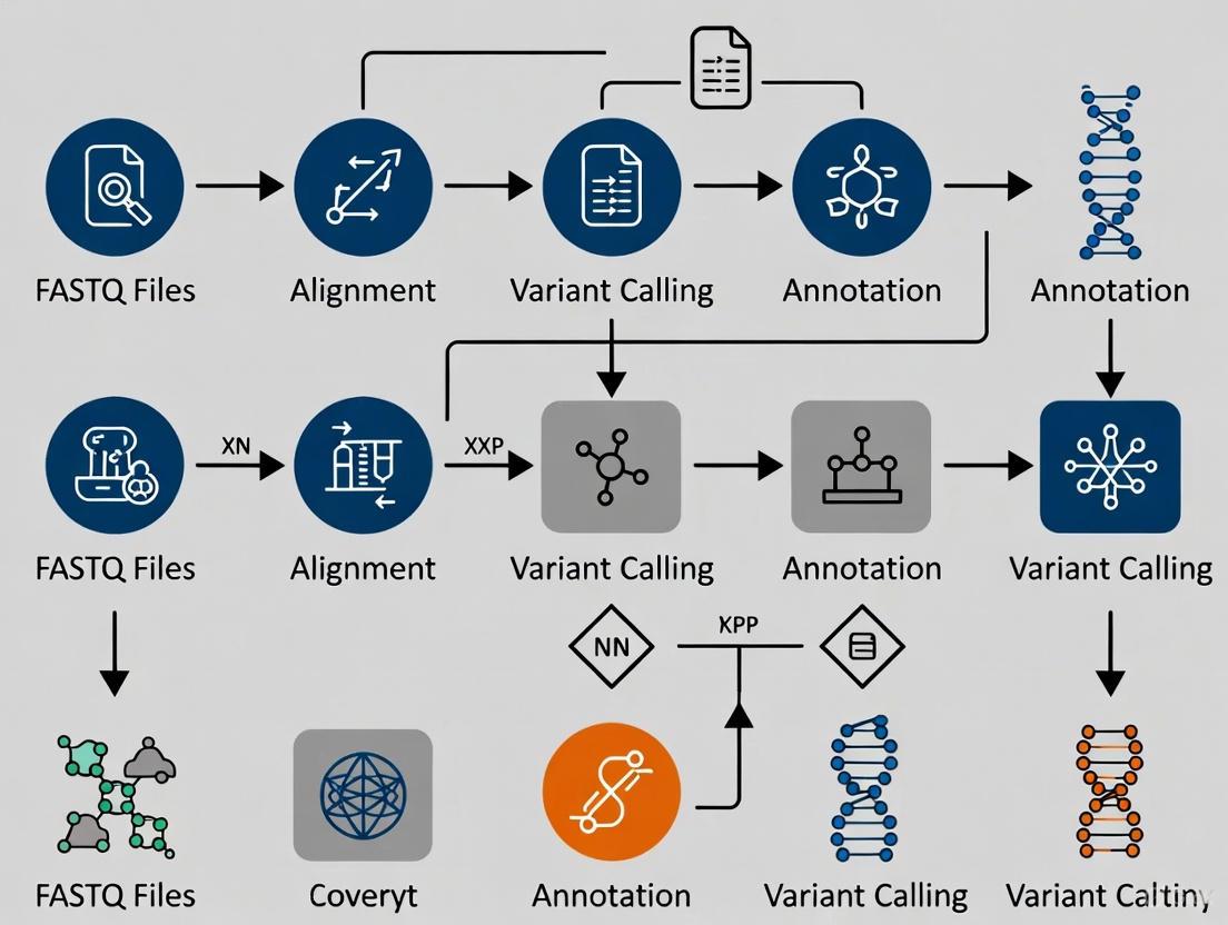
NGS Data Analysis Pipelines for Variant Calling

The raw output of an NGS instrument is a collection of FASTQ files containing millions of short DNA sequences (reads) and their corresponding quality scores. Transforming this data into biologically meaningful variant calls requires a multi-step computational pipeline. The standard reference-based variant calling pipeline involves: 1) Quality Control & Trimming, 2) Read Alignment/Mapping to a reference genome, 3) Post-Alignment Processing (e.g., duplicate marking, base quality recalibration), 4) Variant Calling to identify genomic positions that differ from the reference, and 5) Variant Filtering & Annotation [3].

A significant computational challenge arises from the massive scale of NGS data, especially for large cohorts. This has spurred innovation in distributed computing pipelines. For instance, a 2025 study introduced a scalable, distributed pipeline for reference-free variant calling using a De Bruijn graph constructed from sequencing reads [4]. This approach, implemented with the Apache Spark framework, partitions the graph across multiple machines using a specialized clustering algorithm, enabling efficient parallel processing of large datasets without the bottleneck of aligning all reads to a reference genome first [4].

The most transformative trend in variant calling is the integration of Artificial Intelligence (AI), particularly deep learning (DL). AI-based callers analyze sequencing data in novel ways—for example, by treating aligned reads as multi-channel images—to achieve superior accuracy, especially in complex genomic regions where traditional statistical models struggle [3].

Table: Selected AI-Based Variant Calling Tools (2025)

Tool	Underlying AI Model	Key Feature	Supported Data	Reported Advantage
DeepVariant [3]	Deep Convolutional Neural Network (CNN)	Treats read pileups as images for classification.	Short-read, PacBio HiFi, ONT.	High accuracy, used in large-scale projects like UK Biobank [3].
DeepTrio [3]	Deep CNN (extends DeepVariant)	Jointly analyzes parent-child trios to improve accuracy and identify de novo mutations.	Short-read.	Superior accuracy for family-based studies compared to non-trio methods [3].
DNAscope [3]	Machine Learning (ML) enhancement of core algorithms	Integrates ML-based genotyping with optimized HaplotypeCaller logic.	Short-read, PacBio HiFi, ONT.	High speed and computational efficiency without requiring GPU acceleration [3].
Clair3 [3]	Deep Neural Network	Designed for efficient and accurate calling from both short and long reads.	Short-read, PacBio HiFi, ONT.	Fast performance and good accuracy at lower sequencing coverages [3].

Diagram 2: Standard Reference-Based Variant Calling Pipeline (Max 760px)

Detailed Experimental Protocols

Protocol: Reference-Based Germline SNP/Indel Calling using an AI-Based Pipeline

This protocol outlines the steps for identifying germline single nucleotide polymorphisms (SNPs) and small insertions/deletions (Indels) from whole-genome sequencing data using the DeepVariant pipeline, an accurate AI-based tool [3].

1. Preliminary Setup and Quality Control

• Input: Paired-end FASTQ files (e.g., sample_R1.fastq.gz, sample_R2.fastq.gz).
• Software: Install fastp, samtools, DeepVariant, and associated dependencies. Ensure access to a high-quality reference genome (e.g., GRCh38) and its index.
• Quality Control: Run fastp to perform adapter trimming, quality filtering, and generate QC reports.

2. Read Alignment

• Align trimmed reads to the reference genome using bwa mem. Convert the output SAM file to BAM format, sort it, and index it.

3. Post-Alignment Processing (Optional but Recommended)

• Mark PCR duplicate reads using samtools markdup or Picard Tools. This step is crucial for reducing artifacts in downstream variant calling.

4. Variant Calling with DeepVariant

• Run DeepVariant in its recommended mode. This involves creating labeled examples from the BAM file and running the TensorFlow model to make variant calls.

• The output is a VCF file (sample.deepvariant.vcf.gz) containing unfiltered variant calls with genotype qualities.

5. Variant Filtering and Annotation

• Basic Filtering: While DeepVariant outputs high-quality calls, additional hard-filtering based on quality metrics (e.g., QUAL, DP, GQ) can be applied using bcftools.
• Annotation: Use tools like SnpEff or Ensembl's VEP to annotate variants with functional consequences (e.g., missense, stop-gain), population frequencies, and links to disease databases.

Protocol: Executing a Distributed, Reference-Free Variant Calling Pipeline

This protocol summarizes the method from the 2025 study on scalable, reference-free variant calling for isolated SNPs using a distributed De Bruijn graph on an Apache Spark cluster [4].

1. Input and Environment Setup

• Input: A large collection of raw sequencing reads (FASTQ) from multiple samples.
• Environment: Set up an Apache Spark cluster with multiple worker nodes. Ensure all necessary libraries (e.g., for graph processing) are available.

2. Graph Construction and Partitioning

• k-mer Extraction: The pipeline begins by extracting all k-mers (substrings of length k) from the input reads across all samples in a distributed manner (Map step).
• De Bruijn Graph Assembly: Distinct k-mers are used as vertices. Edges are created between k-mers that overlap by k-1 bases. This constructs a massive, distributed De Bruijn graph representing the collective sequence data.
• Optimized Partitioning: Instead of using Spark's default hash partitioning, the pipeline employs a custom clustering algorithm based on hierarchical clustering and the Jaccard index. This algorithm groups structurally related vertices (i.e., those likely part of the same genomic region) onto the same physical computing node. This minimizes communication overhead between nodes during traversal, which is the key performance innovation [4].

3. Bubble Detection for SNP Identification

• Parallel Graph Traversal: The pipeline traverses the partitioned graph in parallel across all cluster nodes.
• Bubble Recognition: The algorithm searches for specific subgraph patterns called "simple bubbles"—two parallel paths between a common start and end vertex. In a De Bruijn graph, such bubbles often represent alternative alleles at a single genomic locus (i.e., a SNP) [4].
• Variant Output: Each identified bubble is processed to output the candidate isolated SNP, including its sequence context.

4. Performance Consideration

• The study demonstrated that this specialized partitioning strategy led to a relevant performance speed-up compared to standard partitioning techniques, making large-scale reference-free variant calling computationally feasible [4].

The Scientist's Toolkit: Research Reagent Solutions

A successful NGS experiment requires careful selection of reagents and tools at each stage. The following table details key components for a typical variant calling research project.

Table: Essential Research Toolkit for NGS-Based Variant Calling Studies

Category	Item/Reagent	Function & Importance	Example/Note
Library Prep	Fragmentation Enzyme/Kit	Randomly shears DNA to optimal size for sequencing. Critical for library complexity and even coverage.	Acoustic shearing (Covaris) or enzymatic fragmentation (NEB Next Ultra II).
Library Prep	Adapter Ligation Kit	Attaches platform-specific oligonucleotide adapters to DNA fragments. Enables binding to the flow cell and PCR amplification.	Illumina-compatible forked adapters with sample index barcodes for multiplexing.
Library Prep	PCR Enrichment Mix	Amplifies adapter-ligated DNA to create the final sequencing library. Polymerase fidelity impacts error rates.	High-fidelity, low-bias PCR enzymes (e.g., KAPA HiFi).
Sequencing	Sequencing Kit & Flow Cell	Contains enzymes, buffers, and fluorescent nucleotides for the sequencing reaction. The flow cell is the consumable surface where clustering and sequencing occur.	Illumina NovaSeq X Series 25B Reagent Kit, S1/S2 Flow Cell.
Data Analysis	Primary Analysis Software	Performs base calling and demultiplexing on the instrument computer. Converts raw images to FASTQ files.	Illumina DRAGEN, onboard RTA software.
Data Analysis	Variant Calling Pipeline	Core software for identifying genetic variants. Choice depends on required accuracy, speed, and data type.	AI-Based: DeepVariant [3]. Traditional: GATK HaplotypeCaller. Distributed: Custom Apache Spark pipeline [4].
Data Analysis	Variant Annotation Database	Provides biological context (gene, effect, frequency) to raw variant calls. Essential for interpretation.	Local installations of SnpEff/Ensembl VEP with custom databases (gnomAD, ClinVar).
Computational	Workflow Management System	Automates, documents, and ensures reproducibility of multi-step analysis pipelines.	Nextflow, Snakemake [6].
Computational	Containerization Platform	Packages software and dependencies into isolated, portable units to guarantee consistent execution environments.	Docker, Singularity [6].

Economic Impact and Market Trajectory

The widespread adoption of NGS has created a substantial and rapidly growing market for both sequencing services and, critically, the informatics solutions required to analyze the data. The global NGS data analysis market was valued at approximately $5.91 billion in 2025 and is projected to advance at a compound annual growth rate (CAGR) of 16.7%, reaching $14.93 billion by 2033 [7]. Similarly, the broader NGS informatics market is expected to grow from $7.21 billion in 2024 to $25.43 billion by 2035 (CAGR of 12.15%) [8].

This growth is driven by several key factors:

• Expanding Clinical Adoption: NGS is moving from research into routine clinical diagnostics for oncology, rare diseases, and pharmacogenomics [7].
• Government Initiatives: Large-scale national genomics projects (e.g., UK's 100,000 Genomes Project) fuel demand [7].
• Rising Prevalence of Chronic Diseases: Increased focus on cancer and genetic disorders necessitates genomic analysis for personalized treatment strategies [8].
• Technological Advancements: The integration of AI and cloud computing is making analysis faster, more accurate, and more accessible, further propelling market expansion [9].

Geographically, North America currently holds the largest market share due to strong infrastructure and significant investment [8]. However, the Asia-Pacific region is anticipated to be the fastest-growing market, driven by increasing healthcare expenditure, large populations, and rising research funding [8].

The NGS revolution continues to accelerate, with several key trends shaping its future trajectory within variant calling research:

• Convergence of Sequencing Technologies: The distinction between short- and long-read platforms is blurring. Companies are developing multi-omics chemistries (like PacBio's SPRQ for simultaneous sequence and chromatin accessibility detection [5]) and hybrid platforms to offer more comprehensive solutions.
• Ubiquity of AI and Machine Learning: AI will move beyond variant calling to integrate across the entire analysis workflow, including quality control, alignment optimization, and, most importantly, the biological interpretation of variant lists to predict clinical significance [6] [9].
• Democratization and Cloud-Native Analysis: Cloud-based platforms (AWS HealthOmics, Google Cloud Life Sciences) and serverless computing will become the default for many researchers, eliminating local infrastructure barriers and facilitating global collaboration [6]. This must be paired with robust security protocols to protect sensitive genetic data [9].
• Shift to Pangenome References: The use of a single linear reference genome (like GRCh38) will increasingly be supplemented by graph-based pangenome references that incorporate population variation. This will improve alignment accuracy in diverse populations and variant discovery [4] [6].

In conclusion, the journey from Sanger sequencing to high-throughput NGS has unlocked the genomic era. For researchers focused on variant calling, this means navigating a landscape of ever-evolving sequencing technologies, leveraging sophisticated distributed computing pipelines to manage data scale, and employing cutting-edge AI tools to achieve unprecedented accuracy. The future lies in seamlessly integrating these technological advances into robust, reproducible, and accessible analysis workflows. This will fully realize the promise of genomics in driving discoveries in basic biology and delivering on the goals of precision medicine, ultimately transforming how we understand, diagnose, and treat disease.

The translation of raw next-generation sequencing (NGS) data into reliable variant calls constitutes the foundational pillar of modern genomic research and precision medicine. Within the context of a thesis on NGS data analysis pipelines for variant calling, this document establishes that the reproducibility and accuracy of downstream biological insights are inextricably linked to the robustness of the preprocessing and analysis workflow. The transition from FASTQ files, containing raw sequence reads and quality scores, to the final Variant Call Format (VCF) file, is a multi-step computational process where each stage introduces specific biases and errors that can propagate [10]. In clinical and drug development settings, where variants inform diagnoses and therapeutic strategies, non-reproducible results from non-standardized pipelines present a significant challenge [11]. Therefore, a detailed understanding of each essential component—from quality control and alignment to variant calling and filtering—is not merely a technical exercise but a critical scientific requirement for ensuring data integrity, enabling valid cross-study comparisons, and ultimately, supporting confident clinical decision-making [12] [13].

Core Components of the NGS Variant Calling Pipeline

The canonical pipeline for DNA variant discovery follows a logical progression where the output of one stage becomes the input for the next. The following breakdown details the function, key tools, and objectives of each essential component.

1.1. Raw Data & Quality Control (FASTQ) The primary outputs from NGS instruments are FASTQ files, which contain nucleotide sequences for each read and a corresponding per-base quality score (Phred score). The initial Quality Control (QC) step is crucial for identifying issues arising from the sequencing process itself, such as diminishing quality over read length, adapter contamination, or abnormal nucleotide composition. FastQC is the ubiquitous tool for this stage, providing an overview of multiple quality metrics [10]. Findings from QC often necessitate trimming or adapter removal using tools like Trimmomatic or Cutadapt to eliminate low-quality bases or technical sequences before alignment, thereby reducing false mappings and subsequent variant errors [14].

1.2. Read Alignment (BAM/SAM) In this step, cleaned sequence reads are mapped to a reference human genome (e.g., GRCh38). The goal is to determine the genomic origin of each read, accounting for sequencing errors and genuine genetic differences. The Burrows-Wheeler Aligner (BWA-MEM) is a widely adopted, efficient aligner for short reads [12]. The alignment results are stored in Sequence Alignment/Map (SAM) format or its compressed binary version (BAM). SAMtools provides essential utilities for manipulating, sorting, and indexing these files [14]. The integrity and accuracy of the alignment file (BAM) are paramount, as all subsequent variant detection is based on its contents.

1.3. Post-Alignment Processing & Refinement The initial BAM file requires further processing to correct for technical artifacts before variant calling. This stage, often guided by the GATK Best Practices, includes:

• Duplicate Marking: Identification and tagging of PCR duplicate reads (using Picard or SAMtools) that arose from clonal amplification during library preparation, which can bias variant allele frequencies [12].
• Base Quality Score Recalibration (BQSR): A machine-learning technique (GATK BaseRecalibrator) that systematically corrects inaccuracies in the per-base quality scores assigned by the sequencer, using known variant sites (e.g., dbSNP) as a training set [15].
• Local Realignment: Correction of alignment artifacts, particularly around small insertions and deletions (indels), to prevent false-positive variant calls [10]. Following these steps yields an analysis-ready BAM file.

1.4. Variant Calling (VCF) Variant calling algorithms interrogate the processed BAM file to identify genomic positions that differ from the reference. Callers are specialized for different biological contexts and variant types. For germline variants (inherited), GATK HaplotypeCaller is a standard tool that uses a local de novo assembly approach to accurately call SNPs and indels [12]. For somatic variants (acquired, as in cancer), callers compare a tumor sample to a matched normal sample. Mutect2 (part of GATK) and VarScan2 are commonly used somatic callers, each employing different statistical models [16]. The output is a VCF file listing genomic coordinates, reference and alternate alleles, quality scores, and sample-specific genotype information.

1.5. Variant Filtering, Annotation & Interpretation Raw VCF files contain both true biological variants and false positives. Hard filtering (e.g., based on depth, quality, strand bias) or variant quality score recalibration (VQSR) in GATK is applied to refine the call set [12]. Subsequently, annotation tools like SnpEff or VEP add biological context, predicting the functional impact (e.g., missense, stop-gained), population frequency from databases like gnomAD, and links to disease (e.g., ClinVar) [17]. This annotated VCF is the final product for researcher interpretation, visualization in browsers like IGV, and clinical reporting [16].

Table 1: Essential Software Tools for Each Pipeline Stage

Pipeline Stage	Exemplar Tools	Primary Function	Key Output
Quality Control	FastQC [10], Trimmomatic [14]	Assess read quality; remove adapters/low-quality bases.	Trimmed, high-quality FASTQ files.
Read Alignment	BWA-MEM [12], Bowtie2	Map sequencing reads to a reference genome.	Sorted, indexed BAM/SAM file.
Alignment Processing	Picard MarkDuplicates [12], GATK (BQSR, Realigner) [15]	Mark PCR duplicates; recalibrate base qualities; realign indels.	Analysis-ready BAM file.
Variant Calling	Germline: GATK HaplotypeCaller [12], FreeBayes [18]. Somatic: Mutect2 [16], VarScan2 [16], Strelka.	Identify genomic variants relative to the reference.	Raw VCF file.
Variant Refinement	GATK VariantFiltration [12], BCFtools [10]	Filter variants based on quality metrics.	Filtered VCF file.
Annotation	SnpEff [18], VEP [17], ANNOVAR	Add functional, population, and clinical data to variants.	Annotated VCF file.

Detailed Experimental Protocols

2.1. Protocol: Germline Variant Calling via GATK Best Practices Workflow This protocol outlines a standardized pipeline for identifying inherited SNPs and indels from a single sample, using tools compatible with high-performance computing clusters.

• Input: Paired-end FASTQ files (sample_R1.fastq.gz, sample_R2.fastq.gz), human reference genome FASTA (GRCh38.fa) and its pre-built BWA index, known variant sites VCF (dbsnp_146.grch38.vcf).
• Software: BWA (0.7.17), SAMtools (1.9), Picard (2.25.0), GATK (4.2.0).
• Step-by-Step Commands:
  • Map Reads: bwa mem -M -R "@RG\tID:sample\tPL:ILLUMINA\tSM:sample" GRCh38.fa sample_R1.fastq.gz sample_R2.fastq.gz > aligned.sam
  • Sort & Convert to BAM: samtools sort -o sorted.bam aligned.sam then samtools index sorted.bam
  • Mark Duplicates: java -jar picard.jar MarkDuplicates I=sorted.bam O=dedupped.bam M=metrics.txt
  • Base Quality Recalibration: First, build the recalibration model: gatk BaseRecalibrator -I dedupped.bam -R GRCh38.fa --known-sites dbsnp_146.grch38.vcf -O recal_data.table. Then, apply it: gatk ApplyBQSR -I dedupped.bam -R GRCh38.fa --bqsr-recal-file recal_data.table -O recalibrated.bam
  • Variant Calling: gatk HaplotypeCaller -R GRCh38.fa -I recalibrated.bam -O raw_variants.vcf
  • Variant Filtering (SNPs): Apply recommended hard filters: gatk VariantFiltration -R GRCh38.fa -V raw_variants.vcf --filter-expression "QD < 2.0 || FS > 60.0 || MQ < 40.0 || MQRankSum < -12.5 || ReadPosRankSum < -8.0" --filter-name "SNP_FILTER" -O filtered_snps.vcf
• Output: A filtered VCF file (filtered_snps.vcf) containing high-confidence germline variant calls for the sample [12] [15].

2.2. Protocol: Somatic Variant Discovery Using a Three-Caller Consensus Approach To maximize sensitivity and specificity in cancer genomics, a consensus approach combining multiple callers is recommended [16]. This protocol uses matched tumor-normal pairs.

• Input: Analysis-ready BAM files for tumor (tumor.bam) and matched normal (normal.bam), reference genome (GRCh38.fa), panel of normals VCF (PoN), and germline resource (e.g., af-only-gnomad.vcf).
• Software: Mutect2 (GATK 4.2.0), VarScan2 (2.4.3), Strelka2 (2.9.10), BCFtools.
• Step-by-Step Commands:
  • Call variants with Mutect2: gatk Mutect2 -R GRCh38.fa -I tumor.bam -I normal.bam --tumor-sample TUMOR --normal-sample NORMAL --panel-of-normals pon.vcf.gz --germline-resource af-only-gnomad.vcf.gz -O mutect2_unfiltered.vcf
  • Call variants with VarScan2: First, generate an mpileup: samtools mpileup -q 1 -f GRCh38.fa tumor.bam normal.bam > tumor_normal.mpileup. Then run VarScan: varscan somatic tumor_normal.mpileup varscan_output --mpileup 1 --output-vcf 1
  • Call variants with Strelka2: Configure for the BAM files: configureStrelkaSomaticWorkflow.py --tumorBam tumor.bam --normalBam normal.bam --referenceFasta GRCh38.fa --runDir strelka_workflow. Then execute: strelka_workflow/runWorkflow.py -m local -j 8
  • Intersect Callers: Extract PASS variants from each caller's VCF and use bcftools isec to find variants identified by at least two of the three callers: bcftools isec -p output_dir -n +2 mutect2_filtered.vcf varscan_filtered.vcf strelka_snvs.vcf
• Output: A high-confidence somatic VCF file derived from the intersection of multiple callers, significantly reducing false positives while maintaining sensitivity [11] [16].

Quantitative Analysis of Variant Caller Performance

Empirical data underscores the critical impact of tool selection on research outcomes. A study comparing three variant callers on the same 105 breast cancer tumor samples (without matched normal) revealed stark differences in output [11].

Table 2: Comparative Output of Three Variant Callers on 105 Breast Cancer Samples

Variant Caller	Total Variants Called (Aggregate)	Average Variants Per Sample	ClinVar Significant Variants (Aggregate)	Notable Clinical Examples Missed by Other Callers [11]
GATK HaplotypeCaller	25,130	4152.4	1,491	Pathogenic/likely pathogenic variants in ABCA4 (associated with macular degeneration) and CFTR (target of FDA-approved drugs).
VarScan2	16,972	2925.3	1,400	Variants in DHCR7 (linked to Smith-Lemli-Opitz syndrome).
Mutect2 (Tumor-Only Mode)	4,232	159.2	321	Variants in CYP4V2 (associated with Bietti crystalline dystrophy).
Key Finding				An average of 16.5% of clinically significant (ClinVar) variants were detected by only one of the three callers, highlighting the risk of relying on a single algorithm [11].

Integrated Workflow Diagram: From FASTQ to Annotated VCF

NGS Pipeline Main Workflow: FASTQ to VCF

Beyond software, a reliable pipeline requires curated data resources and quality control measures.

Table 3: Key Research Reagent Solutions for Pipeline Implementation

Category	Resource/Reagent	Function & Purpose	Source / Example
Reference Standards	Genome in a Bottle (GIAB) Benchmark Sets [12]	Provides "ground truth" variant calls for reference samples (e.g., NA12878) to validate and benchmark pipeline accuracy.	NIST (National Institute of Standards and Technology)
Reference Data	dbSNP Database [15], gnomAD [15]	Curated databases of known human genetic variants and population frequencies, used for BQSR, filtering, and annotation.	NCBI, Broad Institute
Clinical Annotation	ClinVar Database [11]	Public archive of reports linking human genetic variants to observed health status (pathogenic, benign, etc.).	NCBI
Quality Control	Picard Metrics (HsMetrics, AlignmentSummary) [13]	Suite of tools to generate quantitative metrics (e.g., coverage uniformity, insert size) for verifying library prep and sequencing quality.	Broad Institute
Validation	Synthetic Diploid (Syndip) Benchmark [12]	A less biased benchmarking dataset derived from long-read assemblies, useful for evaluating performance in complex genomic regions.	Available via sequencing repositories
Containerization	Docker/Singularity Containers	Packages the entire pipeline software environment to guarantee absolute reproducibility and portability across computing platforms.	Container registries (Docker Hub, Biocontainers)

The advent of Next-Generation Sequencing (NGS) has revolutionized genomics, enabling the rapid, high-throughput analysis of DNA and RNA to drive progress in cancer research, rare disease diagnosis, and personalized medicine [19]. The transformation of raw sequencing signals into actionable biological insights hinges on a robust and reproducible bioinformatics pipeline. This pipeline is universally structured around three critical, sequential data processing steps: Quality Control (QC), Alignment (Mapping), and Variant Calling [19]. The integrity of each step is paramount, as errors introduced early in the workflow propagate and magnify, potentially leading to false conclusions in downstream analyses. This thesis frames these technical steps within the broader context of constructing reliable NGS analysis pipelines for variant discovery research, emphasizing standardized protocols, performance metrics, and the emerging integration of artificial intelligence (AI) to enhance accuracy and scalability [20] [3].

Primary Analysis and Data Quality Control

Primary Analysis constitutes the first computational assessment of raw sequencing data, typically performed by the instrument's software or dedicated pipelines like bcl2fastq. This step translates raw signal data (e.g., .bcl files from Illumina platforms) into nucleotide sequences, generating FASTQ files that contain read sequences and their corresponding per-base quality scores [21]. Quality Control (QC) is an inseparable and iterative component of primary and secondary analysis, designed to evaluate data integrity and filter technical artifacts before biological interpretation.

Key Quality Metrics and Assessment Protocols

Rigorous QC employs both quantitative metrics and visual assessments. The cornerstone metric is the Phred Quality Score (Q-score), which is logarithmically linked to base-calling error probability (Q20 = 99% accuracy, Q30 = 99.9% accuracy). A Q-score ≥ 30 across the majority of bases is a standard benchmark for high-quality data [21].

Table 1: Core Quality Control Metrics for NGS Data [21] [22]

Metric	Description	Optimal Range / Target
Per-base Sequence Quality	Phred score distribution across all sequencing cycles.	Q ≥ 30 for majority of bases.
Per-sequence Quality	Average quality score for each read.	High mean score; few outliers.
Sequence Length Distribution	Distribution of read lengths after trimming.	Uniform, as expected from library prep.
Adapter Contamination	Presence of adapter sequences in reads.	Minimal to none after trimming.
GC Content	Distribution of guanine-cytosine content per read.	Matches reference organism's distribution.
Sequence Duplication Level	Proportion of PCR/optical duplicates.	Low percentage; context-dependent.
Overrepresented Sequences	Sequences appearing at high frequency.	Investigate sources (e.g., contaminants).

A standard QC protocol involves using tools like FastQC for initial assessment and Trimmomatic or Cutadapt for read cleaning [23]. The workflow is: 1) Run FastQC on raw FASTQ files; 2) Trim adapter sequences and low-quality bases from read ends (e.g., using a sliding window trimming approach); 3) Remove reads falling below a minimum length threshold (e.g., < 36 bp); 4) Run FastQC again on the trimmed files to verify improvement [23] [21]. For advanced applications, Unique Molecular Identifiers (UMIs) are used during library preparation to enable accurate deduplication at the level of original molecules, correcting for PCR amplification bias [21].

Visualizing the Quality Control Workflow

The following diagram illustrates the iterative and branching nature of a standard QC workflow, from raw data to cleaned reads ready for alignment.

Diagram: Iterative NGS Data Quality Control and Cleaning Workflow

Sequence Alignment to a Reference Genome

Alignment (or mapping) is the process of determining the genomic origin of each sequencing read by computationally matching it to a location within a reference genome. The accuracy of alignment directly influences the sensitivity and precision of all subsequent variant detection [19].

Alignment Algorithms and Tools

Alignment tools must efficiently handle millions of short reads against a gigabase-sized reference. Most aligners, such as the widely adopted Burrows-Wheeler Aligner (BWA) and Bowtie2, use a seed-and-extend strategy with sophisticated indexing (e.g., FM-index) for speed [23] [21]. The choice of reference genome is critical; for human studies, the current standard is GRCh38/hg38, though GRCh37/hg19 remains in widespread use [24] [21]. Consistency in the reference version across an entire study is essential.

The alignment protocol involves two main steps [23]:

• Indexing the Reference Genome (one-time operation):

• Mapping Reads (per sample):

The output is a Sequence Alignment/Map (SAM) file, a tab-delimited text file detailing each read's mapping position, alignment quality (MAPQ score), and CIGAR string representing matches, insertions, deletions, and splices [23]. SAMtools is then used to convert the SAM file to its compressed binary equivalent, the BAM file, sort it by genomic coordinate, and index it for rapid access [23]:

Post-Alignment Processing and Visualization

The sorted BAM file undergoes further refinement before variant calling [24]:

• Duplicate Marking/Removal: Identifies and flags reads originating from the same PCR amplicon or optical duplicate using tools like Picard MarkDuplicates to prevent bias in variant allele frequency calculations.
• Local Realignment: Tools like the GATK HaplotypeCaller perform local realignment around indels to correct mapping artifacts.
• Base Quality Score Recalibration (BQSR): Uses known variant sites to empirically adjust base quality scores, correcting for systematic technical errors.

Alignment success is evaluated using metrics like mapping rate (percentage of reads mapped), depth of coverage (average reads covering a base), and coverage uniformity [21]. Visualization with genome browsers like the Integrative Genomics Viewer (IGV) is crucial for manual inspection of read pileups, splice junctions, and potential variant sites [24] [21].

Table 2: Common Alignment and Post-Processing Tools

Tool	Primary Function	Key Notes
BWA (MEM)	Short-read alignment.	Industry standard for speed/accuracy balance [23] [21].
Bowtie2	Short-read alignment.	Fast, especially for shorter reads [21].
Minimap2	Long-read/pacBio/Nanopore alignment.	Standard for aligning long-read sequencing data.
SAMtools	Manipulate/view SAM/BAM files.	Essential utility for sorting, indexing, and filtering [23].
Picard	Java-based tools for BAM processing.	Standard for duplicate marking and metric collection.
GATK	Broad toolkit for variant discovery.	Provides Best Practices pipelines for realignment, BQSR, and calling [24].
IGV	Interactive visualization.	Critical for inspecting alignments and validating calls [24] [21].

Variant Calling: From Aligned Reads to Genetic Variants

Variant calling is the comparative analysis of aligned reads against a reference genome to identify sites of genetic difference. These variants include Single Nucleotide Polymorphisms (SNPs), small Insertions/Deletions (Indels), and larger Structural Variations (SVs) [24].

Methodologies: From Traditional Heuristics to AI

Traditional variant callers (e.g., GATK HaplotypeCaller, SAMtools mpileup) use statistical models and heuristic rules. For example, the HaplotypeCaller works by: 1) Identifying active regions; 2) Assembling reads into potential haplotypes; 3) Determining likelihoods of haplotypes given the read data; 4) Assigning sample genotypes [24]. The output is a Variant Call Format (VCF) file, which records the genomic position, reference/alternate alleles, quality scores, and sample genotype information for each variant [24] [23].

A paradigm shift is underway with the adoption of AI-based variant callers, which use deep learning models (typically Convolutional Neural Networks - CNNs) trained on vast datasets to distinguish true variants from sequencing artifacts [20] [3].

Table 3: Comparison of AI-Enhanced Variant Callers [3]

Caller	Core Technology	Key Strength	Consideration
DeepVariant	CNN analyzing read pileup images.	Exceptional accuracy; reduces need for hard filtering.	High computational cost (GPU recommended).
DNAscope	Machine learning-enhanced algorithm.	High speed and accuracy; efficient CPU-based.	ML-based, not a deep learning model per se.
DeepTrio	CNN for family trio analysis.	Jointly calls families, improving de novo mutation detection.	Requires trio data.
Clair/Clair3	CNN optimized for long-read data.	High performance for PacBio HiFi and Nanopore.	Actively developed for long-read tech.

A protocol for traditional germline variant calling with bcftools involves [23]:

For AI-based calling with DeepVariant, the protocol shifts to using a pre-trained model:

Variant Filtering, Annotation, and the Integrated Workflow

Raw variant calls contain false positives. Filtering applies thresholds on metrics like QUAL (phred-scaled probability of variant), DP (read depth), and QD (quality by depth) to refine the call set [24]. Variant annotation using tools like SnpEff or ANNOVAR adds biological context, predicting the effect on genes (e.g., missense, frameshift), and overlaying population frequency data from databases like dbSNP, gnomAD, and COSMIC [24] [19].

The complete logical relationship from raw data to annotated variants is summarized in the following sequential workflow diagram.

Diagram: Core NGS Variant Calling Pipeline with AI Integration Points

Constructing and executing a reliable NGS analysis pipeline requires both software tools and curated data resources. The following toolkit is essential for researchers in variant calling.

Table 4: Essential Research Reagent Solutions for NGS Variant Analysis

Category	Item / Resource	Function / Purpose	Example / Source
Wet-Lab Preparation	Library Prep Kits	Fragment DNA/RNA, add adapters & indices for sequencing.	Illumina TruSeq, NEBNext.
Wet-Lab Preparation	Unique Molecular Identifiers (UMIs)	Tag individual molecules pre-PCR to correct for duplication bias.	Integrated UMI adapters.
Wet-Lab Preparation	Positive Control DNA	Assess sequencing run performance and error rates.	PhiX Control v3 (Illumina).
Computational Tools	QC & Trimming Software	Assess raw data quality and remove artifacts.	FastQC [22], Trimmomatic [23].
Computational Tools	Alignment Software	Map sequencing reads to a reference genome.	BWA [23] [21], Bowtie2 [21].
Computational Tools	Variant Callers	Identify genetic variants from aligned reads.	GATK [24], DeepVariant [3], DNAscope [3].
Computational Tools	VCF Manipulation	Filter, compare, and manipulate variant files.	BCFtools [23], SnpSift [24], VCFtools.
Computational Tools	Visualization Software	Manually inspect alignments and variant calls.	IGV [24] [21], Tablet.
Reference Data	Reference Genomes	Standardized genomic sequence for alignment.	GRCh38 from Genome Reference Consortium [24].
Reference Data	Variant Databases	Annotate variants with known frequency/pathogenicity.	dbSNP [19], gnomAD, ClinVar [24], COSMIC [19].
Reference Data	Gene Annotation	Define genomic coordinates of genes and transcripts.	GENCODE, RefSeq.
Infrastructure	High-Performance Compute	Process large NGS datasets in a reasonable time.	Local cluster (HPC) or cloud (AWS, GCP, Azure).
Infrastructure	Workflow Managers	Automate, reproduce, and scale analysis pipelines.	Nextflow, Snakemake, WDL/Cromwell.

The triad of Quality Control, Alignment, and Variant Calling forms the foundational, non-negotiable core of any NGS analysis pipeline for variant research. As sequencing technologies evolve toward long-read and single-cell applications, and data volumes grow, these steps must adapt [2]. The integration of Artificial Intelligence is the most transformative current trend, with AI models demonstrating superior accuracy in basecalling, alignment optimization, and particularly in variant calling, where they reduce false positives in challenging genomic regions [20] [3]. Future pipelines will increasingly be AI-native, leveraging federated learning for privacy-preserving analysis on distributed datasets and explainable AI (XAI) to build clinical trust [20]. For researchers and drug development professionals, mastery of both the established principles outlined here and the emerging AI-enhanced methodologies is critical to generating the high-fidelity genomic insights that underpin modern precision medicine [19].

The comprehensive identification and interpretation of genomic variation form the cornerstone of advanced genetic research, clinical diagnostics, and therapeutic development. Within the framework of Next-Generation Sequencing (NGS) data analysis pipelines, variant calling is the critical process that translates raw sequencing data into a catalog of DNA sequence differences relative to a reference genome [4]. These variants are traditionally classified by size and complexity into several major types: Single Nucleotide Variants (SNVs), short Insertions and Deletions (Indels), Copy Number Variants (CNVs), and broader Structural Variations (SVs) [25]. Each category presents unique challenges for detection and requires specialized computational approaches, especially when comparing the capabilities of prevalent short-read sequencing with emerging long-read technologies [25]. The accurate delineation of this full spectrum of variation is essential for unraveling the genetic basis of diseases, from Mendelian disorders to complex neurodevelopmental conditions like autism spectrum disorder (ASD), where a significant diagnostic gap remains despite high heritability [26]. This article provides detailed application notes and protocols for detecting these variant types, framed within the context of building robust NGS data analysis pipelines for research and clinical applications.

Defining the Variant Landscape

Genomic variants are systematically categorized based on their molecular characteristics and size, which directly influence the choice of sequencing technology and computational tool required for their discovery.

Table 1: Classification and Characteristics of Major Variant Types

Variant Type	Size Range	Description	Common Subtypes	Detection Challenge
Single Nucleotide Variant (SNV)	1 bp	A substitution of one single nucleotide for another.	Transition (AG, CT), Transversion (all other swaps).	Distinguishing true variants from sequencing errors; genotyping in low-complexity regions.
Insertion/Deletion (Indel)	< 50 bp	The insertion or deletion of a small number of nucleotides.	Insertion, Deletion.	Accurate alignment of reads around the variant; size bias in short-read data (insertions >10 bp are poorly detected) [25].
Copy Number Variant (CNV)	> 50 bp	A large-scale deletion or duplication of a genomic segment, altering the copy number.	Deletion (CN loss), Duplication (CN gain).	Differentiating from technical read-depth fluctuations; precise breakpoint resolution.
Structural Variation (SV)	≥ 50 bp	Genomic rearrangements that may or may not alter copy number.	Deletion, Duplication, Insertion, Inversion, Translocation, Complex Rearrangement [26].	Detection in repetitive genomic regions (e.g., segmental duplications) is difficult with short reads [25].

CNVs are often considered a subset of SVs focused specifically on copy-number changes. The >50 bp threshold distinguishing indels from SVs is conventional, but the detection limit for short-read-based indel callers is often lower, around 10-15% of the read length [25]. Long-read sequencing (e.g., PacBio HiFi, Oxford Nanopore) is particularly powerful for resolving SVs and larger indels because its reads span complex and repetitive regions [25] [26].

Variant Detection within NGS Analysis Pipelines

A generic, high-level workflow for germline variant calling from whole-genome sequencing (WGS) data involves sequential steps from raw data to annotated variants. This pipeline must be adapted based on the sequencing technology (short- vs. long-read) and the variant type of interest.

High-Level NGS Variant Calling Pipeline Workflow

Pipeline Architecture Considerations: Modern pipelines must integrate both reference-based and emerging reference-free or alignment-free (AF) approaches. Reference-based methods align reads to a linear reference genome (e.g., GRCh38) and look for discrepancies [4]. In contrast, reference-free methods, such as those based on De Bruijn graphs, construct sequence relationships directly from reads to identify polymorphisms like isolated SNPs without alignment, which can be advantageous for non-model organisms or highly polymorphic regions [4]. Scalability is a critical concern, leading to the development of distributed pipelines using frameworks like Apache Spark to parallelize tasks such as graph construction and k-mer counting across compute clusters, making the analysis of large cohorts feasible [4].

Detailed Experimental Protocols

Protocol: Germline SNV and Indel Calling from Short-Read WGS

This protocol is validated for human whole-genome sequencing data from Illumina or DNBSEQ platforms (coverage >30x) aligned to GRCh37/38 [25] [27].

Materials:

• Input: Paired-end FASTQ files.
• Software: FastQC, Trimmomatic, BWA-MEM, SAMtools, GATK (v4.0+), DeepVariant.
• Reference Files: Reference genome (FASTA), known variant sites (dbSNP, gnomAD).

Procedure:

• Quality Control: Assess raw reads with FastQC. Trim adapters and low-quality bases using Trimmomatic.
• Alignment: Align reads to the reference genome using BWA-MEM. Convert SAM to sorted BAM with SAMtools.
• Post-Alignment Processing: Mark duplicate reads with GATK MarkDuplicates. Perform base quality score recalibration (BQSR) using GATK BaseRecalibrator and known variant sites.
• Variant Calling: Call SNVs and small indels using a primary caller (e.g., GATK HaplotypeCaller in GVCF mode). For enhanced accuracy, especially in difficult regions, consider a deep learning-based caller like DeepVariant [25].
• Joint Genotyping & Filtering: If processing a cohort, perform joint genotyping on all samples' GVCFs using GATK GenotypeGVCFs. Apply variant quality score recalibration (VQSR) or hard filters (e.g., GATK VariantFiltration) to remove low-confidence calls.
• Annotation: Annotate the final VCF file with functional consequences using SnpEff or Ensembl VEP.

Protocol: Structural Variant Detection from Long-Read WGS

This protocol is designed for detecting SVs (≥50 bp) using Oxford Nanopore or PacBio HiFi data, as applied in studies of neurodevelopmental disorders [26].

Materials:

• Input: High molecular weight (HMW) genomic DNA (>20 kb fragment size), Oxford Nanopore SQK-LSK114 ligation kit, R10.4.1 flow cells [26].
• Software: Guppy (basecalling), Minimap2, Samtools, cuteSV, Sniffles2, SVIM, AnnotSV.

Procedure:

• Library Preparation & Sequencing: Prepare an amplification-free library from 1 µg of HMW gDNA using the ligation sequencing kit per manufacturer instructions [26]. Load onto a MinION Mk1C sequencer for ~48 hours to achieve a target coverage of >7x per run [26].
• Basecalling & Alignment: Perform high-accuracy basecalling on raw FAST5/POD5 files using Guppy (super-accurate model). Align the resulting FASTQ files to the GRCh38 reference genome using Minimap2 with the -ax map-ont preset.
• SV Calling & Consolidation: Call SVs using multiple callers for robustness (e.g., cuteSV, Sniffles2, SVIM) [26]. To generate a high-confidence set, select SVs detected by at least 3 out of 5 callers, requiring breakpoint proximity (≤200 bp for insertions) or reciprocal overlap (≥50% for others) [25] [26].
• Annotation & Prioritization: Annotate the high-confidence SV set with AnnotSV to identify overlaps with genes, regulatory elements, and known pathogenic regions. Prioritize rare, genic, or copy-number altering SVs for further validation.

Performance Comparison of Technologies and Tools

The choice of sequencing platform and analytical tool significantly impacts the sensitivity and precision of variant detection, particularly for indels and SVs.

Table 2: Performance of Short-Read vs. Long-Read Sequencing for Variant Detection [25]

Variant Type	Key Metric	Short-Read Performance	Long-Read Performance	Contextual Note
SNV	Recall & Precision	High	High	Comparable performance in non-repetitive regions [25].
Indel (Deletion)	Recall & Precision	High	High	Comparable performance [25].
Indel (Insertion >10bp)	Recall	Low (Poorly detected)	High	Short-read algorithms struggle with insertions >10 bp [25].
SV (All)	Recall in Repetitive Regions	Significantly Lower	Higher	Short-read recall is low for small-to-intermediate SVs in repeats [25].
SV (All)	Recall/Precision in Non-Repetitive	Moderate	Moderate	Similar performance between technologies in accessible regions [25].

Table 3: Detection Metrics for SVs Across Sequencing Platforms (NA12878 Sample) [28]

SV Type	Platform	Average Number Detected	Average Precision	Average Sensitivity
Deletion (DEL)	Illumina	2,676	53.06%	9.81%
Deletion (DEL)	DNBSEQ	2,838	62.19%	15.67%
Insertion (INS)	Illumina	737	44.01%	2.80%
Insertion (INS)	DNBSEQ	1,117	43.98%	3.17%
Inversion (INV)	Illumina	239	26.79%	11.06%
Inversion (INV)	DNBSEQ	422	25.22%	11.58%

Data shows high consistency between DNBSEQ and Illumina platforms for SV detection, with DNBSEQ showing marginally higher sensitivity for deletions [28]. Overall, sensitivity for INS and INV remains low with short-read technologies, underscoring a limitation.

The algorithmic approach of the variant caller is paramount. SV detection tools for short-read data rely on indirect signals like read depth (RD), split reads (SR), read pairs (RP), or a combination (CA) [28]. Each has strengths and weaknesses, leading to the recommendation of using multiple callers and integrating their results.

Short-Read SV Detection Algorithms and Their Targets

The Scientist's Toolkit: Essential Reagents and Software

Table 4: Key Research Reagent Solutions for Variant Discovery

Item Name	Category	Function in Workflow	Example/Supplier
High Molecular Weight gDNA Kit	Sample Prep	Extracts long, intact genomic DNA essential for long-read sequencing and reliable SV detection.	Qiagen Genomic-tip, Nanobind CBB.
PCR-Free Library Prep Kit	Library Prep	Prevents amplification bias, improving uniform coverage and accurate detection of SNVs, indels, and CNVs [27].	Illumina DNA PCR-Free Prep, Tagmentation [27].
Ligation Sequencing Kit	Library Prep (Long-Read)	Prepares amplification-free libraries for Oxford Nanopore sequencing, preserving native DNA for long reads.	Oxford Nanopore SQK-LSK114 [26].
BWA-MEM2	Alignment Software	Aligns short sequencing reads to a reference genome quickly and accurately.	Open-source aligner.
Minimap2	Alignment Software	Aligns long, error-prone reads (ONT/PacBio) to a reference genome.	Open-source aligner [25].
GATK HaplotypeCaller	Variant Caller	The industry standard for calling germline SNVs and indels from short-read data.	Broad Institute.
DeepVariant	Variant Caller	Uses a deep learning model to call SNVs and indels from aligned reads, often outperforming traditional methods [25].	Google Health.
cuteSV / Sniffles2	Variant Caller	Specialized tools for sensitive detection of SVs from long-read sequencing data [26].	Open-source.
AnnotSV	Annotation Tool	Comprehensively annotates structural variants with gene, regulatory, and disease association information.	Open-source [26].

A comprehensive understanding of SNVs, Indels, CNVs, and SVs is fundamental to exploiting NGS data fully. As evidenced, no single technology or tool captures the complete variome. Short-read sequencing excels in cost-effective, accurate SNV and small indel detection, while long-read sequencing is indispensable for resolving complex SVs and large insertions, particularly in repetitive regions [25] [26]. The future of variant calling pipelines lies in integrative approaches: combining short- and long-read data (hybrid sequencing), leveraging ensemble calling methods across multiple algorithms, and incorporating population-scale resources and pangenome graphs to reduce reference bias [4]. For clinical translation, as demonstrated by lab-developed procedures (LDPs) for population screening, rigorous validation of wet-lab and computational components is essential to achieve the high sensitivity and specificity required for reporting actionable findings in genes associated with hereditary disease and pharmacogenomics [27]. By strategically selecting and combining the protocols and tools outlined here, researchers can construct robust analysis pipelines to unlock the full spectrum of genomic variation.

Reference Genomes and Their Impact on Variant Discovery

Within the framework of next-generation sequencing (NGS) data analysis pipelines for variant calling research, the choice of reference genome is a foundational determinant of accuracy and comprehensiveness. A reference genome serves as the standard coordinate system against which sample reads are aligned to identify genetic differences. The evolution from single, linear references to more sophisticated graph-based and population-aware genomes directly addresses historical limitations, enabling more precise variant discovery in complex genomic regions [29]. This progression is critical for applications in clinical genomics, drug target discovery, and personalized medicine, where missing or mis-calling a variant can alter biological interpretation and downstream clinical decisions [2] [30].

The central challenge in variant discovery is distinguishing true biological variants from sequencing artifacts and alignment errors. This challenge is most acute in difficult-to-map regions such as segmental duplications, low-complexity repeats, and highly polymorphic loci like the Major Histocompatibility Complex (MHC) [31] [29]. Traditional linear references, representing a mosaic of haplotypes from a few individuals, provide a poor representation of global genetic diversity. Consequently, reads from an individual that diverge from the reference in these complex regions may map poorly or incorrectly, leading to false negatives (missing real variants) or false positives (artifactual calls) [31]. Advancements in reference genomes are therefore not merely incremental improvements but essential refinements that enhance the fidelity of the entire NGS analysis pipeline.

Evolution and Types of Reference Genomes

The landscape of human reference genomes has progressed significantly, moving beyond a single canonical sequence to incorporate population diversity and alternate genomic pathways. This evolution is summarized in the diagram below.

Linear Reference Genomes and Their Limitations

The widely used GRCh37/hg19 and GRCh38/hg38 assemblies from the Genome Reference Consortium are linear, monolithic sequences [29]. GRCh38 introduced significant improvements, including corrected misassemblies and expanded coverage of complex regions. A key feature of the official GRCh38 assembly is the inclusion of alternative (ALT) contigs—long, alternative haplotype sequences for approximately 60 genomic loci, providing alternate representations for highly variable regions [29]. However, a major limitation is that these ALT contigs are assembled from a very small number of individuals and are not fully integrated into the primary chromosome sequences, complicating their use during read alignment.

To mitigate mapping ambiguity, enhanced versions of the linear reference incorporate decoy sequences (often derived from alternative haplotypes and common microbial contaminants) that "catch" reads that would otherwise map ambiguously to multiple primary locations. Furthermore, the approach to handling native ALT contigs has evolved. The initial "ALT-aware" method used complex liftover alignments but could create dense clusters of mismapped reads [29]. The newer, recommended ALT-masking strategy strategically masks ALT contig segments that are highly similar to the primary assembly, preventing them from competitively stealing alignments. Divergent segments remain unmasked, functioning as decoys. This approach simplifies the analysis and improves variant calling accuracy over the liftover-based method [29].

Graph-based references represent a paradigm shift by explicitly incorporating known genetic variation (e.g., from the 1000 Genomes Project) directly into the reference structure [31] [29]. Instead of one linear path, the reference is a graph with nodes (sequence blocks) and edges (connections). Common haplotypes form alternate paths through the graph. During alignment, a read that differs from the primary path but matches a known alternate haplotype path can map with higher confidence and quality. This is particularly powerful for resolving reads in difficult, polymorphic regions where a linear reference provides a poor match [29]. Tools like Illumina's DRAGEN employ such graph genomes, which have been shown to improve accuracy in benchmark challenges [29].

The Emerging Pangenome

The most comprehensive evolution is the concept of a human pangenome, which aims to represent the full spectrum of human genetic diversity by assembling complete genomes from hundreds of diverse individuals [31]. This collective reference moves beyond a single coordinate system to a truly population-aware framework, promising to dramatically reduce reference bias and improve variant discovery equity across all ancestries.

Table 1: Comparison of Major Human Reference Genome Types

Reference Type	Key Characteristics	Primary Advantage	Key Limitation	Example/Version
Canonical Linear	Single, monolithic sequence for each chromosome.	Simplicity; standard for annotation and reporting.	High reference bias; poor representation of diversity.	GRCh37, GRCh38 primary assembly [29].
Enhanced Linear (with ALT/Decoy)	Primary assembly supplemented with alternative contigs and decoy sequences.	Reduces ambiguous mapping for reads similar to paralogous regions.	ALT contigs are discrete, unphased, and from limited haplotypes [29].	GRCh38 full assembly (with ALT), hg38 with decoys.
ALT-Masked	Enhanced linear reference where problematic segments of ALT contigs are masked.	Prevents mapping artifacts from incorrect ALT liftover, improving accuracy [29].	Still based on a limited set of alternate haplotypes.	DRAGEN hg38-alt-masked reference [29].
Graph-Based	Encodes population haplotypes as alternate paths within a graph data structure.	Dramatically improves mapping accuracy and variant calling in polymorphic and difficult regions [31] [29].	Computational complexity; larger reference size.	DRAGEN hg38 graph reference [29].
Pangenome	Collection of multiple, complete genome assemblies from diverse individuals.	Minimizes reference bias; represents global genetic diversity.	In early stages of development and adoption; complex to use.	Human Pangenome Reference Consortium assemblies [31].

Quantitative Impact on Variant Calling Accuracy

The choice of reference genome has a measurable, direct impact on key performance metrics in variant calling: precision (the fraction of calls that are real) and recall (the fraction of real variants that are called).

Impact on Small Variant Calling

Benchmarking using gold-standard datasets like those from the Genome in a Bottle (GIAB) consortium quantifies this impact. For small variants (SNVs and indels), using an ALT-masked reference reduces false positives and false negatives compared to older ALT-aware methods. Furthermore, transitioning from a standard linear reference to a graph-based reference yields significant gains. For example, in the GIAB benchmark, using a DRAGEN graph reference showed improved accuracy for both SNPs and indels compared to its non-graph counterpart [29]. A 2025 benchmarking study of whole-exome sequencing software found that the highest-performing pipeline (DRAGEN Enrichment) achieved precision and recall scores >99% for SNVs and >96% for indels against GIAB truth sets, a benchmark that assumes the use of an optimized reference [32].

Impact on Structural Variant (SV) Calling

The effect is even more pronounced for structural variants (SVs), which are often rooted in complex, repetitive, or duplicated sequences. Studies demonstrate that leveraging a graph-based multigenome reference significantly improves SV calling in complex genomic regions compared to the standard linear GRCh38 [31]. This is because graph references provide the necessary context to correctly place reads spanning breakpoints or within segmental duplications. The performance gap between short-read (srWGS) and long-read sequencing (lrWGS) for SV detection also narrows with better references, as improved mapping in difficult regions boosts the sensitivity of srWGS [31].

Table 2: Performance Metrics of Leading Variant Callers (2025 Benchmark)

Variant Calling Software / Pipeline	SNV Precision (%)	SNV Recall (%)	Indel Precision (%)	Indel Recall (%)	Average Runtime (WES Sample)	Reference Genome Used
Illumina DRAGEN Enrichment	>99	>99	>96	>96	29-36 minutes [32]	GRCh38 (graph-based assumed)
CLC Genomics Workbench	>98	>98	~94	~94	6-25 minutes [32]	GRCh38
Varsome Clinical	>98	>98	~93	~94	Not Specified	GRCh38
Partek Flow (GATK)	>98	>98	~92	~92	3.6 - 29.7 hours [32]	GRCh38
GATK Best Practices (BWA + GATK)	High (Literature)	High (Literature)	High (Literature)	High (Literature)	Hours (Cluster-dependent)	GRCh38 (typically)

Experimental Protocols for Benchmarking Reference Genome Performance

To empirically evaluate the impact of different reference genomes on a variant calling pipeline, researchers should conduct systematic benchmarking. The following protocol outlines a robust methodology based on current best practices [31] [32].

Protocol: Benchmarking Reference Genome Impact on SV Calling

Objective: To assess the precision and recall of structural variant (deletion) calling using short-read data aligned to different versions of the GRCh38 reference genome.

Materials:

• Benchmark Sample: HG002 (Ashkenazim son) sequencing data (Illumina WGS, 25-30x coverage). Download from GIAB FTP site [31].
• Truth Set: GIAB HG002 Tier 1 deletion callset (v0.6, lifted to GRCh38) [31].
• Reference Genomes:
  • GRCh38 primary assembly only.
  • GRCh38 with decoy sequences (e.g., hg38.fa with hs38d1 decoy).
  • GRCh38 ALT-masked reference (e.g., DRAGEN hg38-alt-masked) [29].
  • GRCH38 graph-based reference (e.g., DRAGEN hg38-alt-masked-graph) [29].
• Software: DRAGEN Bio-IT Platform (v4.2 or higher) or open-source aligner (minimap2, DRAGMAP) + SV caller (Manta, DRAGEN SV caller). BEDTools for region analysis.

Procedure:

• Data Preparation: Subsample HG002 FASTQ files to a uniform coverage (e.g., 30x) using seqtk.
• Alignment & Calling (Parallel Runs): For each reference genome (Ref1-4): a. Align reads using the dragen command with the --ht-reference pointing to the reference hash table, or use minimap2 -ax sr. b. Perform SV calling focused on deletions. In DRAGEN, use the SV Calling Workflow. With Manta, configure and run runMantaWorkflow.py. c. Filter output VCF to PASS variants and variant type DEL.
• Benchmarking: Compare each resulting VCF against the GIAB Tier 1 truth set using hap.py (vcfeval) or truvari. a. Use the high-confidence region BED file from GIAB to restrict evaluation. b. Calculate precision = TP/(TP+FP) and recall = TP/(TP+FN).
• Region-Specific Analysis: Stratify performance in Low-Complexity Regions (LCRs). Use a BED file defining LCRs to intersect the variant calls and truth set, then recalculate metrics for variants inside and outside these regions [31].

Expected Outcome: A clear gradient of improving recall (and often precision) is expected, moving from the primary assembly to the graph-based reference, with the most significant improvements observed within LCRs and other difficult-to-map regions [31] [29].

Protocol: Evaluating Reference Impact on Small Variant Calling in Exomes

Objective: To measure the effect of reference choice on SNV and indel detection accuracy in whole-exome sequencing data.

Materials:

• Benchmark Samples: GIAB WES data for HG001, HG002, and HG003 (Agilent SureSelect V5) [32].
• Truth Sets: GIAB small variant truth sets (v4.2.1) for each sample.
• Reference Genomes: GRCh38 standard vs. GRCh38 graph-based.
• Software: DRAGEN Enrichment pipeline or GATK Best Practices pipeline (BWA-MEM + GATK HaplotypeCaller), hap.py for benchmarking.

Procedure:

• Pipeline Execution: Process each sample's FASTQs through the chosen variant calling pipeline twice—once with the standard linear GRCh38 and once with the graph-based GRCh38 reference. Keep all other parameters identical.
• Variant Evaluation: Run hap.py on the two output VCFs for each sample against their respective truth sets, confined to the exome capture regions.
• Metrics Collection: Record the F1 score (harmonic mean of precision and recall), stratified by variant type (SNV, insertion, deletion) and genomic context (e.g., high-confidence regions vs. all targeted bases).
• Variant Concordance Analysis: Use bcftools isec to identify variants unique to each reference run. Manually inspect a subset of discordant calls in a genome browser (e.g., IGV) to determine if graph-based mapping resolved ambiguous alignments.

Expected Outcome: The graph-based reference should yield a higher F1 score, particularly for indels. Variants unique to the graph-based run are likely located in regions with high population diversity or sequence similarity, where the linear reference caused mapping ambiguity [29].

Table 3: Key Research Reagent Solutions for Reference-Based Variant Discovery

Item / Resource	Function / Purpose	Example / Supplier	Critical Consideration
High-Quality Reference Genome	The baseline sequence for read alignment and variant identification.	GRCh38 from GENCODE; DRAGEN Graph Reference from Illumina [29].	Choice between linear, ALT-masked, or graph-based directly impacts accuracy [31] [29].
Benchmark Truth Sets	Gold-standard variant calls for a specific sample to validate and benchmark pipeline performance.	Genome in a Bottle (GIAB) Consortium datasets for HG001-HG007 [31] [32].	Essential for objectively measuring precision and recall. Use version-matched truth sets and high-confidence regions.
Variant Calling Assessment Tool	Software to quantitatively compare pipeline output VCFs to a truth set.	hap.py (Illumina); VCAT; truvari.	Provides standardized metrics (TP, FP, FN, precision, recall) for performance comparison.
Alignment Software	Aligns sequencing reads to the chosen reference genome.	DRAGEN Mapper, DRAGMAP, BWA-MEM2, minimap2 [31].	Performance varies by reference type; graph references require compatible aligners [29].
Variant Caller	Identifies positions where sample data differs from the reference.	DRAGEN, GATK HaplotypeCaller, DeepVariant, Manta (for SVs) [31] [32].	Must be chosen based on variant type (SNV/indel vs. SV) and sequencing technology (short vs. long read) [30].
Sequence Data Archive	Source of publicly available sequencing data for testing and benchmarking.	NCBI Sequence Read Archive (SRA), GIAB FTP site [31] [32].	Allows method validation without generating new sequencing data.
Region Annotation Files	Defines genomic intervals for stratified performance analysis (e.g., difficult regions).	Low-Complexity Region (LCR) BED files; GIAB high-confidence regions; exome capture kit BED files [31].	Enables understanding of pipeline weaknesses in specific genomic contexts.

Integrated Analysis Workflow and Best Practices

A modern, reference-aware NGS analysis pipeline for variant discovery integrates the choice of reference genome at its core. The workflow below visualizes this integrated process.

Best Practice Recommendations:

• Default to the Latest Graph-Enabled Reference: For any new study, especially in human genetics, begin evaluations with the most recent graph-based reference (e.g., DRAGEN's hg38 graph). It provides the best chance of accurate mapping in polymorphic regions without downsides for standard regions [29].
• Maintain Reference Consistency: The same reference version must be used throughout the entire pipeline—from alignment through variant calling and annotation. Mixing references will cause coordinate mismatches and severe errors [29].
• Stratify Performance Metrics: Always benchmark pipeline performance separately for easy-to-map regions and difficult-to-map regions (e.g., LCRs, MHC). Aggregate metrics can mask poor performance in complex areas that are often medically relevant [31].
• Match the Tool to the Variant Type: Use specialized callers for different variant classes: optimized small variant callers (DRAGEN, GATK) for SNVs/indels, and dedicated SV callers (Manta, DRAGEN SV, Sniffles2) for structural variants. Performance varies significantly by tool and technology [31] [30] [32].
• Plan for the Pangenome Transition: Anticipate the future adoption of pangenome references. Design data storage and analysis workflows with flexibility in mind, ensuring raw data (FASTQs) are preserved for potential realignment against new references in the future.

The reference genome is far from a passive backdrop in variant discovery; it is an active and critical component that shapes the sensitivity and specificity of the entire NGS analysis pipeline. The transition from linear to graph-based and pangenome references marks a fundamental shift towards reducing reference bias and achieving more equitable genomic analysis across diverse human populations [31].

For researchers building pipelines for variant calling research, the evidence mandates the adoption of advanced references. The quantitative improvements in accuracy, especially for technically challenging variant types and genomic regions, are clear [31] [29] [32]. Future developments will involve the seamless integration of long-read sequencing data, which provides inherent advantages for resolving complex variation, with pangenome graph references. Furthermore, the application of machine learning models for variant quality scoring and filtering will become increasingly sophisticated, potentially using reference context as a key feature [33]. Ultimately, the goal is a fully population-aware, context-sensitive analysis framework where the reference genome dynamically represents the continuum of human genetic diversity, ensuring that variant discovery is both comprehensive and unbiased.

Implementing Robust Variant Calling Workflows: Tools, Techniques, and Clinical Applications

In next-generation sequencing (NGS) data analysis pipelines for variant calling, the alignment of sequencing reads to a reference genome is a foundational step whose accuracy and efficiency critically determine the quality of all downstream results [34]. This article provides detailed application notes and protocols for three prominent mapping tools—BWA-MEM2, DRAGEN, and Novoalign—framed within the context of a comprehensive thesis on optimizing NGS pipelines for genomic research and drug development.

BWA-MEM2 represents a performance-optimized successor to the widely adopted BWA-MEM algorithm, focusing on computational speed while maintaining identical alignment output [35] [36]. In contrast, DRAGEN (Dynamic Read Analysis for GENomics) is a comprehensive, hardware-accelerated bioinformatics platform designed for end-to-end analysis, from mapping to variant calling across all variant types [37] [38]. Novoalign is a commercial aligner renowned for its high sensitivity and accuracy, particularly for short reads, and is often cited for its superior performance in germline variant detection pipelines [39] [40].

Selecting the appropriate aligner requires balancing multiple factors, including accuracy, speed, cost, and the specific requirements of the research project, such as the need to detect structural variants or analyze multi-species samples [41] [37]. The following sections provide a detailed comparative analysis, experimental protocols, and a decision framework to guide researchers in integrating these tools into robust variant calling workflows.

Comparative Analysis of Mapping Tools

The choice of alignment software impacts pipeline speed, computational resource consumption, and the ultimate accuracy of variant detection. The following tables summarize the core technical specifications and performance metrics of BWA-MEM2, DRAGEN, and Novoalign.

Table 1: Technical Specifications and Primary Use Cases

Feature	BWA-MEM2	DRAGEN	Novoalign
Core Algorithm	Burrows-Wheeler Transform (BWT) & FM-index [35]	Seed-based mapping to a pangenome graph; hardware-optimized [37] [38]	Proprietary needleman-Wunsch/Smith-Waterman based [39]
Typical Use Case	General-purpose alignment for germline/somatic variant calling [35] [36]	Comprehensive, scalable analysis of all variant types (SNV, Indel, SV, CNV) [37] [38]	High-accuracy alignment for germline variants, especially in clinical/exome settings [39] [40]
Reference Genome	Standard linear reference (e.g., GRCh38) [35]	Pangenome graph (linear ref + multiple haplotypes) [37] [38]	Standard linear reference [39]
Key Innovation	Algorithmic optimization (AVX-512) for speed; identical output to BWA-MEM [35] [36]	Integrated, hardware-accelerated pipeline from mapping to variant calling [37] [42]	High sensitivity & specificity; built-in adapter and quality trimming [39]
License Model	Open-source (MIT License) [35]	Commercial (Illumina)	Commercial (Novocraft)

Table 2: Performance and Resource Benchmarks

Metric	BWA-MEM2	DRAGEN	Novoalign
Speed (Relative)	1.3x – 3.1x faster than BWA-MEM [35]; ~2x faster in cloud benchmarks [36]	~30 min from FASTQ to VCF for a 35x WGS sample [37] [38]	Generally slower than BWA; focus on accuracy over speed [39]
Memory Footprint	Human genome index: ~10 GB (reduced from 40 GB) [35]	High during processing; optimized for dedicated hardware (DRAGEN server/FPGA) [37]	Not explicitly stated; typically moderate
Accuracy (SNV/Indel)	Matches BWA-MEM accuracy [36]. Lower specificity for multi-species samples unless optimized [41]	Highest reported precision/recall (e.g., >99% SNV, >96% Indel in WES) [34] [42]	High accuracy; publications report superior AUC in GATK pipelines vs. BWA [39]
Variant Type Coverage	SNVs, Indels. SVs via external callers.	All types: SNV, Indel, SV, CNV, STR [37] [38]	Primarily SNVs and Indels.
Multi-Species Sample Support	Requires parameter tuning (seed length) and combined reference for specificity [41]	Not a primary focus; strength in comprehensive human genomics	Not explicitly detailed

Detailed Experimental Protocols

Protocol 1: Optimizing BWA-MEM for Multi-Species Alignment

Background: In host-pathogen or metagenomics studies, default aligner parameters can cause significant misalignment of reads from a majority species to a minority species' genome, confounding analysis [41]. This protocol details optimizations for BWA-MEM (applicable to BWA-MEM2) to increase specificity.

Materials:

• Sequencing Data: FASTQ files from a multi-species sample (e.g., Plasmodium falciparum and human) [41].
• Reference Genomes: Separate FASTA files for each expected organism.
• Software: BWA-MEM2, samtools.

Procedure: 1. Create a Combined Reference Genome: - Concatenate the reference genome FASTA files for all species present in the sample into a single file. - Index the combined reference using bwa-mem2 index. - Rationale: Using a combined reference forces the aligner to evaluate all possible mappings simultaneously, reducing false alignments of one species' reads to another's genome and decreasing total CPU time [41].

Expected Outcome: This optimization should yield a higher percentage of correctly mapped reads to their true species of origin, reduce double-counting of reads, and decrease overall computational time compared to using separate references with default parameters [41].

Protocol 2: Benchmarking an Optimized WES Pipeline with BWA-MEM2 and DRAGEN-GATK

Background: This protocol outlines the evaluation of a Whole Exome Sequencing (WES) pipeline that substitutes the standard BWA-MEM aligner and GATK-HaplotypeCaller with BWA-MEM2 and the DRAGEN-GATK variant caller for improved speed and accuracy [34].

Materials:

• Benchmark Data: GIAB gold-standard WES data (e.g., Ashkenazim trio: NA24149, NA24143, NA24385) [34] [42].
• Reference Genome: GRCh37/hg19 primary assembly.
• Software:
  • Pipeline A (Standard): BWA-MEM, Picard, GATK-HaplotypeCaller.
  • Pipeline B (Optimized): BWA-MEM2, DRAGEN-GATK variant caller [34].
• Computational Resources: Sufficient memory and CPU cores; note runtime for comparison.

Procedure: 1. Data Preparation: - Download GIAB FASTQ files and high-confidence variant call truth sets. - Perform standard QC on FASTQ files using FastQC. - Trim adapters and low-quality bases using Trimmomatic [34].

Expected Outcome: The optimized pipeline (BWA-MEM2 + DRAGEN-GATK) is expected to complete analysis significantly faster than the standard pipeline. It should also achieve higher precision and recall, particularly for challenging indel calls, due to DRAGEN's sample-specific error calibration [34].

Workflow Integration and Decision Framework

The integration of an aligner into a variant calling pipeline is a critical decision. The diagram below illustrates a generalized NGS variant calling pipeline and highlights the points of integration for the three tools.

Diagram 1: NGS Variant Calling Pipeline with Aligner Integration Points (Diagram shows a generalized workflow where raw reads are aligned to a reference using one of the three tools. BWA-MEM2 and Novoalign use a linear reference and feed into modular variant callers. DRAGEN uses a pangenome graph and features a more integrated, hardware-accelerated path to comprehensive variant calling.)

The following decision framework helps select the appropriate tool based on research priorities:

Diagram 2: Decision Framework for Selecting an Aligner (This decision tree guides users through key questions—cost, speed, variant type, accuracy, and sample type—to arrive at a recommended tool.)

The Scientist's Toolkit: Essential Research Reagents and Materials

The following table lists key reagents, materials, and software components essential for executing the protocols and workflows described in this article.

Table 3: Essential Research Reagent Solutions and Materials

Item	Function in NGS Pipeline	Example/Note
Reference Genome	Provides the standard sequence for read alignment and variant identification.	GRCh38, GRCh37. For DRAGEN, a pangenome graph reference is required [37].
Benchmark Variant Sets	Gold-standard data for validating pipeline accuracy and performance.	Genome in a Bottle (GIAB) high-confidence variant calls for samples like HG002 [34] [42].
Exome Capture Kit	Enriches genomic DNA for exonic regions prior to WES sequencing.	Agilent SureSelect [42] or Illumina DNA Prep with Enrichment [34].
Variant Calling Assessment Tool (VCAT)	Software for benchmarking variant call files against truth sets.	Used to calculate precision/recall metrics [42].
High-Performance Computing (HPC) Resources	Provides the necessary CPU, memory, and I/O for efficient alignment and variant calling.	Local cluster, cloud instances (e.g., AWS), or dedicated hardware like the DRAGEN server [37] [34].
Adapter & Quality Trimming Software	Removes adapter sequences and low-quality bases from raw reads to improve mapping.	Trimmomatic is used in standard GATK pipelines [34].
Sequence Read Archive (SRA) Data	Source of publicly available sequencing data for testing and validation.	Used to obtain GIAB FASTQ files (e.g., accession SRR2962669) [42] or multi-species datasets [41].

Variant calling serves as the critical computational bridge between raw next-generation sequencing (NGS) data and interpretable genetic insights, forming a cornerstone of modern genomics research and precision medicine. Within the broader context of NGS data analysis pipelines for variant calling research, the selection of an appropriate variant caller is not merely a technical choice but a fundamental determinant of data quality, diagnostic yield, and research validity. The landscape is currently defined by a dynamic interplay between established statistical frameworks and transformative artificial intelligence (AI)-driven approaches, each with distinct strengths, limitations, and optimal applications [3].

The Genome Analysis Toolkit (GATK) has long been the industry standard, employing sophisticated statistical models like hidden Markov models within its HaplotypeCaller. Its extensive best-practices framework and broad acceptance make it a reliable benchmark [43]. In contrast, DeepVariant, developed by Google, represents a paradigm shift by leveraging deep convolutional neural networks (CNNs) to treat variant calling as an image classification problem, analyzing pileup images of aligned reads to achieve remarkable accuracy [3]. Illumina's DRAGEN (Dynamic Read Analysis for GENomics) platform employs field-programmable gate array (FPGA) hardware acceleration to deliver exceptional speed without sacrificing accuracy, continuously evolving with integrated AI and machine learning components for variant recalibration [44] [45]. Strelka2, known for its efficiency and performance in somatic variant calling, utilizes a haplotype-based Bayesian model optimized for rapid analysis [3].

Recent advancements are pushing boundaries further. The integration of pangenome references—graph-based references that incorporate population diversity—is reducing bias inherent to single linear reference genomes. Studies show pangenome-aware DeepVariant can reduce errors by over 20% [46]. Furthermore, hybrid sequencing approaches that jointly model short-read (e.g., Illumina) and long-read (e.g., Oxford Nanopore) data within a single analysis framework, such as a retrained DeepVariant model, are emerging. These hybrids can match or surpass the accuracy of single-technology methods, offering a cost-effective strategy for comprehensive variant detection [47]. This evolving landscape, framed within the rigorous demands of thesis research, necessitates a clear, evidence-based understanding of each tool's performance profile to construct robust, reproducible, and clinically relevant analysis pipelines.

Quantitative Performance Comparison

The performance of variant callers is quantitatively assessed using benchmark datasets with known "truth sets," such as those from the Genome in a Bottle (GIAB) Consortium. Key metrics include Precision (the fraction of called variants that are true, minimizing false positives), Recall or Sensitivity (the fraction of true variants that are detected, minimizing false negatives), and the F1-score, which is the harmonic mean of precision and recall [32] [43]. The following tables consolidate recent benchmarking data across different variant types and use cases.

Table 1: Small Variant (SNV/Indel) Calling Accuracy on GIAB WES/WGS Data

Caller	Data Type	Precision (SNV)	Recall (SNV)	Precision (Indel)	Recall (Indel)	Study Context
DRAGEN (v4.4)	WES	>99% [32]	>99% [32]	~96% [32]	~96% [32]	GIAB Benchmarking [32]
DeepVariant	WGS (Pangenome)	99.65% [46]	99.1% [46]	N/A	N/A	Pangenome-Aware Evaluation [46]
GATK HaplotypeCaller	WES	High [48]	Lower than DeepVariant for SNVs [48]	N/A	N/A	Sporadic Disease Cohorts [48]
DeepVariant	WES	Higher than GATK [48]	Higher than GATK for SNVs [48]	N/A	N/A	Sporadic Disease Cohorts [48]
Clair3	Bacterial ONT	~99.99% (F1) [49]	~99.99% (F1) [49]	~99.5% (F1) [49]	~99.5% (F1) [49]	Multi-Species Bacterial Genomics [49]

Table 2: Performance for Structural and Copy Number Variants (CNVs)

Caller	Variant Type	Metric	Performance	Notes
DRAGEN v4.4	Germline Structural Variants (SVs)	Accuracy Improvement	+30% over prior [44]	Using multigenome mapper & pangenome ref [44]
DRAGEN v4.2 (HS Mode)	Germline CNVs (Gene Panel)	Sensitivity	100% [50]	Post-processed with custom filters [50]
DRAGEN v4.2 (HS Mode)	Germline CNVs (Gene Panel)	Precision	77% [50]	Post-processed with custom filters [50]
Multiple Tools	Germline CNVs (Genome-wide)	Sensitivity Range	7% – 83% [50]	Varies by tool [50]
Multiple Tools	Germline CNVs (Genome-wide)	Precision Range	1% – 76% [50]	Varies by tool [50]

Table 3: Computational Performance and Resource Requirements

Caller	Typical Runtime (40x WGS)	Key Computational Note	Primary Hardware
DRAGEN	~34 minutes [45]	FPGA-accelerated; world speed records [45]	Dedicated Server/FPGA / Cloud
GATK	Hours to days [43]	High memory usage; parallelization recommended [43]	CPU Cluster / Cloud
DeepVariant	Slower than DRAGEN [43]	High computational cost; compatible with GPU/CPU [3]	CPU / GPU
DNAscope (Sentieon)	Faster than GATK & DeepVariant [3]	Optimized for speed with multi-threading [3]	CPU

Detailed Experimental Protocols

Protocol 1: Benchmarking Variant Callers Using GIAB Reference Standards

This protocol outlines a standardized method for evaluating and comparing the accuracy of germline variant callers, essential for thesis methodology validation.

• Data Acquisition: Obtain whole-exome or whole-genome sequencing data for GIAB reference samples (e.g., HG001, HG002, HG003) from public repositories like NCBI Sequence Read Archive (SRA). Download the corresponding high-confidence truth set variant calls (VCF) and region files (BED) from the GIAB consortium website [32].
• Read Alignment: Align the FASTQ reads to the appropriate human reference genome (e.g., GRCh38) using a standard aligner like BWA-MEM. Convert the output to a sorted BAM file and mark duplicate reads [32].
• Variant Calling: Execute the variant calling pipeline for each tool under evaluation (e.g., DRAGEN Enrichment, GATK HaplotypeCaller, DeepVariant) on the aligned BAM file. Use default parameters for a standardized comparison. Ensure all callers output a VCF file [32].
• Performance Assessment: Use a benchmarking tool like hap.py or the Variant Calling Assessment Tool (VCAT) to compare each caller's VCF output against the GIAB truth set [32]. Restrict the evaluation to high-confidence regions and, for exome data, the targeted capture regions.
• Metrics Calculation and Analysis: Extract key metrics from the assessment tool output: True Positives (TP), False Positives (FP), False Negatives (FN). Calculate precision (TP/(TP+FP)), recall/sensitivity (TP/(TP+FN)), and F1-score for both SNVs and indels [32]. Use these metrics to generate performance comparison tables and plots.

Protocol 2: Hybrid Long-Short Read Variant Calling for Complex Regions

This advanced protocol leverages the complementary strengths of sequencing technologies to improve variant detection in difficult genomic regions, relevant for rare disease research [47].

• Data Harmonization: Collect matched short-read (Illumina) and long-read (e.g., Oxford Nanopore R10.4.1) sequencing data for the same sample. Process raw reads through a unified, chemistry-specific pipeline (e.g., dorado basecaller and minimap2 alignment for ONT) to generate aligned BAM files, ensuring consistent processing and minimizing batch effects [47].
• Model Training (Retraining): Employ a variant caller capable of hybrid input, such as a retrainable DeepVariant framework. Train a new model using a dataset of aligned BAM files (both Illumina and Nanopore) for samples with established high-confidence truth sets (e.g., from GIAB). This teaches the model to integrate signals from both data types [47].
• Joint Variant Calling: Input the co-aligned short-read and long-read BAM files for your target sample into the retrained hybrid model. Execute variant calling, which will jointly analyze the pileup information from both sequencing technologies within its neural network architecture [47].
• Validation and Filtering: Compare the hybrid-called variants against truth sets for known samples to validate improved accuracy, particularly in segmental duplications or low-complexity regions. Apply any recommended variant quality filters specific to the hybrid model.
• Analysis: Compare the output with variants called from short-read or long-read data alone. Assess gains in sensitivity for structurally complex variants or reductions in false-positive rates in homologous regions.

Protocol 3: Analysis of Sporadic Disease Cohorts for Rare Variant Discovery

This protocol is tailored for case-control or cohort studies of sporadic diseases, where the genetic architecture differs from trio-based studies [48].

• Cohort Selection and Sequencing: Select well-phenotyped patient cohorts (e.g., sporadic epilepsy, autism spectrum disorder) and matched controls. Perform whole-exome or whole-genome sequencing using a consistent platform and depth (e.g., >100x for WES) [48].
• Pipeline Parallelization: Process samples through two parallel variant calling pipelines: one using an AI-based caller like DeepVariant and another using a statistical caller like GATK HaplotypeCaller. Maintain identical steps for read alignment, BAM processing, and quality control up to the point of variant calling [48].
• Variant Annotation and Filtering: Annotate all called variants using databases (gnomAD, ClinVar, etc.). Filter variants based on population frequency (e.g., <1% for rare diseases), quality metrics (QUAL, DP, GQ), and predicted functional impact (e.g., missense, loss-of-function) [48].
• Comparative Performance Assessment: For each pipeline, calculate the number and quality of variants detected within disease-associated gene panels. Specifically assess the trade-off: DeepVariant may show higher precision for SNVs, while GATK may retain an advantage in calling certain rare, potentially deleterious variants critical for sporadic disease etiology [48].
• Integrative Analysis: Consider a consensus or union approach for final variant selection for downstream association testing, taking into account the complementary strengths of each caller identified in step 4.

Workflow and Conceptual Diagrams

Diagram 1: Core Variant Calling Pipeline with Alternative Callers

Diagram 2: Hybrid Sequencing & Pangenome-Aware Analysis Workflow

The Scientist's Toolkit: Essential Research Reagent Solutions

Table 4: Key Reagents, Materials, and Software for Variant Calling Research

Item	Function / Purpose	Example/Note
Reference Standard DNA	Provides a ground truth for benchmarking pipeline accuracy. Essential for thesis methodology validation.	Genome in a Bottle (GIAB) cell lines (e.g., HG001-7) [32] [43].
High-Confidence Truth Sets	Defines known variant positions and genotypes for benchmark samples. Used to calculate precision/recall.	GIAB/NIST integrated variant calls (v4.2.1) [32]. Platinum Genome calls [43].
Pangenome Reference Graph	A graph-based reference incorporating population haplotypes. Reduces mapping bias in diverse samples.	Human Pangenome Reference Consortium (HPRC) graph [46]. Used by DRAGEN & pangenome-aware DeepVariant.
Hybrid Sequencing Dataset	Matched short- and long-read data from the same sample. Enables development/validation of hybrid calling.	Publicly available GIAB/HPRC data for HG002 (Illumina + ONT) [47].
Variant Assessment Tool	Software to compare called variants against a truth set and generate performance metrics.	hap.py, Variant Calling Assessment Tool (VCAT) [32], vcfdist [49].
Bioinformatics Pipelines	Containerized or workflow-managed pipelines ensure reproducibility of alignment and calling steps.	GATK Best Practices Workflow, Sentieon DNAseq/DNAscope, DRAGEN Apps [45] [43].
Variant Annotation Database	Provides functional, population frequency, and clinical interpretation data for filtered variants.	Ensembl VEP, ANNOVAR, dbNSFP, gnomAD, ClinVar [48].

Within the broader thesis on Next-Generation Sequencing (NGS) data analysis pipelines for variant calling research, the configuration of analytical workflows is not a one-size-fits-all endeavor. The biological origin, clinical context, and technical challenges associated with different variant types demand specialized pipeline architectures. Germline variants, inherited and present in all cells, require high-accuracy genotyping often within familial contexts. Somatic variants, acquired in specific tissues like tumors, present challenges of low allele frequency and sample heterogeneity. Rare variants, encompassing both low-frequency germline alleles and subclonal somatic changes, push the limits of detection sensitivity and specificity [51]. The selection of sequencing strategy—from targeted panels to whole genomes—alongside the choice of alignment algorithms, variant callers, and filtration parameters, creates a complex optimization landscape that directly impacts downstream biological interpretation and clinical utility [13]. This article details application-specific protocols and best practices, framing them within the evolving standards of clinical bioinformatics and the findings of large-scale genomics projects like The Cancer Genome Atlas (TCGA) [51] [52].

Core Pipeline Architecture and Foundational Steps

All variant detection pipelines share a common foundational workflow that transforms raw sequencing data into analysis-ready alignments. The integrity of these initial steps is critical, as errors propagate and amplify in downstream variant calling [51].

Preprocessing and Alignment: The pipeline begins with raw sequencing reads in FASTQ format. The primary step is alignment to a reference genome (e.g., GRCh38) using a read aligner such as BWA-MEM [53]. For clinical applications, it is crucial to include decoy sequences (e.g., from common human viruses) in the reference to prevent erroneous alignment of non-human reads [53]. The resulting alignments are stored in BAM format, which is then processed to mark duplicate reads originating from PCR artifacts using tools like Picard MarkDuplicates [51] [53]. While historical best practices included local realignment around indels and base quality score recalibration (BQSR), evaluations suggest these steps now offer marginal improvements for modern data and are computationally expensive; they may be considered optional [51].

Quality Control and Benchmarking: Prior to variant calling, rigorous quality control (QC) is performed on the BAM files. This includes verifying sequencing metrics (e.g., coverage uniformity, insert size), checking for sample contamination, and confirming expected sample relationships in family or tumor-normal studies using tools like the KING algorithm [51]. Performance benchmarking relies on high-confidence reference datasets, such as those from the Genome in a Bottle (GIAB) Consortium, which provide "ground truth" variant calls for samples like NA12878, enabling the calculation of precision and recall for pipeline optimization [51] [25].

Table: Comparison of Sequencing Strategies for Variant Detection

Sequencing Strategy	Typical Depth	Primary Advantages	Best-Suited Variant Types	Key Limitations
Targeted Panel	>500x	Cost-effective; ultra-high depth enables low-frequency variant detection.	SNVs, indels, known CNVs in target regions.	Limited to pre-defined genes; cannot discover novel genes.
Whole Exome (WES)	100-200x	Balances cost with comprehensive coverage of coding regions.	Protein-coding SNVs/indels; some CNVs.	Misses non-coding and structural variants.
Whole Genome (WGS)	30-60x	Comprehensive detection across all genomic regions.	All variant classes: SNVs, indels, SVs, CNVs, in coding and non-coding.	Higher cost; more complex data analysis and storage.

Key Protocol: Foundational Read Processing and Alignment

• Input: Raw paired-end reads (sample_R1.fastq.gz, sample_R2.fastq.gz).
• Alignment: Align to GRCh38 reference genome using BWA-MEM.

• Sorting and Duplicate Marking: Sort by coordinate and mark PCR duplicates.

• QC Assessment: Generate alignment statistics and verify coverage.

• Output: Analysis-ready BAM file for downstream variant calling [53].

Diagram: Unified Preprocessing and Application Branching Workflow. All pipelines begin with common alignment and cleaning steps before diverging into application-specific variant detection strategies.

Germline Variant Calling for Inherited Disorders

Germline variant calling focuses on identifying alleles inherited from parents or occurring de novo. The primary applications are in diagnosing Mendelian disorders and carrier screening, where accuracy is paramount [51].

Best Practices and Tools: For single nucleotide variants (SNVs) and small insertions/deletions (indels), tools like the GATK HaplotypeCaller remain standard, demonstrating high accuracy (F-scores >0.99) in benchmarks [51]. A significant advancement is the adoption of joint calling, where multiple samples (e.g., a family trio) are analyzed simultaneously. This method produces genotypes for all samples at every variant position, improving accuracy, enabling precise detection of de novo mutations, and facilitating genotype refinement using familial priors [51]. For family-based analysis, specialized AI-based tools like DeepTrio have been developed. DeepTrio uses a deep convolutional neural network to jointly analyze sequencing data from a child and parents, directly improving the accuracy of variant and de novo mutation detection by leveraging familial context [3].

Structural Variant (SV) Detection: Germline SVs are abundant but distinct from somatic SVs. They are often shorter in span (median ~300 bp for deletions related to Alu elements) and show higher breakpoint homology, indicative of a generation mechanism involving non-allelic homologous recombination (NAHR) [54]. They are less likely to disrupt coding exons directly compared to somatic SVs [54]. Detecting them requires specialized callers (e.g., Manta, DELLY) that use signals from read pairs, split reads, and/or read depth.

Key Protocol: Trio-Based Germline Variant Discovery

• Input: Analysis-ready BAM files for proband, mother, and father.
• Joint Variant Calling: Call SNVs/indels jointly across the trio using a haplotype-aware caller.
  Alternatively, use DeepTrio for an AI-powered approach [3].
• Variant Quality Score Recalibration (VQSR): Apply machine learning to filter variants based on annotated metrics.

• Inheritance Pattern Analysis: Use tools like bcftools to annotate and filter variants based on Mendelian inheritance patterns (e.g., autosomal recessive, compound heterozygous, de novo).

• SV Calling: Run a structural variant caller on each BAM, then merge and genotype across the trio.

• Output: Annotated VCF files containing high-confidence germline SNVs, indels, and SVs, flagged by inheritance pattern [51] [53].

Diagram: Trio-Based Germline Analysis Workflow. Joint calling and inheritance analysis are core to accurate genotyping and identifying de novo mutations.

Somatic Variant Calling in Cancer Genomics

Somatic variant analysis identifies mutations acquired in tumor tissue. The central challenge is distinguishing true somatic events from germline variants and sequencing artifacts, often at low variant allele frequencies (VAFs) due to tumor purity and heterogeneity [53].

The Tumor-Normal Paradigm and Caller Consensus: The gold standard involves sequencing a matched normal sample (e.g., blood) from the same patient to control for germline polymorphisms. Somatic pipelines, such as the one used by The Cancer Genome Atlas (TCGA) and the NCI's Genomic Data Commons (GDC), typically employ multiple variant calling algorithms in parallel to maximize sensitivity [53]. A common robust configuration includes four callers: MuTect2 (for SNVs), Strelka2 (for SNVs and indels), VarScan2, and MuSE. Variants detected by at least two callers are considered higher confidence [53]. For indels, tools like Pindel may be added. This multi-caller approach compensates for the individual biases and limitations of any single algorithm.

Complex Variant Types and Standards: Beyond SNVs and indels, comprehensive somatic profiling includes:

• Copy Number Variants (CNVs): Detected from deviations in read depth (e.g., using Control-FREEC, Sequenza).
• Structural Variants (SVs): Somatic SVs are often larger, show less breakpoint homology, and are more likely to be translocations or complex rearrangements linked to processes like chromothripsis [54]. They are frequently detected with tools like SvABA [54] or Manta.
• Microsatellite Instability (MSI) & Tumor Mutational Burden (TMB): Calculated from the somatic variant output. Variant reporting follows professional guidelines (e.g., from AMP/ASCO/CAP), which classify somatic variants into Tiers (I-IV) based on their clinical significance [55].

Table: Comparison of Key Somatic Variant Calling Pipelines

Pipeline/Strategy	Core Callers	Strengths	Optimal Use Case
GDC Somatic Pipeline	MuTect2, VarScan2, MuSE, Strelka2	Multi-caller consensus; high specificity; standardized for large projects.	Discovery and harmonization in large-scale cancer genomics projects.
GATK Best Practices	MuTect2	Deep integration within GATK ecosystem; excellent for SNVs/indels.	Labs standardized on GATK tools; focused SNV/indel detection.
Integrated AI Platforms (e.g., DRAGEN)	Proprietary optimized callers	Extreme speed via hardware acceleration; integrated CNV/SV calling.	Clinical settings requiring fast turnaround; comprehensive variant detection.
Custom Consensus	User-selected combination (e.g., MuTect2 + Strelka2 + VarDict)	Flexibility to tune for specific tumor types or variant classes.	Research labs needing tailored sensitivity for specific variants.

Key Protocol: Multi-Caller Somatic SNV/Indel Detection (GDC-Inspired)

• Input: Analysis-ready BAM files for Tumor (T) and Matched Normal (N).
• Parallel Variant Calling: Execute at least two orthogonal somatic callers.

• Generate Consensus Callset: Intersect calls from multiple callers to produce a high-confidence set.

• Annotation and Filtering: Annotate variants (e.g., with VEP or snpEff) and filter based on population frequency, functional impact, and artifact-prone regions.
• Tiered Classification: Classify variants according to AMP/ASCO/CAP guidelines (Tier I-IV) based on clinical evidence [55].
• Output: Annotated, filtered, and tiered VCF file for somatic SNVs/indels [53].

Diagram: Multi-Caller Somatic Variant Pipeline. Using multiple callers in parallel and intersecting their outputs increases the confidence in called somatic variants.

Specialized Detection of Rare and Low-Frequency Variants

Rare variants pose a unique detection challenge, whether they are low-population-frequency germline alleles with large effect sizes or subclonal somatic mutations present in a small fraction of cells. Pushing the limits of sensitivity without incurring excessive false positives requires specialized techniques [52].

Leveraging Long-Read Sequencing and AI: Short-read sequencing struggles with repetitive regions and complex variants, leading to false negatives. Long-read technologies (PacBio HiFi, Oxford Nanopore) span complex genomic regions, providing more accurate detection of rare indels and structural variants [25]. For example, insertions >10 bp are poorly detected by short-read algorithms but are accurately called from long-read data [25]. Furthermore, AI-based variant callers like DeepVariant and Clair3, which use deep learning models trained on diverse datasets, show superior performance in calling variants in difficult-to-map regions and at lower coverages, directly benefiting rare variant discovery [3].

Consensus Calling and Reference Resources: A powerful strategy to enhance accuracy is consensus calling, where variants are only reported if detected by multiple, independent algorithms. Tools like VariantDetective automate this process, running multiple callers (e.g., Freebayes, HaplotypeCaller, Clair3 for SNVs/indels; CuteSV, SVIM for SVs) and generating a consensus set, which consistently achieves higher F1 scores than any single caller [56]. For interpreting rare germline variants, databases like gnomAD provide critical population frequency data to filter out common polymorphisms. Research into rare, damaging germline variants in genes like MSH3, EXO1, and SETD2 has shown they can influence somatic mutation processes and cancer risk, highlighting the importance of their detection [52].

Key Protocol: Consensus-Based Rare Variant Detection

• Input: High-depth WGS BAM file (or long-read BAM for complex regions).
• Multi-Tool Variant Calling: Execute at least two variant callers with different algorithmic foundations.

• Generate Consensus: Use a tool like VariantDetective or bcftools to intersect calls.

• Aggressive Filtering: Apply stringent filters on depth, strand bias, and population frequency (e.g., filter out variants with gnomAD population frequency >0.1%).
• Manual Review: Visually inspect candidate rare variants in a genome browser (e.g., IGV) to confirm supporting reads and rule out artifacts.
• Output: A high-confidence VCF of rare variants, annotated with population frequency and predicted functional impact [56].

Table: The Scientist's Toolkit for Variant Calling Research

Tool/Reagent	Category	Primary Function	Key Application
BWA-MEM	Aligner	Aligns short sequencing reads to a reference genome.	Foundational step in all NGS pipelines [51] [53].
GATK HaplotypeCaller	Variant Caller	Calls germline SNVs and indels using local de-novo assembly.	Standard for germline variant detection [51].
MuTect2 (GATK)	Variant Caller	Calls somatic SNVs and indels by comparing tumor-normal pairs.	Core component of somatic pipelines [53].
DeepVariant/DeepTrio	AI Variant Caller	Uses deep learning for highly accurate genotype calling; DeepTrio for trios.	Improving accuracy in germline and rare variant calling [3].
Manta	SV Caller	Detects structural variants from paired-end and split-read signals.	Germline and somatic SV discovery [54].
DRAGEN Platform	Integrated Pipeline	Hardware-accelerated secondary analysis platform.	Fast, integrated germline and somatic calling in clinical settings [57].
Picard Tools	Utility	Suite of tools for manipulating sequencing files (MarkDuplicates, etc.).	Essential for BAM file preprocessing and QC [51].
GIAB Reference Materials	Benchmark	High-confidence variant calls for reference samples (e.g., NA12878).	Pipeline validation, benchmarking, and optimization [51] [25].
VariantDetective	Consensus Pipeline	Runs multiple callers and generates a consensus variant set.	Enhancing accuracy for rare and complex variant detection [56].

Diagram: Consensus-Based Rare Variant Detection Workflow. Combining multiple callers and stringent filtering is essential for reliable detection of low-frequency variants.

Discussion and Future Directions

The development of NGS pipeline configurations is an iterative process that must adapt to technological advances and deepening biological understanding. The central thesis remains that application-specific optimization is non-negotiable for credible research and clinical outcomes. The divergence in optimal tools for germline trio analysis, somatic tumor-normal comparisons, and rare variant discovery underscores this point [51] [53] [52].

Emerging trends are shaping the next generation of pipelines. The integration of artificial intelligence, as seen with DeepVariant and DeepTrio, is transitioning variant calling from a statistics-driven to a pattern-recognition problem, offering gains in accuracy, especially in complex genomic contexts [3]. The maturation of long-read sequencing promises to resolve historically problematic variant classes like large insertions, repeat expansions, and complex structural variants, necessitating the development and integration of new long-read-specific callers into existing workflows [25]. Furthermore, the discovery that rare germline variants in DNA repair and other pathways can shape somatic mutational landscapes blurs the traditional line between germline and somatic analysis, suggesting future pipelines may need to integrate both perspectives for a complete understanding of cancer risk and etiology [52].

Finally, the push for standardization and reproducibility in clinical environments is leading to the adoption of containerized, version-controlled pipelines and consensus-driven calling strategies [13] [56]. As the volume and complexity of genomic data grow, the principles of rigorous validation, multi-tool consensus, and application-focused design detailed in these protocols will be paramount for ensuring that variant calling pipelines remain robust engines of discovery and clinical translation.

The integration of next-generation sequencing (NGS) into clinical oncology represents a paradigm shift toward precision medicine, enabling the translation of complex genomic data into actionable therapeutic decisions. This article details a standardized bioinformatics pipeline for somatic variant analysis, framed within broader research on robust NGS data analysis pipelines for variant calling. We present a cohesive workflow encompassing primary data QC, secondary analysis for variant identification, and tertiary interpretation guided by clinical guidelines, culminating in therapy matching. A concrete case study demonstrates the application of this pipeline, from processing raw FASTQ files to recommending a targeted therapy based on an identified EGFR exon 19 deletion. The protocols emphasize reproducibility, adherence to regulatory standards like IVDR and ISO 13485, and the growing role of AI-driven tools in enhancing accuracy and scalability [20] [21] [58].

The NGS Data Ecosystem: Formats and Quality Gates

The analysis begins with understanding the data ecosystem. NGS workflows generate a series of structured, large-volume files, each serving a specific purpose [59].

Table 1: Core NGS Data Formats and Characteristics [59] [21]

Format	Type	Primary Content	Typical Size per Sample	Stage in Pipeline
FASTQ	Text (often compressed)	Raw sequencing reads, base quality scores (Phred).	1-50 GB	Primary Analysis Output
BAM/SAM	Binary (BAM) / Text (SAM)	Reads aligned to a reference genome.	~30-50% smaller than FASTQ	Secondary Analysis Output
VCF	Text	Called genomic variants (position, allele, quality).	Kilobytes to Megabytes	Variant Calling Output
CRAM	Binary, compressed	Highly compressed alignment data (reference-based).	30-60% smaller than BAM	Archiving, Data Transfer

Primary Quality Control (QC) is a critical gatekeeper. Key metrics, often assessed with tools like FastQC or integrated platform software, must meet minimum thresholds before proceeding [21]:

• Q Score (Phred): >30 (indicating a base call accuracy >99.9%).
• % Reads Aligned: High percentage to expected reference.
• Cluster Density & % Passing Filter: Optimal clustering (e.g., >80% PF).
• Contamination Check: Low alignment to exogenous sequences (e.g., PhiX). Automated QC platforms (e.g., omnomicsQ) can provide real-time alerts, preventing the downstream analysis of poor-quality samples [58].

Diagram 1: NGS Data QC and Preprocessing Workflow (Max Width: 760px)

From Raw Reads to Variant Calls: A Standardized Analysis Protocol

This section outlines a detailed, reproducible protocol for the secondary analysis of tumor (and matched normal) sequencing data to identify somatic variants.

Experimental Protocol: Somatic Variant Calling Workflow

Objective: To identify high-confidence somatic single nucleotide variants (SNVs) and small indels from tumor-normal paired NGS data. Input: Paired-end FASTQ files for tumor (T) and matched normal (N) samples. Reference Genome: GRCh38/hg38 (with decoy sequences). Essential Tools: BWA-MEM (v0.7.17), SAMtools (v1.9), GATK Mutect2 (v4.2), and bedtools (v2.30).

Step-by-Step Methodology:

• Read Alignment:

  • Align T and N FASTQs to the reference using bwa mem. Sort and convert output to BAM using samtools sort.
  • Command Example: bwa mem -R "@RG\\tID:Tumor\\tSM:Tumor\\tLB:WGS\\tPL:ILLUMINA" ref.fasta T_R1.fq T_R2.fq | samtools sort -o T.sorted.bam

• Post-Alignment Processing & QC:

  • Mark duplicate reads using GATK MarkDuplicates to mitigate PCR artifact bias.
  • Generate alignment summary metrics (samtools flagstat, samtools stats) and coverage statistics (bedtools genomecov).
  • Quality Gate: Ensure mean target coverage >100x for tumor and >30x for normal in panel sequencing; duplex consensus reads for UMI-based assays [21].

• Somatic Variant Calling:

  • Call variants using GATK Mutect2 in tumor-normal paired mode.
  • Command Example: gatk Mutect2 -R ref.fasta -I T.sorted.bam -I N.sorted.bam -normal N --germline-resource af-only-gnomad.vcf.gz --output T_raw.vcf
  • Apply built-in filters (FilterMutectCalls) to remove technical artifacts [58].

• Variant Annotation:

  • Annotate the filtered VCF using Ensembl VEP or ANNOVAR with core databases (RefSeq, ClinVar, gnomAD) [58].
  • Integrate oncology-specific annotations from COSMIC (for recurrence), CIViC or OncoKB (for clinical evidence), and dbSNP (for population frequency) [58].

Table 2: Key Metrics for Pipeline Success Assessment [21] [58]

Metric	Target Threshold	Purpose
Mean Target Coverage	>100x (Tumor), >30x (Normal)	Ensures sufficient sensitivity for variant detection.
Duplication Rate	<20% (non-UMI)	Indicates over-amplification; can lower usable depth.
Variant Call Quality (Q)	>100	Filters low-confidence calls.
Strand Bias (FS)	<30	Reduces false positives from sequencing artifacts.

Clinical Interpretation and Therapy Matching

Tertiary analysis transforms a list of variants into a clinical report. This requires adherence to established interpretation guidelines and integration with therapy knowledge bases.

Guidelines for Variant Classification

The AMP/ASCO/CAP joint guidelines provide a tiered framework for somatic variant classification [58]:

• Tier I: Variants with strong clinical significance (predictive, prognostic, diagnostic).
• Tier II: Variants with potential clinical significance.
• Tier III: Variants of unknown significance.
• Tier IV: Benign or likely benign variants. Classification relies on evaluating evidence from public databases, clinical trials, and the published literature.

From Variant to Therapy Decision

The final step links a pathogenic variant to a targeted therapy. This involves querying curated knowledge bases:

• OncoKB: Lists FDA-approved and investigational therapies for specific genomic alterations.
• CIViC: Provides community-curated evidence for variant-therapy relationships.
• Drug Labels: Checking FDA/EMA labels for companion diagnostic claims.

Diagram 2: Clinical Interpretation and Therapy Decision Pathway (Max Width: 760px)

Integrated Case Study: NSCLC with EGFR Mutation

Patient Presentation: A 65-year-old female with advanced, non-squamous non-small cell lung cancer (NSCLC), treatment-naïve. Sample: Tumor biopsy and matched blood normal.

Analysis Pipeline Execution:

• Sequencing & QC: Targeted panel sequencing (500+ genes). Primary QC passed (Q>30, %PF>85).
• Variant Calling: Pipeline identified a deletion in EGFR exon 19 (p.E746_A750del). Key metrics: VAF=32%, read depth=450x, Q=255.
• Annotation & Classification:
  • COSMIC: Frequently observed in NSCLC (COSM6223).
  • ClinVar: Pathogenic (for therapeutic response).
  • gnomAD: Not found in population databases.
  • AMP/ASCO/CAP Tier: Tier I (Predictive biomarker for EGFR TKI sensitivity).
• Therapy Matching:
  • OncoKB Query: EGFR exon 19 del → Level 1 evidence for Osimertinib (FDA-approved 1st-line therapy).
  • CIViC Evidence: Multiple clinical trials confirm superior progression-free survival vs. older EGFR TKIs.

Table 3: Clinical Decision Summary for Case Study

Genomic Alteration	VAF	Classification (AMP Tier)	Recommended Therapy	Evidence Level	Supporting Database
EGFR p.E746_A750del	32%	Tier I (Predictive)	Osimertinib	Level 1 (FDA-Approved)	OncoKB, CIViC, NCCN Guidelines
TP53 R273C	41%	Tier III (VUS)	None	N/A	N/A
STK11 Q37* (Germline)	50%	Tier IV (Benign)	None	N/A	gnomAD AF > 5%

Outcome: The molecular tumor board endorsed first-line osimertinib. The patient showed a partial radiographic response at the 8-week follow-up.

The Scientist's Toolkit: Essential Reagents and Software

Table 4: Key Research Reagent and Bioinformatics Solutions

Item	Function	Example/Note
UMI Adapters	Unique Molecular Identifiers for accurate deduplication and error correction.	Essential for low-frequency variant detection in ctDNA assays [21].
Targeted Panels	Probe sets for enriching clinically relevant genes (e.g., oncology, inherited disease).	Panels like Illumina TSO-500 or custom designs balance coverage and cost.
Alignment Tool (BWA)	Maps sequencing reads to a reference genome.	Industry standard for short-read alignment [21].
Variant Caller (GATK)	Identifies SNPs and indels relative to a reference.	Mutect2 is optimized for somatic calling; requires careful filtering [58].
Annotation Database (OncoKB)	Curates biological and clinical evidence for cancer variants.	Critical for linking variants to FDA-approved therapies and clinical trials [58].
AI-Enhanced Caller (DeepVariant)	Uses deep learning for improved variant calling accuracy.	Can outperform traditional methods, especially in difficult genomic regions [20].
QC Dashboard (omnomicsQ)	Provides real-time quality metrics and alerts.	Supports regulatory compliance by preventing low-quality data from advancing [58].
Visualization Tool (IGV)	Interactive exploration of aligned reads and variant calls.	Crucial for manual review and validation of putative variants [21].

The future of clinical NGS lies in automation, AI integration, and data synthesis. AI and machine learning are enhancing basecalling, variant detection, and even the prediction of variant pathogenicity and drug response [20]. Automated, regulatory-compliant pipelines (aligned with ISO 13485 and IVDR) are becoming essential for clinical labs to ensure reproducibility and auditability [58]. Furthermore, multi-omic integration (combining genomic, transcriptomic, and proteomic data) will provide a more holistic view of tumor biology for therapy selection.

In conclusion, a robust, standardized pipeline from NGS data to therapy decision is fundamental to precision oncology. By combining rigorous bioinformatics protocols with authoritative clinical guidelines and knowledge bases, researchers and clinicians can reliably translate genomic insights into personalized, effective patient care.

Thesis Context: This application note is framed within a broader research thesis investigating the optimization of Next-Generation Sequencing (NGS) data analysis pipelines for variant calling. The selection of an appropriate sequencing strategy—targeted panel, whole-exome (WES), or whole-genome (WGS)—constitutes the foundational decision that dictates downstream bioinformatics requirements, analytical capabilities, and ultimate clinical or research utility. This document provides detailed protocols and evidence-based comparisons to guide this critical selection process within a pipeline development framework [12] [24].

Comparative Performance Metrics for Pipeline Input

The choice of sequencing strategy directly determines the nature, volume, and quality of data entering an analysis pipeline, impacting variant detection sensitivity and the scope of biological insight. Quantitative comparisons are essential for pipeline design.

Table 1: Comparative Analysis of Sequencing Strategies for Variant Detection [60] [12] [61]

Metric	Targeted Panel	Whole-Exome Sequencing (WES)	Whole-Genome Sequencing (WGS)
Genomic Coverage	0.01% - 1% (Selected genes/regions)	~2% (Protein-coding exons)	~100% (Entire genome)
Typical Sequencing Depth	500x - 1000x	100x - 200x	30x - 60x
Key Detectable Variants	SNVs, Indels, CNVs (in panel genes), some fusions (RNA panels)	SNVs, Indels, exonic CNVs, splice-site variants	All: SNVs, Indels, CNVs, Structural Variants (SVs), non-coding variants, repeat expansions
Diagnostic Yield (e.g., Germline P/LP Variants)	Lower (e.g., 8.5% in pediatric cancer [61])	Higher (e.g., 16.6% in pediatric cancer [61])	Highest (comprehensive)
Therapy Recommendations per Patient (Oncology)	2.5 (median) [60]	3.0 - 3.5 (median, with ±TS) [60]	3.0 - 3.5 (median, with ±TS) [60]
Composite Biomarker Detection	Limited or none	Strong (e.g., TMB, MSI, mutational signatures) [60]	Optimal (HRD, complex aneuploidy, chromothripsis) [60]
Major Pipeline Challenge	High-depth analysis; off-panel findings	Uniform coverage of exome; interpretation of VUS	Data volume; non-coding variant interpretation; SV calling

Table 2: Technical and Logistical Considerations [12] [62] [63]

Consideration	Targeted Panel	Whole-Exome Sequencing (WES)	Whole-Genome Sequencing (WGS)
Relative Cost per Sample	Low	Medium	High
Data Volume per Sample	Low (GBs)	Medium (~10-20 GB)	High (~100 GB)
Turnaround Time (Wet-lab + Analysis)	Shortest	Moderate	Longest
Sample Input Requirements	Low (can use degraded FFPE)	Moderate	High (requires high-quality, high-molecular-weight DNA)
Bioinformatics Complexity	Lower	Moderate	High (requires specialized SV/CNV callers)
Best Suited For	Routine clinical diagnostics; focused research hypotheses; minimal residual disease (MRD)	Discovery of novel coding variants; syndromes of unknown etiology; comprehensive tumor profiling	Discovery of non-coding variants, complex SVs; reference genome generation; integrated multi-omics

Detailed Methodologies and Experimental Protocols

Protocol: Head-to-Head Comparison of WGS/WES and Panel Sequencing for Therapy Recommendation

Adapted from the MASTER program methodology for translational oncology research [60].

Objective: To directly compare the clinical utility of broad (WGS/WES ± Transcriptome) and focused (targeted panel) sequencing strategies using the same patient samples.

Materials:

• Matched tumor and normal (blood/saliva) DNA and RNA samples from the same extraction.
• Access to both a comprehensive sequencing pipeline (e.g., WGS/WES+TS) and a clinically validated targeted panel platform (e.g., Illumina TSO500/TST170).
• Bioinformatics pipelines for both platforms, updated to contemporaneous standards.

Procedure:

• Sample Processing: Subject the same aliquots of tumor DNA/RNA and germline DNA to both sequencing workflows independently.
• Sequencing & Primary Analysis:
  • Comprehensive Arm: Perform WGS (≥60x) or WES (≥100x) on tumor and germline DNA. Perform transcriptome sequencing (RNA-Seq) on tumor RNA. Process through a standardized pipeline (e.g., alignment with BWA-MEM, variant calling with GATK for SNVs/Indels, specialized callers for CNVs/SVs, and fusion detection with Arriba).
  • Panel Arm: Sequence using the targeted DNA and RNA panel according to manufacturer specifications. Use the vendor-recommended bioinformatics pipeline for variant annotation.
• Data Harmonization & Re-analysis: To mitigate temporal biases in pipeline evolution, re-process all raw data from the comprehensive arm through a single, updated bioinformatics pipeline contemporaneous with the panel analysis.
• Molecular Tumor Board (MTB) Review: Curate molecular findings (biomarkers) from both datasets separately. Present anonymized biomarkers to an MTB for generation of therapy recommendations (TRs).
• Comparative Analysis: Juxtapose TRs and their underlying biomarkers between the two strategies. Categorize findings as:
  • Concordant: TRs supported by both strategies.
  • Panel-Unique: TRs based solely on biomarkers within the panel's scope.
  • Comprehensive-Unique: TRs reliant on biomarkers only detectable by the comprehensive strategy (e.g., high TMB, non-panel gene fusion, complex HRD score).

Protocol: Best Practices Germline Variant Calling for Trio Analysis

Synthesized from established clinical sequencing guidelines [12] [24].

Objective: To achieve high-confidence germline variant calls for inherited disorder diagnosis using family trios.

Materials:

• High-quality DNA from proband and both parents.
• Exome or genome sequencing library prep kits.
• High-performance computing cluster.
• Reference genome (GRCh38 recommended).
• Software: BWA-MEM, Samtools, GATK, DeepVariant, BCFtools.

Procedure:

• Sequencing & Alignment: Sequence all trio members uniformly. Align reads to the reference genome using BWA-MEM. Sort and index BAM files with Samtools.
• Quality Control & Processing: Assess sequencing metrics (coverage, insert size). Mark PCR duplicates. Optionally, perform Base Quality Score Recalibration (BQSR).
• Joint Variant Calling: Call variants jointly across all trio samples using a high-accuracy caller (e.g., GATK HaplotypeCaller in gVCF mode or DeepVariant). Joint calling ensures consistent genotype resolution across all samples at every position [12].
• Variant Quality Score Recalibration (VQSR): Apply VQSR using known variant resources (e.g., HapMap, 1000 Genomes) to filter out machine-derived artifacts.
• Family-Based Filtering & Annotation: Use the pedigree information to aid filtering (e.g., de novo, compound heterozygous, autosomal recessive patterns). Annotate variants with population frequency (gnomAD), predicted pathogenicity, and clinical databases (ClinVar).
• Validation: Confirm clinically reportable pathogenic/likely pathogenic (P/LP) variants by an orthogonal method (e.g., Sanger sequencing).

Protocol: Assembly-Based Variant Calling with Long-Read Sequencing

Based on benchmarking studies for optimal structural variant detection [64].

Objective: To maximize detection of true-positive structural variants and large indels using long-read sequencing data.

Materials:

• High-molecular-weight DNA (HMW DNA, >50 kb).
• Pacific Biosciences (PacBio) HiFi or Oxford Nanopore Technologies (ONT) sequencing platform.
• Assembly software (e.g., hifiasm, Flye).
• Variant caller capable of comparing assemblies (e.g., PBSV, Sniffles2 for reads; diffs, Assemblytics for assemblies).

Procedure:

• Sequencing: Generate HiFi (~10-20 kb, >99.9% accuracy) or ultra-long ONT reads. Target a minimum of 10x coverage for assembly-based calling or 20x for high-quality de novo assembly [64].
• Genome Assembly: Assemble the long reads into contigs using a suitable assembler. Polish the assembly if using noisy reads (CLR).
• Reference-Based Alignment: Align the assembled contigs or the raw reads to the reference genome using a long-read aware aligner (e.g., minimap2).
• Variant Calling:
  • Read-Based Approach: Call variants directly from the aligned reads. This is faster but may miss very large or complex variants.
  • Assembly-Based Approach: Call variants by comparing the assembled contigs to the reference genome. This is computationally intensive but provides superior sensitivity for large insertions and complex SVs [64].
• Benchmarking: Evaluate performance using truth sets for SVs. HiFi sequencing with assembly-based calling typically yields a 1.65-fold higher true-positive rate and 60% fewer false positives compared to noisy CLR sequencing [64].

Strategic Selection Workflow for Pipeline Integration

The following decision pathway outlines the integration of sequencing strategy selection into an NGS analysis pipeline project plan.

Diagram 1: Sequencing strategy decision workflow

Table 3: Research Reagent Solutions for NGS Pipeline Development

Item	Function in Pipeline	Key Considerations & Examples
Nucleic Acid Isolation Kits	Provides high-quality, inhibitor-free DNA/RNA input for library prep. Yield, purity, and integrity are critical for success, especially for WGS and RNA-Seq [63].	DNA: Qiagen DNeasy, MagMAX for FFPE. RNA: TRIzol, RNeasy. Assess fragment size (DV200 for RNA).
Hybridization Capture Kits	Enables targeted panel or exome sequencing by enriching for specific genomic regions from a fragmented library [63].	Panels: Illumina TSO500, Agilent SureSelect XT HS. Exomes: IDT xGen, Twist Human Core Exome. Assess uniformity and off-target rate.
Library Preparation Kits	Fragments nucleic acids and attaches platform-specific adapters and sample barcodes (indexes) for multiplexing [63].	Must be matched to sequencing platform (Illumina, Ion Torrent, PacBio). Kits vary by input type (DNA, RNA) and amount.
Reference Genomes & Annotations	Essential for read alignment, variant calling, and functional annotation. The benchmark for identifying variants [12] [24].	Primary: GRCh38/hg38 from Genome Reference Consortium. Annotations: GENCODE, RefSeq, Ensembl. Always use the latest version.
Benchmark Variant Datasets	"Ground truth" sets used to validate, optimize, and benchmark the accuracy (sensitivity/precision) of variant calling pipelines [12] [64].	GIAB (Genome in a Bottle): High-confidence calls for several human genomes. Synthetic Diploid (Syndip): Less biased benchmark. Long-Read Truth Sets: For SV pipeline validation.
Population Frequency Databases	Critical for filtering common polymorphisms and assessing variant rarity. Integrated into variant annotation and filtering steps [65].	gnomAD: Primary public resource. 1000 Genomes Project. dbSNP. Population-aware tools like DeepVariant can use this as an input channel [65].
Variant Caller Software	Core analytical tool that identifies positions where sequencing data differs from the reference genome [12] [24].	Germline SNV/Indel: GATK, DeepVariant, BCFtools. Somatic: Mutect2, VarScan2. SV: Manta, DELLY, Sniffles. CNV: GATK gCNV, CNVkit.

Visualization of the Core NGS Variant Calling Pipeline

A standardized bioinformatics pipeline is required to process data from any selected strategy into an interpretable variant list.

Diagram 2: Core NGS variant analysis pipeline workflow

Optimizing Pipeline Performance: Accuracy Enhancement and Error Reduction Strategies

Next-generation sequencing (NGS) has become the cornerstone of precision oncology and genomic research, enabling the detection of variants that guide targeted therapies [10]. However, the transformative potential of NGS is gated by severe computational challenges. A single whole-genome sequencing (WGS) run can generate over 100 gigabytes of raw data, and population-scale studies multiply this demand exponentially [19]. Traditional central processing unit (CPU)-based analysis pipelines require days to process a single genome, creating bottlenecks that affect time-sensitive clinical diagnostics and large-scale research [66]. The computational burden extends beyond storage to the intense processing needs of alignment, variant calling, and annotation, steps that are foundational to a broader thesis on robust NGS pipelines for variant calling research. This document details the quantitative landscape of these challenges, provides optimized experimental protocols, and outlines the hardware and software toolkit necessary to navigate the data deluge.

The Quantitative Landscape of NGS Data and Processing

The computational load of NGS analysis varies significantly based on the sequencing approach, desired sensitivity, and the choice of processing hardware. The following tables summarize key metrics that define this landscape.

Table 1: Data Volume and Computational Demand by NGS Approach

Sequencing Approach	Approximate Data per Sample (Raw FASTQ)	Typical Coverage	Key Computational Bottleneck	Common Analysis Time (CPU-based)
Targeted Panel (e.g., MPN) [67]	0.5 - 2 GB	>1000x	Local realignment & variant calling	2-6 hours
Whole Exome (WES) [10]	8 - 15 GB	100-150x	Alignment and coverage analysis	20-30 hours
Whole Genome (WGS) [10] [19]	90 - 130 GB	30-50x	Alignment and file I/O operations	3-5 days

Table 2: Performance Benchmark of Accelerated Analysis Pipelines [66] Benchmark data comparing runtime speedup factors for processing a 30x WGS sample relative to a standard GATK pipeline on a CPU.

Pipeline / Hardware Platform	Alignment Speedup	Variant Calling Speedup	Key Resource Utilization Insight
DRAGEN (FPGA Platform)	22x	18x	Highly efficient, consistent scaling with coverage.
Parabricks (NVIDIA A100 GPU)	18x	25x	High GPU utilization; calling is highly optimized.
Parabricks (NVIDIA H100 GPU)	25x	35x	Demonstrates best scalability for large cohorts.
Standard BWA-GATK (CPU Reference)	1x (baseline)	1x (baseline)	High memory and multi-thread CPU use.

Table 3: Sensitivity Requirements Driving Computational Load Technical validation data for a targeted panel showing the depth and uniformity required for low variant allele fraction (VAF) detection [67].

Target Variant	Variant Type	Required VAF Sensitivity	Minimum Recommended Depth	Critical Bioinformatics Step
JAK2 V617F	SNV	1%	>1000x	Duplicate marking & base quality recalibration
CALR exon 9	52-bp deletion	5%	>500x	Local realignment for indel detection
JAK2 exon 12	5-bp insertion	5%	>500x	Haplotype-aware variant calling

Detailed Experimental Protocols

Protocol 1: One-Day Hybridization-Based NGS for Low-VAF Detection in Myeloproliferative Neoplasms (MPN) This protocol is optimized for sensitive detection of somatic variants down to 1% VAF from purified DNA, using a targeted panel [67].

Materials:

• SureSeq Library Preparation Kit (OGT) with enzymatic fragmentation.
• SureSeq Core MPN Panel (covers JAK2, CALR, MPL).
• Illumina MiSeq sequencer with V2 300-cycle cartridge.

Procedure:

• DNA Fragmentation and Library Prep (Total: ~4 hours):
  • Use 50-200 ng of input genomic DNA.
  • Perform enzymatic fragmentation at 37°C for 30 minutes (replaces longer sonication).
  • Ligate sequencing adapters in a single-tube reaction. Clean up using magnetic beads.

• Target Enrichment (Total: ~1.5 hours):

  • Hybridize the library to the MPN panel biotinylated probes for 30 minutes.
  • Capture probe-bound fragments using streptavidin-coated magnetic beads. Wash stringently.

• Library Amplification and Validation (Total: ~2 hours):

  • Amplify the enriched library via PCR (12-14 cycles).
  • Quantify the final library using fluorometry (e.g., Qubit) and assess size distribution via capillary electrophoresis (e.g., Bioanalyzer). Expected peak: ~350 bp.

• Sequencing (Total: ~24 hours hands-off):

  • Pool up to 48 libraries. Denature and dilute to 12 pM.
  • Load on an Illumina MiSeq system. Use a 2x150 bp paired-end run to ensure coverage over target regions.
  • Critical: Aim for a minimum deduplicated mean depth of >1000x across all panel regions to confidently call 1% VAF variants [67].

• Data Analysis:

  • Follow the somatic variant calling pipeline outlined in Protocol 2, focusing on the three target genes.

Protocol 2: Somatic Variant Calling Pipeline for Tumor-Normal Pairs This protocol follows GATK best practices and is designed for WES or WGS data to identify somatic SNVs and indels [10] [19].

Materials:

• Paired tumor and normal sample BAM/FASTQ files.
• Reference genome (GRCh38/hg38 recommended).
• High-performance computing cluster or accelerated hardware (see Toolkit).

Procedure:

• Quality Control & Preprocessing:
  • Run FastQC on raw FASTQ files for quality metrics [10].
  • Align reads to reference using BWA-MEM. Sort and coordinate the output BAM file.
  • Mark duplicate reads using Picard MarkDuplicates to avoid bias from PCR over-amplification.
  • Perform base quality score recalibration (BQSR) with GATK BaseRecalibrator.

• Somatic Variant Calling:

  • Call variants on the paired tumor-normal BAMs using a specialized somatic caller. For example, run GATK Mutect2.
  • Critical Filtering: Obtain a panel of normals (PON) from public databases (e.g., GATK resource bundle) and use it to filter out common sequencing artifacts.
  • Filter the raw calls using GATK FilterMutectCalls to remove false positives from low mapping quality, strand bias, or contamination.

• Variant Annotation and Prioritization:

  • Annotate the filtered VCF file using tools like ANNOVAR or SnpEff.
  • Integrate annotations from population databases (gnomAD), cancer databases (COSMIC), and clinical databases (ClinVar) [19].
  • Prioritize variants based on predicted pathogenicity (e.g., SIFT, PolyPhen scores), recurrence in cancer, and presence in known drug-gable pathways.

Diagram: NGS Analysis Workflow and HRD Pathway

Diagram 1 Title: End-to-End NGS Data Analysis Workflow for Variant Calling

Diagram 2 Title: Homologous Recombination Repair (HRR) Signaling Pathway

The Scientist's Toolkit: Key Reagents and Computational Solutions

Table 4: Essential Research Reagent and Computational Solutions

Item Name	Type	Primary Function in NGS Pipeline
SureSeq Core MPN Panel [67]	Hybridization Capture Probes	Enriches target regions (JAK2, CALR, MPL) for sensitive, uniform sequencing.
SureSeq Library Prep Kit (enhanced) [67]	Library Preparation Reagent	Provides enzymatic fragmentation and rapid hybridization for a 1-day DNA-to-library workflow.
Illumina MiSeq Reagent Kit v2	Sequencing Reagent	Provides chemistry for 2x150 bp sequencing runs, ideal for targeted panel validation.
FastQC [10]	Software Tool	Performs initial quality control on raw FASTQ files, identifying sequencing issues.
GATK (Genome Analysis Toolkit) [10] [19]	Software Toolkit	Industry-standard package for variant discovery, including BQSR, germline, and somatic calling (Mutect2).
DRAGEN (Dynamic Read Analysis for GENomics) [66]	Accelerated Hardware/Software	FPGA-based platform that dramatically reduces runtime for alignment, deduplication, and variant calling.
Parabricks (NVIDIA Clara) [66]	Accelerated Software	GPU-optimized suite of tools porting BWA and GATK algorithms for significant speedups on NVIDIA platforms.
Amazon Web Services (AWS) / Google Cloud Platform	Cloud Computing	Provides scalable, on-demand storage (e.g., S3) and high-performance compute instances for large-scale analysis [19].

The reliability of variant calling in next-generation sequencing (NGS) research is fundamentally dependent on the consistency of the initial data generation phase. Within the context of a thesis focused on NGS data analysis pipelines for variant discovery, this document establishes that enhancing reproducibility must begin at the wet-lab bench, specifically during library preparation and processing. Manual library preparation is susceptible to significant variability due to inconsistencies in pipetting, reagent handling, incubation times, and sample tracking [68]. These technical artifacts propagate through the sequencing workflow, introducing noise that can confound the identification of true biological variants and compromise the integrity of downstream bioinformatic analysis [69].

Automated integration presents a paradigm shift, transforming library preparation from a manual art into a standardized, traceable, and highly reproducible process. The core thesis is that by systematically automating liquid handling, protocol execution, and real-time quality control (QC), laboratories can drastically reduce technical variation. This reduction creates a more stable and predictable input for bioinformatics pipelines, thereby increasing the confidence, reproducibility, and clinical utility of variant calling results [68] [70]. This approach aligns with the broader definition of genomic reproducibility, which emphasizes the ability of analytical processes to yield consistent results across technical replicates generated from the same biological sample [69].

Key Components of an Automated NGS Workflow

Implementing a robust automated system for reproducible library preparation requires the integration of several interdependent components.

Automated Liquid Handling Systems form the physical core. These robotic systems replace manual pipetting, ensuring precise, sub-microliter dispensing of reagents across all samples in a run [68]. This eliminates a major source of user-to-user and run-to-run variability, directly contributing to uniform library yield and fragment size distribution. Leading platforms include the Revvity Sciclone G3 NGSx, Beckman Coulter Biomek i7 Hybrid, and Hamilton NGS STAR [71].

Integrated Robotics and Workflow Software provides the execution layer. The software translates a library preparation protocol into precise, error-free robotic movements. Integration with a Laboratory Information Management System (LIMS) is critical for maintaining sample chain-of-custody, tracking reagent lots, and logging all process parameters, which is essential for audit trails and compliance with standards like ISO 13485 [68].

Standardized, Automation-Optimized Reagent Kits are biochemical enablers. Kits designed for automation feature master-mix formulations, generous reagent overages to accommodate instrument dead volumes, and stable chemistries compatible with robotic deck temperatures [71]. This minimizes the number of manual interventions and liquid transfer steps.

Real-Time Quality Control (QC) Integration is the feedback mechanism. Truly integrated systems incorporate QC steps, such as quantification, directly into the automated workflow. For example, the use of direct fluorometric assays (e.g., NuQuant) on the output plate allows for in-line measurement and normalization of library concentration without manual intervention, preventing pooling errors before sequencing [70].

Table 1: Comparison of Automation Platform Performance for DNA Library Prep

Automation Platform	Max Samples/Run	Typical Hands-On Time	Total Process Time	Integrated QC	Primary Vendor Script Support [71]
Revvity Sciclone G3 NGSx	96	<30 min	~4 hours	Possible with NuQuant [70]	Watchmaker, Tecan
Beckman Biomek i7 Hybrid	96	<30 min	~4 hours	Module-dependent	Watchmaker
Hamilton NGS STAR	96	<30 min	~5-6 hours	Possible	Watchmaker
Tecan NGS DreamPrep	96	Minimal (full integration)	<4 hours	Yes (NuQuant) [70]	Native Integration

Implementation Strategy and Challenges

Transitioning to an automated workflow requires careful planning to avoid disruption and ensure the investment delivers the intended improvements in reproducibility.

Needs Assessment and Platform Selection: The first step is a detailed analysis of the laboratory's current workflow to identify specific bottlenecks and sources of irreproducibility [68]. Selection criteria must include:

• Sample Throughput and Scalability: Matching platform capacity to current and projected needs.
• Protocol and Kit Compatibility: Ensuring the platform has validated methods for the library prep kits in use (see Table 2) [71].
• Systems Integration: The platform must be compatible with existing LIMS, data analysis pipelines, and variant interpretation tools to create a seamless workflow from sample to report [68].

Personnel Training and Change Management: Effective training is non-negotiable. Personnel must be proficient in operating the hardware, troubleshooting common errors, understanding the integrated software, and adhering to new standardized operating procedures (SOPs) [68]. Training should also cover the principles of data integrity and regulatory compliance relevant to the lab's work.

Validation and ROI Considerations: A rigorous validation study comparing the performance of the automated workflow against the manual gold standard is essential. Key metrics include library yield uniformity, insert size consistency, on-target rate, and the reproducibility of variant calls from replicate samples [69]. The return on investment (ROI) is realized not only in time savings and increased throughput but, more critically for research, in the reduced cost of sequencing failures and the increased value of highly reproducible data [68] [70].

A primary challenge is managing the stochastic variation introduced by bioinformatics tools themselves [69]. Even with perfectly reproducible library data, variant callers and aligners can produce different outputs based on algorithm randomness (e.g., in handling multi-mapped reads) or subtle changes in input read order [69]. Therefore, the wet-lab automation strategy must be coupled with a commitment to computational best practices, including fixed software versions, containerization (e.g., Docker, Singularity), and detailed documentation of all pipeline parameters.

Detailed Experimental Protocols

The following protocols are generalized templates for automating common NGS library preparation workflows. Always consult the specific manufacturer's instructions for your chosen reagent kit and automation platform.

Protocol: Automated DNA Library Preparation with Fragmentation

Application: Whole-genome sequencing (WGS), whole-exome sequencing (WES), and target enrichment studies requiring mechanical or enzymatic DNA fragmentation.

Key Principle: This protocol integrates fragmentation, end-repair, A-tailing, adapter ligation, and PCR amplification into a single, unattended run on a liquid handler.

Materials:

• Purified genomic DNA (input as per kit specification, e.g., 10-1000 ng).
• Automation-compatible DNA Library Prep Kit with Fragmentation (e.g., Watchmaker DNA Prep w/ Fragmentation [71]).
• Dual-indexed PCR adapters.
• Paramagnetic bead-based cleanup reagents (SPRI).
• Nuclease-free water in a reagent reservoir.
• Pre-programmed method on automated liquid handler (e.g., "96-sample WGS_Frag" on Biomek i7).

Methodology:

• Plate Setup and Deck Layout:
  • Label a 96-well microplate as the "Reaction Plate." Load it onto the designated deck position.
  • In a chilled reagent trough, place fragmentation master mix, end-repair/A-tailing master mix, ligation master mix, and PCR master mix.
  • Load SPRI beads, fresh 80% ethanol, nuclease-free water, and elution buffer in their specified reservoirs.
  • Place a fresh 96-well microplate (the "Final Library Plate") in the elution position.
  • The system initializes by heating/coolling the thermal cycler module (if integrated) and priming fluid lines.

• Automated Fragmentation and Library Construction:

  • The robot transfers a defined volume of each DNA sample from the source plate to the Reaction Plate.
  • Fragmentation: Fragmentation master mix is added to each well. The plate is automatically transferred to the integrated thermocycler for a controlled incubation (e.g., 8-15 min at 32°C) to achieve the desired insert size.
  • End Repair & A-Tailing: The plate returns to the deck. The appropriate master mix is added. The plate is cycled (e.g., 30 min at 20°C, then 30 min at 65°C).
  • SPRI Cleanup (1): The robot performs a paramagnetic bead-based cleanup to purify the DNA fragments, eluting in a small volume.
  • Adapter Ligation: Ligation master mix and uniquely indexed adapters are added to each purified sample. The plate is incubated (e.g., 10 min at 20°C).
  • SPRI Cleanup (2): A second bead cleanup is performed to remove excess adapters.
  • PCR Amplification: PCR master mix and primers are added to the purified ligation product. The plate undergoes thermal cycling (e.g., 12 cycles of 98°C for 30s, 60°C for 30s, 72°C for 1 min).
  • Final SPRI Cleanup (3): A final bead cleanup is performed to remove PCR reagents and primers. The purified library is eluted in 15-30 µL of elution buffer into the Final Library Plate.

• Post-Process Handling:

  • Seal the Final Library Plate. The libraries are now ready for QC and pooling. In a fully integrated system like the NGS DreamPrep, quantification via an in-line fluorometric read occurs automatically at this stage [70].

Protocol: Automated RNA Library Preparation with Ribodepletion

Application: Whole transcriptome sequencing (RNA-Seq) from total RNA, requiring removal of ribosomal RNA (rRNA).

Key Principle: This protocol automates ribosomal RNA depletion, cDNA synthesis, and library construction, handling the sensitive RNA molecules with minimal manual intervention to preserve integrity.

Materials:

• Total or purified RNA (input as per kit specification, e.g., 10-1000 ng).
• Automation-compatible RNA Library Prep Kit with Depletion (e.g., Watchmaker RNA Prep with Polaris Depletion [71]).
• Dual-indexed PCR adapters.
• Paramagnetic bead-based cleanup reagents (SPRI).
• Nuclease-free water and 80% ethanol in reagent reservoirs.
• Pre-programmed method (e.g., "96-sampleRNAseqDeplete" on Hamilton NGS STAR).

Methodology:

• Plate Setup and Deck Layout:
  • Follow a similar deck layout as Protocol 4.1, ensuring reagents for rRNA depletion, reverse transcription, and second-strand synthesis are included in chilled reservoirs.

• Automated Ribodepletion and cDNA Synthesis:

  • The robot aliquots RNA samples into the Reaction Plate.
  • rRNA Depletion: Depletion master mix is added. The plate is incubated (e.g., 15 min at 50°C) to selectively degrade or capture rRNA.
  • cDNA Synthesis: First-strand and second-strand synthesis master mixes are added sequentially with defined incubations to generate double-stranded cDNA.
  • SPRI Cleanup (1): A bead cleanup purifies the double-stranded cDNA.
  • Library Construction: From this point, the workflow mirrors the DNA protocol: end-repair/A-tailing, adapter ligation, and PCR amplification, with intervening SPRI cleanups.
  • Final Elution: The purified RNA library is eluted into the Final Library Plate.

• Post-Process Handling:

  • Seal the Final Library Plate. Libraries are ready for QC. Integrated QC, if available, normalizes concentrations automatically based on fluorometric readings [70].

Workflow Automation and Quality Assurance

The ultimate goal is a fully integrated and monitored workflow that ensures reproducibility at every stage.

Diagram 1: Integrated NGS Workflow from Automated Prep to Variant Calling. The diagram illustrates how wet-lab automation (top) generates standardized input, which feeds into a structured bioinformatics pipeline (bottom) for reproducible variant analysis [70] [69].

Data Management and FAIR Principles: All data generated—from robotic run logs and QC metrics to sequencing files—must be managed to support reproducibility. Adopting FAIR (Findable, Accessible, Interoperable, Reusable) data principles is recommended [72]. This involves structured metadata capture (e.g., using tools like ODAM) that links sample identifiers to specific automation run parameters, reagent lot numbers, and QC results, ensuring the complete provenance of each data point is traceable [72].

Quality Assurance via Technical Replicates: The most direct method for validating automated workflow reproducibility is the routine use of technical replicates. A representative control DNA or RNA sample should be processed in multiple wells across different automated runs [69]. Consistent output metrics (concentration, fragment size) and, ultimately, highly concordant variant calls between these replicates demonstrate that the integrated system successfully minimizes technical noise, fulfilling the core aim of genomic reproducibility [69].

Research Reagent Solutions Toolkit

Table 2: Essential Toolkit for Automated NGS Library Preparation

Category	Specific Item/Example	Primary Function in Automated Workflow	Key Consideration for Reproducibility
Library Prep Kits	Watchmaker DNA Prep w/ Fragmentation [71]	Provides all enzymes and buffers in automation-optimized formats for DNA library construction.	Master-mix formulations reduce pipetting steps. Generous overage accommodates dead volume.
	Watchmaker RNA Prep w/ Polaris Depletion [71]	Integrates rRNA depletion and cDNA synthesis for automated RNA-Seq workflows.	Stable enzyme formulations for consistent performance on a robotic deck.
	Tecan NGS DreamPrep Kits w/ NuQuant [70]	Kits designed for full integration, including in-process fluorometric quantification.	Enables closed-loop, normalized library output without manual intervention.
Automation Hardware	Beckman Coulter Biomek i7 Hybrid [71]	Robotic liquid handler with integrated thermocycler for walk-away library prep.	Precision liquid handling (<5% CV) eliminates pipetting variability.
	Hamilton NGS STAR [71]	Liquid handler for high-throughput, complex protocol automation.	Ability to integrate third-party modules (heaters, shakers, readers).
	Revvity Sciclone G3 NGSx [71]	Workstation configured specifically for NGS library prep protocols.	Validated methods for popular kits reduce implementation time.
QC & Validation	NuQuant Direct Fluorometric Assay [70]	Integrated quantification method for DNA/RNA libraries.	Provides accurate, in-process concentration data for automatic normalization, preventing pooling bias.
	Technical Replicate Control Sample (e.g., NA12878 from GIAB)	A well-characterized genomic sample (human, microbial, cell line) run as an inter- and intra-run control [73] [69].	Gold standard for measuring workflow reproducibility across all stages (prep, sequencing, analysis).
Data Management	Laboratory Information Management System (LIMS)	Tracks sample provenance, reagent lots, and automation run parameters [68].	Creates an auditable trail linking final data to every step in its generation. Essential for FAIR compliance [72].
	Containerized Pipeline (Docker/Singularity)	Encapsulates the specific bioinformatics software and version used for analysis [69].	Freezes the computational environment, ensuring identical analysis of replicates over time.

Within the framework of constructing robust Next-Generation Sequencing (NGS) data analysis pipelines for variant calling research, the accurate interrogation of difficult-to-map and repetitive genomic regions presents a paramount challenge. These regions, which constitute a substantial portion of the genome, are a major source of ambiguity, errors, and false negatives in variant discovery, thereby directly impacting the sensitivity and specificity of research and clinical pipelines [74] [75].

Repetitive DNA sequences, defined as patterns of nucleic acids occurring in multiple copies, comprise nearly 50% of the human genome [74] [76]. These sequences are not monolithic but are categorized based on their arrangement, frequency, and mechanism of propagation. The primary classification divides them into tandem repeats (TRs) and interspersed repeats (or transposable elements) [76]. TRs, such as telomeric, centromeric, and microsatellite repeats, are head-to-tail repetitions clustered in specific loci. In contrast, interspersed repeats like LINEs (Long Interspersed Nuclear Elements) and SINEs (Short Interspersed Nuclear Elements) are copied and pasted throughout the genome [74] [76]. The most abundant SINE, the Alu element, alone constitutes approximately 11% of the human genome [74].

From a computational perspective, these repeats create significant obstacles. During read alignment, short sequencing reads (typically 50-150 bp for Illumina platforms) derived from repetitive regions can map equally well to dozens or hundreds of genomic locations [74]. This multi-mapping confounds the determination of a read's true origin, leading to ambiguous alignments, mis-mapped reads, and subsequently, inaccurate variant calls, coverage drops, and false structural variant predictions [74] [17]. "Difficult-to-map regions" often refer to genomic segments with low mappability, frequently caused by high repetitiveness, extreme GC content, or complex structural heterozygosity [77]. The biological significance of these regions is profound; they are involved in chromosome structure, gene regulation, genome evolution, and are directly implicated in over 40 neurological and developmental disorders known as repeat expansion disorders, such as Huntington's disease and Fragile X syndrome [76] [78]. Therefore, developing and implementing specialized strategies to handle these regions is not merely a technical refinement but a necessity for comprehensive genomic analysis in research and drug development.

Standard NGS Pipeline Protocols with Emphasis on Repetitive Regions

A rigorous, reproducible bioinformatics pipeline is foundational for reliable variant calling. The following detailed protocols, framed within the Genome Analysis Toolkit (GATK) best practices framework and adapted for heightened sensitivity in repetitive regions, provide a step-by-step guide [79] [80] [75].

Protocol 1: Read Alignment and Pre-processing for Optimal Mappability

• Objective: To map sequencing reads to a reference genome while mitigating ambiguity from repetitive sequences and preparing data for accurate variant discovery.
• Input: Paired-end FASTQ files (raw sequencing reads).
• Output: Processed, duplicate-marked, and base-quality-recalibrated alignment files (BAM format) ready for variant calling.
• Detailed Steps:
  • Quality Control & Trimming: Assess raw read quality using FastQC. Trim adapter sequences and low-quality bases using tools like cutadapt or Trimmomatic. This step is critical for removing artifacts that worsen alignment in complex regions [79].
  • Read Alignment: Map trimmed reads to a reference genome (preferably GRCh38/hg38) using an aligner that allows for multi-mapping awareness.
    • Primary Tool: BWA-MEM is the standard for its speed and accuracy [79] [75].
    • Critical Parameter Tuning: For repetitive regions, adjust the aligner's strategy for handling multi-mappers. While the default may report one "best" hit randomly, consider using an aligner like mrFAST or BFAST that can report all possible alignments for downstream specialized analysis [74]. For standard pipelines using BWA-MEM, the -Y flag for soft-clipping is recommended for improved handling of structural variants near repeats.
  • Post-Alignment Processing:
    • Sorting and Indexing: Use Samtools to sort the BAM file by genomic coordinate and create an index (.bai file) [80] [75].
    • Duplicate Marking: Identify and tag PCR/optical duplicates using Picard MarkDuplicates or Sambamba. This prevents artificial inflation of coverage estimates, which is crucial for copy number variant (CNV) calling in repetitive areas [75].
    • Base Quality Score Recalibration (BQSR): Using GATK BaseRecalibrator, build an empirical error model to correct systematic biases in the per-base quality scores. This improves the accuracy of distinguishing true variants from sequencing errors, especially in low-complexity regions [79] [75].
• Key Consideration for Repetitive Regions: The choice of reference genome is critical. Linear references do not represent population-level diversity or complex haplotype structures in repeats. Consider using a graph-based reference genome (e.g., from the Human Pangenome Reference Consortium) for analysis, as it can incorporate known variation and provide more accurate paths for read alignment in polymorphic repetitive loci [77].

Protocol 2: Variant Calling and Filtering in Non-Unique Regions

• Objective: To identify single nucleotide variants (SNVs), insertions/deletions (indels), and larger variants from aligned reads, with specific strategies for ambiguous regions.
• Input: Processed BAM file(s) from Protocol 1.
• Output: A filtered set of high-confidence variants in VCF format.
• Detailed Steps:
  • Variant Calling:
    • For germline SNVs/Indels, use GATK HaplotypeCaller in GVCF mode. HaplotypeCaller is superior in repetitive contexts because it performs local de novo assembly of reads into haplotypes within active regions, which helps resolve alleles in short tandem repeats and microsatellites [75] [12].
    • For somatic variants (e.g., tumor-normal pairs), use specialized callers like MuTect2 (part of GATK) or Strelka2, which are calibrated for low allele frequencies and can be tuned for challenging backgrounds [75].
    • For structural variants (SVs) and copy number variants (CNVs) overlapping repeats, use tools that leverage paired-end, split-read, and/or read-depth signals. Recommended tools include Manta (for SVs), DELLY, and CNVnator [74] [75].
  • Variant Quality Score Recalibration (VQSR) or Hard Filtering:
    • VQSR: The gold-standard method uses GATK VariantRecalibrator to build a Gaussian mixture model based on variant annotation metrics (e.g., QD, MQ, FS, SOR). It requires a high-quality training set like HapMap or the Genome in a Bottle (GIAB) benchmark. VQSR is complex but provides a robust probabilistic filtering approach [79] [75].
    • Hard Filtering: A more straightforward approach is to apply fixed thresholds (e.g., QD < 2.0, FS > 60.0, SOR > 3.0 for SNPs). While easier, it is less adaptable and may over-filter true variants in difficult regions [80].
  • Context-Specific Filtering for Repeats: After standard filtering, apply additional filters based on regional annotation. Use BEDTools to intersect variants with databases of repetitive elements (e.g., from RepeatMasker). Manually review variants falling within segmental duplications, centromeres, or telomeres in a visualization tool like the Integrative Genomics Viewer (IGV), as they have a higher false-positive rate [75]. Lower the confidence threshold for calls in these regions or flag them for orthogonal validation.

Table 1: Common Software for Key Pipeline Steps with Repeat-Handling Features

Pipeline Stage	Tool Name	Key Repeat-Relevant Feature or Parameter	Reference/Resource
Read Alignment	BWA-MEM	Default algorithm; fast and accurate. Use -Y for soft-clipping.	[79] [75]
	mrFAST/BFAST	Reports all possible mapping locations for multi-reads.	[74]
Variant Calling (Germline)	GATK HaplotypeCaller	Local assembly of haplotypes helps resolve short repeats.	[75] [12]
	Platypus	Uses local assembly; an orthogonal caller for combination.	[75] [12]
Variant Calling (Somatic)	MuTect2 (GATK)	Optimized for low allele frequency; good for noisy backgrounds.	[75]
	Strelka2	Uses a tiered haplotype model; performs well in benchmarks.	[75]
Structural Variant Calling	Manta	Leverages paired-end and split-read evidence; good sensitivity.	[75]
	DELLY	Integrates read-pair, split-read, and read-depth.	[75]
Visualization & Inspection	IGV	Standard genome browser for read-level inspection.	[80] [75]
	REViewer	Specialized viewer for repeat expansion alleles.	[78]

Specialized Methods and Protocols for Repetitive Sequences

Standard pipelines fail for certain classes of repetitive variation, necessitating purpose-built tools and protocols. This is particularly true for short tandem repeat (STR) expansions, a common cause of neurological disease [78].

Protocol 3: Detection and Genotyping of Repeat Expansions with ExpansionHunter

• Objective: To accurately size tandem repeats and identify pathogenic expansions from short-read WGS data.
• Principle: Instead of aligning reads to a linear reference, ExpansionHunter uses a graph-based reference genome. The repeat locus is represented as a graph where the repetitive unit forms a loop, allowing the algorithm to align reads that span or are entirely within the expansion [78].
• Input: WGS BAM file and a catalog of target repeat loci (e.g., known pathogenic STRs).
• Output: Genotype estimates (number of repeats) for each allele at each target locus.
• Detailed Steps:
  • Prepare Locus Catalog: Obtain or create a JSON file specifying the chromosome, start/end positions, and repeat motif for each locus of interest (e.g., the C9orf72 GGGGCC repeat).
  • Run ExpansionHunter: Execute the tool on the sample BAM file, providing the reference genome and the locus catalog. The algorithm extracts and analyzes three read classes: spanning reads (reads that cover the repeat entirely), flanking reads (reads that align to unique sequence on one side), and in-repeat reads (IRRs) (reads that map entirely within the repeat unit).
  • Interpret Results: The tool outputs an estimated allele size for each locus. Alleles exceeding a predefined pathogenic threshold (e.g., >44 CAG repeats in the HTT gene for Huntington’s disease) are flagged as potential expansions.
• Validation with REViewer: All putative expansions must be visually validated using REViewer [78]. This tool generates a static image of the read alignment against the two haplotypes (alleles) called by ExpansionHunter. The analyst confirms the presence of spanning reads, flanking reads, and a supporting cloud of IRRs for the expanded allele, which dramatically reduces false positives. A study validating this pipeline showed that visual inspection with REViewer increased specificity from 99.6% to 100% for detecting expanded alleles [78].

Protocol 4: De Novo Discovery of Novel Repeat Expansions

• Objective: To identify novel, previously uncharacterized repeat expansions in patient cohorts, particularly for rare or undiagnosed diseases.
• Tool: ExpansionHunter Denovo [78].
• Method: This algorithm operates without a pre-specified locus catalog. It searches WGS data for reads whose mates are anomalously far apart (indicating a large insertion) and then performs de novo assembly of these outlier read pairs to reconstruct the inserted sequence and identify its repetitive structure.
• Workflow: 1) Run ExpansionHunter Denovo on a case BAM file to generate a catalog of "outlier" repeats. 2) Compare outlier signals across a cohort (cases vs. controls) to identify expansions specific to affected individuals. 3) Use the assembled sequence to characterize the repeat motif and its genomic location.

Table 2: Performance of Sequencing Technologies in Difficult Genomic Regions (PrecisionFDA Truth Challenge V2 Data) [77]

Sequencing Technology	Overall F1-Score (SNV+Indel)	Performance in Difficult-to-Map Regions	Key Strengths for Repetitive Analysis
Illumina (Short-Read)	High (~99.9% in confident regions)	Lower accuracy; high false positives/negatives in low-mappability regions.	High base-level accuracy; excellent for SNVs/indels in unique sequence.
PacBio HiFi (Long-Read)	Very High (Competitive with Illumina)	Superior performance; long reads span repeats, providing unique alignment.	Long reads (10-25 kb) resolve complex SVs and haplotype phases in repeats.
Oxford Nanopore (Long-Read)	Good (Improving rapidly)	Good; very long reads can span massive expansions.	Ultra-long reads (>100 kb) can span entire tandem repeat arrays and segmental duplications.
Multi-Platform Combination	Highest	Best overall performance; synergizes short-read accuracy with long-read context.	Combines base accuracy (Illumina) with long-range resolution (PacBio/Nanopore).

Quantitative Performance and Benchmarking Data

Evaluating pipeline performance on problematic regions requires benchmark datasets with validated "ground truth." The Genome in a Bottle (GIAB) consortium and benchmarks like the PrecisionFDA Truth Challenge V2 provide stratified performance metrics that separate easy-to-map from difficult-to-map regions [77] [75].

• Benchmarking Resources: GIAB provides high-confidence variant calls and bed files defining "high-confidence" and "difficult" regions for several reference samples [75]. The PrecisionFDA Challenge V2 evaluated 64 variant call sets across three technologies (Illumina, PacBio HiFi, Oxford Nanopore) using new, more comprehensive genome stratifications [77].
• Key Quantitative Findings:
  • Technology Gap: Short-read technologies show a marked drop in F1-score (a harmonic mean of precision and recall) within difficult-to-map regions compared to the genome average. The PrecisionFDA challenge found that graph-based and machine learning methods scored best for short-read datasets in these areas, while machine learning approaches applied to long-read data performed exceptionally well [77].
  • Long-Read Advantage: Long-read sequencing technologies (PacBio HiFi, Oxford Nanopore) significantly close the accuracy gap in problematic regions. Their long fragments (often >10 kb) provide unique flanking sequence that anchors alignment, allowing them to resolve variants within repeats and segmental duplications with higher fidelity [77].
  • The Power of Integration: The highest overall performance, especially in difficult regions, was achieved by integrating data from multiple sequencing technologies (e.g., Illumina + PacBio), often using machine learning methods to combine evidence [77].

Table 3: Benchmarking Variant Caller Performance in Repetitive Contexts

Variant Type	Recommended Caller(s)	Performance Notes in Repetitive Regions	Supporting Benchmark
Germline SNV/Indel	GATK HaplotypeCaller, Platypus	High accuracy in unique regions; requires careful filtering in low-complexity/repetitive areas. VQSR is essential.	[75] [12]
Repeat Expansions (STRs)	ExpansionHunter, ExpansionHunter Denovo	Specialized tools required. Sensitivities >97%, specificities >99.6% validated for known pathogenic loci with WGS [78].	[78]
Structural Variants (SVs)	Manta, DELLY	Performance heavily dependent on read length and coverage. Long-read data dramatically improves recall in repetitive regions [77] [75].	[77] [75]
Multi-Platform Variant Integration	Graph-based methods, ML ensemble methods	State-of-the-art. Combining short- and long-read evidence yields the most comprehensive and accurate variant set in difficult regions [77].	[77]

The Scientist's Toolkit: Essential Research Reagent Solutions

This table details key bioinformatics tools and resources essential for conducting the protocols and analyses described above.

Table 4: Essential Research Toolkit for Analyzing Problematic Genomic Regions

Tool/Resource Name	Category	Primary Function in Repetitive Region Analysis	Access/Reference
GRCh38/hg38 Reference Genome	Reference Sequence	Standard linear human reference. Always use the latest version for most accurate alignment.	NCBI, UCSC Genome Browser
Human Pangenome Reference Graph	Reference Sequence	Graph-based reference incorporating diverse haplotypes. Superior for aligning reads in polymorphic/variable repeats.	Human Pangenome Reference Consortium
RepeatMasker / Dfam Database	Annotation Database	Provides comprehensive annotation of repetitive element families and locations in the reference genome for filtering and annotation.	RepeatMasker.org
Genome in a Bottle (GIAB) Benchmarks	Benchmarking Resource	Provides "ground truth" variant calls and defined difficult region bed files for benchmarking pipeline performance.	NIST GIAB
ExpansionHunter & REViewer	Specialized Analysis Tool	The standard toolkit for genotyping and visualizing known and novel repeat expansions from short-read WGS data.	GitHub (Illumina)
BEDTools	Utility Software	Performs intersection, coverage, and other operations on genomic intervals. Crucial for filtering variants by repeat annotations.	[75]
Integrative Genomics Viewer (IGV)	Visualization	Read-level visualization for manual inspection and validation of variant calls in complex loci.	Broad Institute
SAMtools / BCFtools	Core Utilities	Fundamental tools for processing, querying, and manipulating alignment (SAM/BAM) and variant (VCF/BCF) files.	[80] [75]
GATK (Genome Analysis Toolkit)	Core Pipeline Software	A comprehensive suite of tools for variant discovery and genotyping, following community best practices.	Broad Institute
BWA-MEM / minimap2	Read Alignment	BWA-MEM is standard for short-read alignment. minimap2 is preferred for aligning long reads (PacBio, Nanopore).	[79] [75]

Visual Workflows and Strategic Diagrams

Diagram 1: Comprehensive NGS Analysis Pipeline with Repeat-Aware Modifications. This workflow integrates standard steps (blue) with specific adjustments (green/red) and inputs (yellow) crucial for analyzing repetitive genomic regions.

Diagram 2: Specialized Workflow for Repeat Expansion Analysis. This protocol mandates specialized calling tools and, critically, a visual inspection step to ensure high specificity for pathogenic repeat variant reporting.

Diagram 3: Strategic Decision Tree for Variant Calling in Repetitive Regions. This diagram outlines the critical choices in technology and methodology that govern the accuracy of final results in difficult genomic contexts.

The integration of Next-Generation Sequencing (NGS) into variant discovery and drug development has transitioned from a research tool to a critical component of regulated Good Manufacturing Practice (GMP) and Good Laboratory Practice (GLP) workflows [81]. This shift is underscored by formal recognition from international regulatory bodies. The ICH Q5A(R2) guideline, for instance, now explicitly includes NGS as a recognized method for adventitious virus detection in biotechnological products, moving beyond traditional in vivo and in vitro assays [82] [81]. This regulatory evolution demands that NGS data analysis pipelines, especially for sensitive applications like somatic variant calling in oncology or pharmacogenomics, adhere to stringent principles of data integrity, traceability, and reproducibility [83].

Ensuring data integrity is not merely a technical challenge but a compliance requirement. Regulations such as the U.S. FDA's 21 CFR Part 11 set strict controls for electronic records, mandating secure, time-stamped audit trails, validated systems, and controlled access [83] [82]. Consequently, a modern NGS pipeline is no longer defined solely by its bioinformatics tools but by a framework of embedded Quality Control (QC) checkpoints. These checkpoints serve to monitor technical artifacts, validate analytical steps, and generate a verifiable chain of custody for the data from raw sequence to reported variant [84] [81]. This document outlines a comprehensive QC and data integrity protocol for NGS variant calling pipelines, designed to meet the dual demands of scientific rigor and regulatory compliance within a research thesis context.

Multi-Stage Quality Control Checkpoint Framework

A robust QC framework must be implemented at every stage of the NGS pipeline to intercept errors and biases that could compromise final variant calls. The following stages are critical.

Checkpoint 1: Raw Sequence Data Assessment

• Objective: To evaluate the quality of the raw sequencing output from the instrument (FASTQ files) before any processing, identifying issues that may necessitate re-sequencing.
• Key Metrics & Tools: Initial assessment is performed using tools like FastQC. Key metrics include:
  • Per-base sequence quality: Identifies cycles with poor quality scores.
  • Adapter contamination: Detects the presence of library adapter sequences.
  • GC content: Deviations from expected distribution may indicate contamination.
  • Sequence duplication levels: High duplication can suggest low library complexity or PCR over-amplification [84] [85].
• Action Thresholds: Reads with average Phred quality scores (Q) below 20 should be flagged. Adapter content above 5% typically requires trimming [84].

Checkpoint 2: Post-Processing Read Assessment

• Objective: To verify the success of read cleaning processes (adapter trimming, quality filtering) and ensure high-quality input for alignment.
• Protocol: Use tools such as Trimmomatic or Cutadapt to remove adapter sequences and trim low-quality bases from read ends [84]. Re-run FastQC on the trimmed FASTQ files and compare reports to pre-trimming status.
• Success Criteria: Adapter content should be negligible (<1%). Overall read quality profiles should show improvement, particularly at read ends. A significant drop in total read count may indicate poor initial sample or library quality.

Checkpoint 3: Alignment and Mapping Quality

• Objective: To assess the accuracy and completeness of aligning reads to a reference genome using tools like BWA or STAR [86] [84].
• Key Metrics & Tools: Analysis of alignment statistics in SAM/BAM files using SAMtools, Picard, and Qualimap is essential [84].
• Diagnostic Use: Low alignment rates may point to sample contamination or incorrect reference selection. High rates of soft-clipped reads can indicate structural variations or misalignment. Elevated mismatch rates may reveal sample heterogeneity or systematic sequencing errors.

Table 1: Critical Alignment Metrics and Their Interpretation for Variant Calling

Metric	Target Range	Tool for Assessment	Implications for Variant Calling
Overall Alignment Rate	>90% (WGS), >70% (Exome)	SAMtools, Qualimap	Low rates suggest contamination or poor reference choice, reducing usable data.
Reads Mapped in Proper Pairs	>95% (for paired-end)	Picard CollectInsertSizeMetrics	Low values indicate fragmentation or library prep issues, affecting SV detection.
Mean Coverage Depth	Project-dependent (e.g., 30x WGS, 100x Exome)	MOSdepth, SAMtools	Inadequate depth reduces sensitivity for heterozygous and low-frequency variants.
Coverage Uniformity	>80% of target at 0.2x mean depth	Picard CalculateHsMetrics, Qualimap	Poor uniformity creates low-coverage gaps where variants are missed.
Duplicate Marking Rate	<20% (library-dependent)	Picard MarkDuplicates	High duplication inflates coverage estimates and can bias variant allele frequencies.

Checkpoint 4: Pre-Variant Calling Refinement

• Objective: To correct systematic technical artifacts introduced during sequencing and alignment, thereby reducing false positive variant calls.
• Protocol: This step is crucial for pipelines using the GATK best practices. It involves:
  • Base Quality Score Recalibration (BQSQ): Uses known variant sites to empirically adjust base quality scores.
  • Local Realignment Around Indels: Optimizes alignment in regions containing small insertions/deletions.
• QC Verification: Post-BQSR, the reported base quality scores should more accurately reflect the true probability of a base error.

Checkpoint 5: Variant Calling and Filtering

• Objective: To generate high-confidence variant calls (SNPs, Indels) and apply filters to separate true biological variants from artifacts.
• Protocol: Utilize established callers like GATK HaplotypeCaller or DeepVariant [86] [87]. The initial call set must be filtered using hard filters or Variant Quality Score Recalibration (VQSR).
• Key Filtering Parameters:
  • Quality Depth (QD): Normalized variant confidence by depth.
  • Fisher Strand (FS): Tests for strand bias; high values often indicate false positives.
  • Mapping Quality (MQ): Confidence in the read alignments supporting the variant.
• Validation: Compare variant counts and transition/transversion (Ti/Tv) ratios against expected values for the sequenced population (e.g., ~2.0-2.1 for human whole genomes) [88].

Checkpoint 6: Final Aggregated Reporting

• Objective: To compile a holistic, sample-level quality report for final review and archival, supporting data integrity and traceability.
• Protocol: Employ a tool like MultiQC, which aggregates results from FastQC, Trimmomatic, SAMtools, Picard, and other tools into a single interactive HTML report [84]. This report is the definitive QC document for the sample analysis.

NGS Variant Calling Pipeline with Embedded QC Checkpoints

Compliance and Data Integrity for Regulated Research

For research intended to support drug development submissions, the QC pipeline must operate within a formalized informatics infrastructure that ensures compliance with GxP and 21 CFR Part 11 regulations [82] [81].

The Computer System Validation (CSV) Framework

Any software platform used for analysis in a GxP environment requires validation. This demonstrates that the system consistently performs according to its specifications. Key requirements include [82]:

• Audit Trails: Secure, time-stamped logs that record all user actions that create, modify, or delete electronic records, providing a complete data provenance trail.
• Access Controls: Role-based permissions to ensure only authorized personnel can execute workflows or modify parameters.
• Electronic Signatures: Binding, legally equivalent to handwritten signatures, for approving critical data and reports.

Implementing a Compliant QC Workflow

A compliant workflow leverages validated software platforms (e.g., QIAGEN CLC Genomics Server, Genedata Selector) that have built-in CSV functionalities [82] [81]. The workflow itself must be locked down after development and validation to prevent uncontrolled changes. All input data, parameters, intermediate files, and final outputs are immutably tracked by the system's audit trail. The aggregated MultiQC report, signed electronically by the analyzing scientist, becomes part of the permanent submission-ready record.

Regulatory Compliance Framework for NGS Data Integrity

Application Notes: Protocol for a QC-Embedded Variant Calling Study

This protocol outlines a practical implementation of the above framework for a research study involving somatic variant calling from tumor-normal paired whole-genome sequencing (WGS) data.

Pre-Analysis Phase: Planning and Setup

• Define QC Success Criteria: Before analysis, document acceptable thresholds for all metrics in Table 1, tailored to your project (e.g., minimum coverage = 30x, target alignment rate > 90%).
• Establish a Version-Controlled Pipeline: Use a workflow manager like Snakemake or Nextflow to encode the entire pipeline, including QC steps. This ensures reproducibility [84].
• Configure a Compliant Environment: If required, perform analysis within a validated software environment with audit trails enabled.

Execution Phase: Running the Pipeline with Checkpoints

• Process Samples: Execute the workflow. The pipeline should automatically halt or flag samples that fail a QC checkpoint (e.g., raw data with >10% adapter content).
• Document Deviations: Any sample that passes a checkpoint with a marginal value or requires manual intervention must be documented in a laboratory notebook or electronic log, noting the justification.

Post-Analysis Phase: Review and Reporting

• Generate MultiQC Report: Compile the final aggregate report for all samples.
• Review Against Criteria: A senior scientist reviews the report, verifying all samples meet pre-defined QC criteria.
• Archive Data and Metadata: Store the final variant calls (VCF), the MultiQC report, the exact pipeline code/version, and all runtime parameters as a complete analysis bundle. In a regulated setting, this bundle is electronically signed.

The Scientist's Toolkit: Essential Research Reagent Solutions

Table 2: Key Reagents, Tools, and Software for QC-Embedded NGS Analysis

Category	Item/Reagent	Primary Function in QC/Variant Calling
Wet-Lab Library Prep	KAPA HyperPrep Kit	Provides high-efficiency, consistent library construction. Low duplication rates and high complexity are critical downstream QC metrics.
	IDT for Illumina UD Indexes	Unique dual indexes enable accurate sample multiplexing and demultiplexing, preventing sample misidentification errors.
Informatics & QC Software	FastQC	Provides initial visual assessment of raw sequence quality, flagging potential issues [84] [85].
	Trimmomatic/Cutadapt	Removes adapter sequences and trims low-quality bases, cleaning data for accurate alignment [84].
	BWA-MEM	Standard aligner for mapping DNA sequencing reads to a reference genome, generating BAM files for analysis [86] [84].
	SAMtools/Picard	Essential toolkits for processing, sorting, indexing, and collecting metrics from aligned sequence data (BAM files) [86] [84].
	GATK (Genome Analysis Toolkit)	Industry-standard suite for variant discovery, providing tools for BQSR, indel realignment, haplotype calling, and VQSR [86].
	MultiQC	Aggregates results from numerous QC tools (FastQC, Trimmomatic, SAMtools, etc.) into a single, interactive report, enabling holistic review [84].
Reference Materials	GIAB Reference Materials	Genome in a Bottle consortium provides reference genomes with highly characterized variant calls, used for benchmarking pipeline accuracy.
	PhiX Control v3	A well-characterized bacteriophage genome spiked into sequencing runs for monitoring sequencing performance and error rates.

Future Directions: AI and Automation in QC

The future of QC lies in predictive analytics and automated anomaly detection. Artificial Intelligence (AI) and machine learning models are being trained on vast repositories of QC metrics to predict sequencing failures or identify subtle, complex patterns of artifact that traditional thresholds miss [87] [89]. Furthermore, the integration of multi-omics data (combining genomic, transcriptomic, and epigenetic data) for a more holistic biological QC is becoming a new standard, requiring even more sophisticated integrity checks across correlated data modalities [87] [89]. Automated, AI-driven QC systems will become integral to managing the scale and complexity of NGS data in future drug development research.

The analysis of Next-Generation Sequencing (NGS) data for variant calling is a computationally intensive process, central to research in human genetics, oncology, and drug development. A single human whole-genome sequencing (WGS) run can generate over 100 gigabytes of raw data, with projects quickly scaling to petabytes [90]. Traditional on-premises high-performance computing (HPC) clusters require significant capital investment (often exceeding $150,000 initially) and ongoing maintenance [91]. Cloud computing has emerged as a transformative solution, offering on-demand, scalable infrastructure that aligns computational resources with project needs. By leveraging cloud platforms, research teams can deploy state-of-the-art, reproducible variant calling pipelines without the burden of managing physical hardware, thereby accelerating the translation of genomic data into actionable biological insights [90] [92]. This document provides application notes and detailed protocols for implementing scalable, cloud-based NGS analysis workflows, with a focused thesis on optimizing variant calling research for scientists and drug development professionals.

Cloud Deployment Models and Platform Selection for Genomic Workloads

Selecting the appropriate cloud service model and provider is the first critical step in building a scalable genomics infrastructure. The choice depends on the team's bioinformatics expertise, desired level of control, and compliance requirements.

• Infrastructure-as-a-Service (IaaS) (e.g., Google Compute Engine, Amazon EC2): Offers the greatest flexibility and control. Researchers provision virtual machines (VMs), configure operating systems, and install all necessary software. This model is suited for teams that need to customize pipelines or use proprietary tools. A key advantage is the ability to select VM instances optimized for specific tasks, such as CPU-intensive alignment or GPU-accelerated variant calling [91].
• Platform-as-a-Service (PaaS) & Specialized Genomics Platforms: These services abstract away the underlying infrastructure management. Platforms like DNAnexus, Terra, and Illumina Connected Analytics provide pre-configured, regulatory-compliant environments with curated tools and workflow languages. They significantly reduce the deployment overhead and are ideal for fostering collaborative, reproducible research across institutions [9] [92].

Table 1: Comparison of Major Cloud Platforms for NGS Analysis

Platform	Service Model	Key Features for Genomics	Ideal Use Case
Google Cloud Platform (GCP)	IaaS / PaaS	High-performance VMs and GPUs; Google Cloud Life Sciences API for workflow orchestration; integrated with Terra [91] [92].	Custom, high-performance pipeline deployment (e.g., Sentieon, Parabricks).
Amazon Web Services (AWS)	IaaS / PaaS	Broadest service catalog; AWS HealthOmics for dedicated bioinformatics; extensive compliance certifications [92].	Large-scale, enterprise-grade genomic projects requiring specific compliance frameworks.
Microsoft Azure	IaaS / PaaS	Strong integration with academic and enterprise IT; Azure Genomics for scalable pipeline execution.	Institutions already invested in the Microsoft ecosystem.
Terra	PaaS	Collaborative, browser-based workspace; pre-built analysis workflows from Broad Institute; data library with major public datasets [92].	Multi-institutional research consortia and teams seeking pre-validated, publishable workflows.
DNAnexus	PaaS	End-to-end platform with strong clinical and pharmacogenomic focus; supports FDA submissions [92].	Drug development and clinical research where audit trails and regulatory compliance are paramount.

Architecting Scalable Variant Calling Pipelines: From Containers to Workflow Managers

Reproducibility and portability are foundational to scientific research. Containerization using Docker is a best practice for packaging all pipeline dependencies—software, libraries, and system tools—into a single, immutable unit that runs identically on any cloud environment [93]. Tools like NGSeasy have demonstrated that containerized pipelines eliminate "works-on-my-machine" problems and ensure result consistency over time [93].

For orchestrating multi-step variant calling workflows (quality control, alignment, variant calling), workflow managers are essential. They handle job scheduling, failure recovery, and dynamic resource scaling on the cloud.

• Protocol 1: Implementing a Containerized GATK Best Practices Pipeline on Cloud IaaS

  • Objective: Deploy a reproducible Germline Short Variant Discovery pipeline using GATK on a cloud VM.
  • Prerequisites: A cloud account with billing enabled, basic CLI knowledge, and a project-specific Dockerfile.
  • Steps:
    • Develop Dockerfile: Create a Dockerfile that starts from a base Linux image, installs Java, Python, and downloads the necessary tools (FastQC, BWA-MEM, GATK, Samtools).
    • Build & Push Container: Build the Docker image and push it to a container registry (Google Container Registry, Amazon ECR).
    • Provision Cloud VM: Launch a VM instance with sufficient vCPUs and memory. Use a compute-optimized machine type (e.g., n1-highcpu-64 on GCP) for alignment steps [91].
    • Execute Pipeline: Use a shell script on the VM to pull the container and execute sequential steps, mounting reference genomes and FASTQ data from cloud storage. Alternatively, use a workflow manager like Cromwell or Nextflow to manage these steps, which allows automatic retries and parallel processing of multiple samples.
    • Shutdown VM: After completion, save results to persistent cloud storage and shut down the VM to minimize costs.

• Protocol 2: Deploying an Ultra-Rapid Pipeline (Sentieon or Parabricks)

  • Objective: Achieve diagnostic-grade variant calling in hours by leveraging optimized commercial software on cloud hardware [91].
  • Prerequisites: Valid software license, familiarity with cloud console.
  • Steps (for GCP, adapted from [91]):
    • Configure VM for Sentieon (CPU-optimized): Create an instance with 64 vCPUs and 57GB+ RAM (e.g., n1-highcpu-64).
    • Configure VM for Parabricks (GPU-accelerated): Create an instance with 1 NVIDIA T4 GPU, 48 vCPUs, and 58GB+ RAM.
    • Install Software: Follow vendor instructions to install Sentieon or Parabricks on the VM's disk.
    • Run Benchmark: Execute the pipeline on a publicly available WGS sample (e.g., from GIAB). Monitor runtime and cost via the cloud console.
    • Cost-Benefit Analysis: Compare the total cost (VM + storage) and runtime against your local infrastructure or alternative cloud configurations to determine the most efficient setup.

Diagram 1: Cloud-Native NGS Pipeline Architecture. This illustrates the separation of transient compute from persistent storage, a core cost-saving and scalable design pattern [90].

Integration of AI-Enhanced Analytic Tools

Artificial Intelligence (AI), particularly deep learning, is revolutionizing variant calling by improving accuracy in complex genomic regions. DeepVariant (a convolutional neural network model) has been shown in benchmarks to outperform traditional heuristic methods, providing higher sensitivity and precision [20] [94]. Cloud platforms are the ideal environment for running these computationally demanding AI models.

• AI Tool Deployment Strategy: AI-based tools can be integrated into cloud pipelines as containerized components. For instance, the DeepVariant Docker container can be pulled from Google's container registry and invoked directly after alignment and duplicate marking, replacing or supplementing callers like GATK HaplotypeCaller.
• Benchmarking Performance: A systematic benchmark evaluating 9 variant callers on GIAB gold-standard data found that DeepVariant consistently showed top performance and robustness, while tools like Strelka2 and Clair3 also performed well [94]. Researchers should run such benchmarks on their cloud setup with their specific data type (WES/WGS) to select the optimal tool.

Table 2: AI-Enhanced Tools for Cloud NGS Pipelines

Tool	Function	Key Advantage	Cloud Integration
DeepVariant [20] [94]	Germline variant calling (SNVs/Indels)	High accuracy in low-complexity regions; reduces false positives.	Available as pre-built Docker image; runs on CPU or GPU VMs.
Clair3 [94]	Germline variant calling	High performance for long-read (ONT/PacBio) and short-read data.	Can be containerized and deployed on cloud VMs.
AI-Based QC & Filtering	Post-call variant filtration	Learns to distinguish technical artifacts from true variants.	Integrated into platforms like DNAnexus or as part of GATK4 suite.

Quantitative Cost-Benefit Analysis and Resource Optimization

A primary advantage of cloud computing is converting capital expenditure (CapEx) into operational expenditure (OpEx). Effective cost management requires understanding pricing models and monitoring tools.

• Cost Drivers: The main costs are compute (VM/GPU runtime), storage (volume and class of storage), and data egress (transferring data out of the cloud provider's network). Compute costs dominate for active analysis, while storage costs accrue for long-term data archiving [91].
• Benchmarking Data: A 2025 benchmark of ultra-rapid pipelines on GCP provides concrete data points [91]:
  • Sentieon DNASeq on a 64-vCPU VM: Processed a ~30x WGS sample in approximately 4.5 hours.
  • NVIDIA Clara Parabricks on a VM with 1 T4 GPU: Comparable processing time.
  • The cost per WGS analysis was in the range of $8-$12, highly competitive compared to maintaining idle on-premises hardware.

Table 3: Benchmarking Ultra-Rapid Pipelines on Google Cloud Platform (Adapted from [91])

Pipeline	Recommended VM Configuration	Approx. Runtime per WGS Sample	Key Hardware Utilization
Sentieon DNASeq	64 vCPUs, 57 GB RAM	~4.5 hours	CPU-optimized
NVIDIA Clara Parabricks	48 vCPUs, 58 GB RAM, 1x T4 GPU	~4.5 hours	GPU-accelerated

• Optimization Strategies:
  • Use Preemptible/Spot VMs: For fault-tolerant batch jobs, use lower-cost, interruptible instances (saving 60-80%).
  • Right-Sizing VMs: Monitor CPU/RAM usage (via cloud monitoring tools) and select the smallest instance type that completes the job efficiently.
  • Implement Data Lifecycle Policies: Automatically move processed FASTQs from standard storage to lower-cost "cold" storage or archive tiers after a set period.
  • Leverage Workflow Managers: Tools like Nextflow and Cromwell can automatically request and release cloud resources, preventing idle VM charges.

Security, Compliance, and Data Governance

Genomic data is highly sensitive personal information. Cloud providers offer robust security frameworks, but the user is responsible for proper configuration ("shared responsibility model").

• Key Protocols:
  • Data Encryption: Ensure all data is encrypted at rest (using cloud-managed keys or customer-supplied keys) and in transit (using TLS/SSL).
  • Access Control: Implement the principle of least privilege using Identity and Access Management (IAM). Grant users and service accounts only the permissions they absolutely need (e.g., storage.objectViewer vs. storage.admin).
  • Network Security: Use Virtual Private Clouds (VPCs) to isolate resources. Do not expose VMs or databases to the public internet; use private networking and bastion hosts for access.
  • Compliance: Major cloud platforms comply with frameworks like HIPAA, GDPR, and CLIA. Sign a Business Associate Agreement (BAA) with your provider if working with Protected Health Information (PHI) [87] [92].

The Scientist's Toolkit: Essential Reagents & Solutions for Cloud-Based NGS Analysis

Table 4: Key Research Reagent Solutions for Cloud-Enabled Variant Calling

Item / Solution	Function / Purpose	Example / Note
Containerized Software	Ensures pipeline reproducibility and portability across local and cloud environments.	Docker images for GATK, DeepVariant, or custom pipelines [93].
Workflow Manager	Orchestrates complex, multi-step pipelines on cloud resources, handling scaling and failures.	Nextflow, Cromwell, or Snakemake.
Public Reference Databases	Essential for alignment, annotation, and filtering of variants. Must be hosted in cloud storage.	GRCh38 reference genome, dbSNP, gnomAD, ClinVar. Store in a regional cloud bucket for fast access.
Benchmark Datasets	"Gold standard" data for validating and tuning pipeline accuracy on the cloud.	Genome in a Bottle (GIAB) samples from NIST [94].
Cloud Monitoring Tool	Tracks pipeline performance, resource utilization, and cost in real-time.	Google Cloud Operations Suite, Amazon CloudWatch.
Persistent Cloud Storage	Low-cost, durable storage for raw data, intermediate files, and final results.	Google Cloud Storage, Amazon S3. Configure lifecycle policies.

Cloud computing has democratized access to scalable, state-of-the-art computational infrastructure for NGS variant calling research. By adopting containerization, workflow managers, and optimized commercial or AI-powered software, research teams can achieve faster, more reproducible, and cost-effective genomic analyses. The future points toward deeper integration of AI/ML for real-time basecalling and interpretation [20], the rise of federated learning to train models on distributed data without compromising privacy [20], and more sophisticated cloud-native SaaS platforms that further lower the bioinformatics barrier. For drug development professionals, this evolution means that scalable genomic analysis is no longer an IT challenge but a strategic capability that can accelerate biomarker discovery, patient stratification, and ultimately, the development of personalized therapeutics.

Ensuring Clinical-Grade Accuracy: Validation Frameworks and Tool Performance Benchmarks

Within the broader thesis on Next-Generation Sequencing (NGS) data analysis pipelines for variant calling research, the availability of standardized, high-confidence benchmarks is paramount for rigorous validation and comparison. The Genome in a Bottle (GIAB) Consortium, hosted by the National Institute of Standards and Technology (NIST), provides the foundational technical infrastructure—comprising reference standards, data, and methods—to enable the translation of whole human genome sequencing to clinical practice and technological innovation [95]. For researchers and drug development professionals, GIAB's gold-standard datasets serve as an indispensable resource for analytical validation, pipeline optimization, and technology demonstration. This document details the key GIAB resources, outlines standardized validation protocols derived from consortium best practices, and presents empirical benchmarking data to guide the selection and assessment of variant calling pipelines in a research context.

The GIAB Consortium has characterized a set of human genomes to create benchmark variant calls and regions. The primary reference samples include a pilot genome (NA12878/HG001) and two parent-child trios from the Personal Genome Project, selected for their consent for commercial redistribution [95]. The consortium develops "high-confidence" variant calls (SNVs, Indels, SVs) and defines benchmark regions through an integration pipeline that synthesizes data from multiple sequencing technologies [95].

Table 1: Key GIAB Benchmark Datasets for Pipeline Validation [95]

Sample ID (NIST)	Pedigree & Ancestry	Primary Benchmark Versions (GRCh38)	Available Variant Types	Key Applications
HG001	Individual (CEU)	v4.2.1, v3.3.2	SNVs, Indels	Pilot genome for initial pipeline development and validation.
HG002	Son (Ashkenazi Jewish)	v4.2.1, T2T-based draft, v1.0 XY/TR	SNVs, Indels, SVs, TR, XY	Comprehensive benchmarking, including difficult regions and structural variants.
HG003	Father (Ashkenazi Jewish)	v4.2.1	SNVs, Indels	Trio-based analysis, Mendelian consistency validation.
HG004	Mother (Ashkenazi Jewish)	v4.2.1	SNVs, Indels	Trio-based analysis, Mendelian consistency validation.
HG005	Son (Han Chinese)	v4.2.1	SNVs, Indels	Population diversity in benchmarking.
HG006	Father (Han Chinese)	(Under development)	-	-
HG007	Mother (Han Chinese)	(Under development)	-	-
HG008	Matched Tumor-Normal [96]	(In development)	Somatic SNVs/Indels/SVs	Cancer genomics, somatic variant calling pipeline development.

Recent and Emerging Benchmarks: GIAB continuously expands into more challenging genomic contexts. Key advancements include:

• v4.2.1 Small Variants: Covers more difficult regions (e.g., low-complexity, segmental duplications) for seven samples on both GRCh37 and GRCh38 [95].
• T2T Collaboration: A draft high-quality diploid assembly of HG002 (v1.1) with the Telomere-to-Telomere Consortium is being used to create new benchmarks for previously unresolved regions [95].
• Specialized Benchmarks: Includes benchmarks for tandem repeats (TR), chromosomes X and Y, and 273 challenging medically relevant genes in HG002 [95].
• Cancer Genomics: A new project is developing a broadly consented matched tumor-normal cell line (HG008) with extensive multi-platform sequencing data to establish somatic variant benchmarks [95] [96].

Standardized Validation Protocols and Metrics

Genomic Stratifications for Context-Aware Benchmarking

A core principle of rigorous benchmarking is that no pipeline performs equally well across all genomic contexts [97]. GIAB, in collaboration with the Global Alliance for Genomics and Health (GA4GH), provides a resource of genomic "stratifications"—BED files that partition the genome into categories like coding regions, low-mappability regions, homopolymers, and high GC-content areas [97]. These stratifications are critical for understanding the context-dependent performance of pipelines.

Diagram Title: Genomic Stratifications for Context-Aware Benchmarking (88 characters)

Protocol: Using Stratifications for Performance Analysis

• Download Stratification Files: Obtain the appropriate BED files for your reference genome (GRCh37, GRCh38, or T2T-CHM13) from the GIAB stratifications GitHub repository [97].
• Run Benchmarking Tool: Use a tool like hap.py or truvari to compare your pipeline's variant calls (VCF) against the GIAB truth set (VCF).
• Stratify Metrics: Execute the tool with the --stratification option, providing the directory of stratification BED files. This generates performance metrics (precision, recall, F1) for the whole genome and for each genomic context separately.
• Interpret Results: Analyze the stratified output to identify pipeline weaknesses (e.g., low recall in homopolymer regions) or strengths (e.g., high precision in coding sequences).

End-to-End Benchmarking Protocol for Germline Variant Calling

This protocol outlines a standardized workflow for benchmarking a germline small variant (SNV/Indel) calling pipeline against GIAB resources.

Diagram Title: End-to-End Variant Calling Benchmarking Workflow (84 characters)

Detailed Protocol Steps:

• Resource Acquisition:
  • Sequencing Data: Download FASTQ files for a GIAB sample (e.g., HG002) from the GIAB FTP or AWS bucket [95].
  • Truth Data: Download the corresponding high-confidence variant calls (VCF) and regions (BED) for the chosen benchmark version (e.g., v4.2.1) [95].
  • Reference Genome: Use the GIAB-recommended reference fasta, which includes masks for false duplications in GRCh38 [95].
  • Stratifications: Download the latest set of stratification BED files [97].

• Pipeline Execution: Process the FASTQ files through your chosen alignment and variant calling pipeline (e.g., BWA-GATK, DRAGEN, DeepVariant) to generate a VCF file.

• Performance Assessment:

  • Use the hap.py tool (https://github.com/Illumina/hap.py) to compare your output VCF against the truth VCF, constrained to the high-confidence regions [97].
  • Command example: hap.py <truth.vcf> <test.vcf> -f <high_conf.bed> -r <reference.fa> -o <output_prefix> --stratification <strat_dir>/
  • This generates a summary JSON/HTML report with key metrics.

• Key Performance Indicators (KPIs): For both SNVs and Indels, calculate:

  • Precision (Positive Predictive Value): TP / (TP + FP)
  • Recall (Sensitivity): TP / (TP + FN)
  • F1 Score: Harmonic mean of precision and recall.
  • Genotype Concordance: Accuracy of homozygous/heterozygous calls.

Benchmarking Case Studies & Performance Data

Empirical studies consistently utilize GIAB benchmarks to evaluate pipeline performance. The following data synthesizes findings from recent literature.

Table 2: Comparative Performance of Selected Variant Calling Pipelines (WGS on GIAB HG002) [98] [99]

Pipeline (Alignment → Caller)	SNV F1 Score (%)	SNV Precision (%)	SNV Recall (%)	Indel F1 Score (%)	Indel Precision (%)	Indel Recall (%)	Approx. Runtime (WGS)
DRAGEN (v3.8.4)	>99.9	>99.9	>99.9	~99.7	~99.8	~99.6	~36 min [99]
BWA-GATK (4.2.4.1)	~99.7	~99.8	~99.6	~98.5	~99.0	~98.0	~180 min [99]
DRAGEN → DeepVariant (1.1.0)	~99.9	~99.95	~99.85	~99.5	~99.6	~99.4	~256 min [99]
Illumina DRAGEN Enrichment (WES)	>99	>99	>99	~96	~96	~96	29-36 min [98]

Key Findings from Benchmarking Studies:

• Mapping is Critical: The choice of alignment algorithm significantly impacts downstream variant calling accuracy. Studies show DRAGEN's aligner systematically outperforms BWA-MEM2, particularly in difficult-to-map regions, leading to higher recall [99].
• Caller Performance: For germline small variants, DRAGEN and DeepVariant currently offer state-of-the-art accuracy, with DRAGEN having a speed advantage [99]. For WES, DRAGEN also demonstrated top performance among commercial, no-programming-required tools [98].
• Stratified Performance: All pipelines show degraded performance in challenging genomic contexts (e.g., low-mappability regions, homopolymers). This underscores the necessity of using stratifications for a complete assessment [97] [99].

Cloud-Based Analysis: Cost and Performance Considerations

Cloud platforms offer scalable solutions for computationally intensive NGS analysis. A 2025 benchmark compared two ultra-rapid pipelines, Sentieon DNASeq (CPU-based) and NVIDIA Clara Parabricks Germline (GPU-based), on Google Cloud Platform (GCP) [91].

Table 3: Cloud-Based Pipeline Benchmarking (Cost & Performance) [91]

Pipeline	Cloud VM Configuration	Avg. Runtime (WGS)	Avg. Cost per WGS Sample (GCP)	Key Strength
Sentieon DNASeq	64 vCPUs, 57 GB RAM	~5 hours	~$9.50	Optimized CPU utilization, consistent performance.
Clara Parabricks Germline	48 vCPUs, 58 GB RAM, 1x T4 GPU	~4.5 hours	~$8.50	GPU acceleration for specific workflow stages.

Protocol Consideration: For cloud deployment, factor in both data storage/egress costs and compute costs. The study provides a step-by-step tutorial for implementing these pipelines on GCP [91].

Applications in Research and Drug Development

• Pipeline Selection & Optimization: GIAB benchmarks enable data-driven selection of variant calling pipelines tailored to specific research needs (e.g., prioritizing indel recall in cancer genes) [98] [99].
• Assay Validation: GIAB reference materials, including genomic DNA and Formalin-Fixed, Paraffin-Embedded (FFPE) samples, are used for validating and monitoring the performance of NGS workflows in clinical and diagnostic settings [100].
• Technology Development: Sequencing platform and bioinformatics tool developers use GIAB benchmarks as a neutral standard to demonstrate improvements in accuracy, especially in difficult genomic regions [95] [97].
• Cancer Genomics Research: The emerging HG008 matched tumor-normal dataset provides a unique resource for benchmarking somatic variant callers and studying complex tumor genomics with a fully consented, open-access cell line [96].

Table 4: Key Research Reagent Solutions and Computational Tools

Resource Category	Specific Item / Tool	Function in Benchmarking	Source / Reference
Reference Standards	GIAB Genomic DNA (e.g., HG002)	Physical sample for wet-lab assay validation and sequencing.	Coriell Institute [95]
	GIAB FFPE Reference Standards	Validate end-to-end NGS workflows including extraction from FFPE.	Horizon Discovery [100]
Truth Data & References	High-Confidence Variant Calls (VCF/BED)	Gold standard for calculating precision and recall.	GIAB FTP Site [95]
	GIAB-Masked GRCh38 Reference	Reference genome with masked false duplications.	GIAB FTP Site [95]
	Genomic Stratification BED Files	Enables context-specific performance analysis.	GIAB GitHub [97]
Bioinformatics Tools	hap.py / vcfeval	Core tool for comparing VCFs and generating metrics.	GA4GH Benchmarking Team [97]
	Truvari	Specialized tool for benchmarking structural variants.	[97]
	Sentieon DNASeq / Parabricks	Accelerated, production-grade pipelines for benchmarking against.	[91]
Computing Infrastructure	Google / AWS Cloud Platforms	Provides scalable, on-demand compute for benchmarking pipelines.	[91]
Commercial Pipelines	Illumina DRAGEN, CLC Genomics Workbench	Commercial benchmarks for comparing in-house pipeline performance.	[98] [99]

Within the broader thesis investigating Next-Generation Sequencing (NGS) data analysis pipelines for variant calling, the selection and evaluation of bioinformatics tools are critical. The proliferation of algorithms for detecting single nucleotide variants (SNVs), insertions/deletions (indels), copy number variations (CNVs), and structural variants (SVs) has created a complex analytical landscape [101] [3]. A central challenge is that different pipelines, even when applied to the same genomic data, can produce heterogeneous results, leading to questions of reproducibility and reliability [102]. This heterogeneity underscores the necessity for rigorous, standardized performance assessment.

Performance metrics—specifically precision, recall, and the F-score—serve as the foundational quantitative framework for this assessment. They transform qualitative judgments about pipeline quality into measurable, comparable values [103] [104]. Precision measures the correctness of identified variants, recall measures completeness, and the F-score harmonizes these two into a single metric of overall accuracy [102]. Systematic benchmarking using these metrics is therefore not merely an analytical step but a core research methodology. It enables the objective comparison of traditional statistical pipelines, emerging artificial intelligence (AI)-based callers, and multi-tool ensemble approaches across diverse genomic contexts, from germline analysis to somatic variant detection in cancer [101] [32] [3]. This document provides detailed application notes and protocols for conducting such performance metric analyses, ensuring that evaluations within the thesis are robust, reproducible, and insightful.

Core Concepts: Precision, Recall, and F-Score in Variant Calling

In the context of NGS variant calling, performance is evaluated by comparing a pipeline's output (the "query call set") against a trusted set of variants (the "truth set" or "gold standard"). The comparison at each genomic position yields four fundamental counts [103] [104]:

• True Positive (TP): A variant correctly identified by the pipeline.
• False Positive (FP): A variant reported by the pipeline that is not present in the truth set (an error of commission).
• False Negative (FN): A variant present in the truth set that the pipeline missed (an error of omission).
• True Negative (TN): A non-variant region correctly identified.

From these counts, the core metrics are calculated:

• Precision (Positive Predictive Value): Precision = TP / (TP + FP). This metric answers: "Of all the variants this pipeline called, what fraction are real?" High precision indicates a low false positive rate, which is crucial for clinical applications and downstream analyses to avoid misleading results [102] [105].
• Recall (Sensitivity): Recall = TP / (TP + FN). This metric answers: "Of all the real variants that exist, what fraction did this pipeline find?" High recall ensures comprehensive detection of relevant mutations, which is vital for research completeness and diagnostic sensitivity [106].
• F-Score (F1-Score): F1 = 2 * (Precision * Recall) / (Precision + Recall). The F-score is the harmonic mean of precision and recall. It provides a single balanced score that penalizes extreme trade-offs, making it a valuable metric for overall pipeline performance comparison when both error types are important [103].

A perfect pipeline would achieve a score of 1.0 (or 100%) for all three metrics. In practice, a tension exists between precision and recall; tuning a pipeline to be more stringent often increases precision at the cost of recall, and vice versa [103]. The choice of optimal balance depends on the specific research or clinical objective.

Detailed Experimental Protocols for Benchmarking

Robust benchmarking requires standardized experimental protocols. The following methodologies, drawn from recent studies, provide templates for evaluating pipelines across different variant types.

Protocol 1: Benchmarking Long-Read Somatic Structural Variant Callers

This protocol is designed to evaluate tools for detecting large-scale somatic variants (e.g., deletions, duplications, inversions) from long-read sequencing data of tumor-normal pairs [101].

1. Data Acquisition and Preparation:

• Obtain paired tumor and normal long-read sequencing data (e.g., Oxford Nanopore, PacBio) from public repositories (e.g., Sequence Read Archive).
• Perform initial quality assessment on FASTQ files using FASTQC.
• Align reads to the reference genome (e.g., GRCh38) using minimap2 with appropriate long-read parameters (-ax map-ont for Nanopore).
• Process BAM files: sort, index, and assess alignment quality with Qualimap.

2. Variant Calling Execution:

• Run each selected SV caller (e.g., Sniffles2, cuteSV, Delly, DeBreak, SVIM) separately on the tumor and normal BAM files. Use a consistent minimum SV size parameter (e.g., --min_sv_size 50).
• Exception: For a tool with native somatic calling (e.g., Severus), run it directly on the tumor-normal pair.
• Filter all output VCF files to retain only variants labeled "PASS" using bcftools.

3. Somatic Variant Identification (for non-native callers):

• Use a specialized tool like SURVIVOR to merge and compare the tumor and normal VCFs. The command SURVIVOR merge 1000 1 1 0 0 50 will merge calls within 1000bp, requiring both samples to have support (1 1), and output candidate SVs present in tumor but not normal.
• The output is a list of candidate somatic SVs.

4. Performance Assessment:

• Compare the candidate somatic SV set against a validated truth set (e.g., for the COLO829 melanoma cell line).
• Count TPs, FPs, and FNs. Calculate precision, recall, and F-score for each tool.

Protocol 2: Evaluating Pipeline Reproducibility with Multi-Tool SNV Calling

This protocol assesses the reproducibility and performance of different pipeline configurations for somatic SNV calling, highlighting factors like aligner and variant caller choice [102].

1. Pipeline Construction:

• Start with tumor and normal FASTQ files from a benchmark dataset (e.g., FDA SEQC2).
• Design a matrix of 12 pipelines from the combination of:
  • Base Recalibration: Apply or skip.
  • Aligners: BWA-MEM or Bowtie2.
  • Variant Callers: Mutect2, SomaticSniper, and Strelka2.
• Implement each pipeline through a workflow manager (e.g., COSAP, Snakemake), ensuring consistent steps: adapter trimming, alignment, duplicate marking, recalibration (if applied), and variant calling.

2. Execution and Data Collection:

• Run all 12 pipelines on the same tumor-normal pair.
• Record the computational environment details (OS, installation method, hardware) and time spent on each step.
• Collect the final VCF files from each pipeline.

3. Performance Analysis:

• Using a high-confidence truth set, calculate precision, recall, and F-score for each of the 12 pipeline VCFs.
• Perform comparative statistical analysis (e.g., PCA, heatmaps) to visualize concordance and performance differences between pipelines.
• Correlate performance metrics with recorded environmental and temporal factors.

Protocol 3: Benchmarking CNV Detection in Low-Coverage WGS

This protocol evaluates CNV detection tools under conditions of low sequencing depth, incorporating variables like tumor purity and sample type [106].

1. Data Simulation and Preparation:

• Obtain a high-coverage whole-genome sequencing BAM file as a baseline.
• Use Picard's DownsampleSam with the "Chained" strategy to generate simulated low-coverage BAM files (e.g., 0.1x to 5x coverage). Generate multiple technical replicates using different random seeds.
• For real-world conditions, gather datasets from samples with known FFPE fixation times and varying tumor purities.

2. CNV Calling:

• Run a panel of CNV detection tools (e.g., ichorCNA, CNVkit, Control-FREEC, ACE) on the simulated and real low-coverage BAM files.
• Use default or recommended parameters for low-coverage data as per tool documentation.
• Record runtimes and computational resources used.

3. Evaluation and Stability Assessment:

• Compare calls against a high-confidence CNV set (derived from the original high-coverage data or a long-read truth set).
• Calculate tool-specific precision and recall.
• Perform a secondary "signature-level" evaluation: Extract copy number features (e.g., using the Wang et al. method) from the tool outputs and assess the stability of these features across different sequencing depths and tumor purities.

Table 1: Key Performance Metrics from Recent Benchmarking Studies

Study Focus	Top-Performing Tool(s)	Reported Precision	Reported Recall (Sensitivity)	Key Finding	Source
Somatic SV Calling (Long-read)	Tool combinations (e.g., Sniffles2 + cuteSV)	Varied by combination	Varied by combination	Combining multiple callers significantly improved validation of true somatic SVs over any single tool.	[101]
Pipeline Reproducibility (SNV)	Pipeline with BWA aligner & Mutect2 caller	Up to 99.8%	Up to 94.5%	Operating system and software installation method were major factors influencing final variant list heterogeneity.	[102]
CNV in Low-Coverage WGS	ichorCNA (for purity ≥50%)	Highest among tested	Highest among tested	Optimal at high tumor purity; FFPE fixation time induced artifactual short CNVs that tools could not correct.	[106]
Commercial WES Software	Illumina DRAGEN Enrichment	>99% (SNV), >96% (Indel)	>99% (SNV), >96% (Indel)	Achieved the highest precision and recall among commercial, no-code solutions.	[32]
Callset Reconstruction	Kamila clustering model	>99%	98.8%	Best overall F1-score when merging multiple technical replicates to create a high-confidence callset.	[103]

Visualization of Analysis Workflows

Figure 1: Workflow for Variant Calling Performance Assessment. This diagram outlines the standard pipeline from raw data to metric calculation (clustered in blue) and integrates advanced strategies for performance enhancement (clustered in green).

Figure 2: Machine Learning Model for Reducing Orthogonal Confirmation. This workflow illustrates a two-tiered strategy using ML models trained on quality metrics to classify variants, aiming to reduce the need for costly Sanger sequencing confirmation [105].

The Scientist's Toolkit: Essential Research Reagents and Materials

Table 2: Essential Reagents, Materials, and Software for Performance Benchmarking

Category	Item	Function in Benchmarking	Example/Note
Reference Standards & Data	Genome in a Bottle (GIAB) Reference Materials	Provide gold-standard, high-confidence variant calls (SNVs, Indels) for benchmark regions in defined genomes like NA12878. Essential for calculating metrics [32] [103] [105].	Available from NIST and Coriell Institute. Multiple versions (e.g., v4.2.1) exist for different genome builds.
	Somatic Benchmark Datasets (e.g., SEQC2, COLO829)	Provide matched tumor-normal sequence data with validated somatic variant calls for benchmarking cancer pipelines [101] [102].	COLO829 melanoma cell line has a well-characterized somatic SV truth set [101].
Sequencing Platforms & Libraries	Whole Exome Sequencing (WES) Kits	Generate target-enriched sequencing data for evaluating exome-focused pipelines. Consistency in capture kit is crucial for comparative studies [32].	Agilent SureSelect, Twist Bioscience panels.
	Long-Read Sequencing Platforms (Oxford Nanopore, PacBio)	Generate reads spanning complex genomic regions, essential for benchmarking SV and complex variant detection tools [101] [107].	R9.4 flow cells (Nanopore), HiFi reads (PacBio).
Primary Analysis Software	Aligners (BWA-MEM, Bowtie2, minimap2)	Map sequencing reads to a reference genome. Choice of aligner is a variable that can significantly impact downstream variant calling performance [102].	minimap2 is standard for long-read alignment [101].
	Variant Callers (GATK, Mutect2, Strelka2, Sniffles2, cuteSV, ichorCNA)	Core tools that identify variants from aligned reads. The primary subjects of benchmarking studies for SNVs/Indels, SVs, and CNVs [101] [102] [106].	Over 16 SV callers were benchmarked in a recent porcine study [107].
	AI-Based Callers (DeepVariant, DNAscope, Clair3)	Utilize machine learning models for variant calling, often showing superior accuracy in challenging regions but with higher computational cost [3].	DNAscope is optimized for speed and efficiency [3].
Evaluation & Analysis Tools	Benchmarking Tools (hap.py, VCAT, SURVIVOR)	Specialized software to compare query VCFs against truth sets, handling complex variant representations and calculating precision/recall metrics [32] [104].	SURVIVOR is used to merge and compare VCFs for somatic SV identification [101].
	Clustering & ML Frameworks (scikit-learn, R)	Used to implement replicate clustering models (e.g., Kamila, Gaussian Mixture) or train classifiers to filter false positives, improving final callset quality [103] [105].	Random Forest and Gradient Boosting were top performers in an ML-based FP reduction study [105].
Validation Reagents	Sanger Sequencing Primers and Reagents	The traditional orthogonal method used to confirm NGS-called variants, especially for low-confidence calls or clinical reporting [105].	Used as a guardrail and for validating the output of ML-based filtration pipelines [105].

Synthesizing findings from the reviewed protocols and studies leads to several key recommendations for designing and evaluating NGS variant calling pipelines within a research thesis:

• Embrace Multi-Tool Strategies: For maximal accuracy, especially in somatic variant detection, consider using combinations of complementary callers followed by consensus or machine learning-based merging, as this often outperforms reliance on a single tool [101] [103].
• Context Dictates Metric Priority: The optimal balance between precision and recall is application-specific. Clinical diagnostic assays may prioritize high precision to minimize false positives, while exploratory discovery research may prioritize high recall to capture all potential variants, with subsequent filtering [102] [105].
• Account for Technical Heterogeneity: Performance can be significantly affected by non-algorithmic factors such as the computational environment, software installation method, and operator experience [102]. Documenting these details is essential for reproducibility.
• Utilize Specialized Benchmarks: Always evaluate pipelines against the most relevant gold-standard data available (e.g., GIAB for germline SNVs, COLO829 for somatic SVs, low-coverage simulations for CNVs) [101] [106] [32]. This ensures metrics reflect true biological accuracy.
• Incorporate Advanced Filtering: Integrating a machine learning model trained on quality metrics (depth, allele frequency, mapping quality, etc.) is a powerful method to reduce false positives and optimize the precision of a final callset, potentially reducing the need for costly orthogonal confirmation [105].

The systematic application of performance metrics analysis, as detailed in these protocols, provides a rigorous framework for making informed, quantitative choices about bioinformatics tools and pipelines, ultimately strengthening the validity and impact of genomic research.

Within the broader context of a thesis focused on advancing Next-Generation Sequencing (NGS) data analysis pipelines for variant discovery, the accurate resolution of complex genomic regions stands as a paramount challenge. These regions, characterized by high sequence homology, repetitiveness, segmental duplications, and extreme polymorphism, are notorious for causing mapping ambiguities and variant calling errors [108]. Yet, they are also enriched for medically relevant genes and consequential variants linked to disease [109]. The performance of a variant calling pipeline in these areas is therefore a critical metric of its robustness and clinical utility. This application note presents a detailed, evidence-based comparison of three leading germline variant calling solutions—Illumina's DRAGEN, the Broad Institute's GATK Best Practices pipeline, and Google's DeepVariant—specifically evaluating their accuracy, speed, and comprehensiveness in complex regions. The analysis synthesizes findings from recent, large-scale benchmarking studies and details the experimental protocols necessary to reproduce and extend this critical performance assessment.

Quantitative Performance Comparison in Complex Regions

Benchmarking against validated truth sets, such as those from the Genome in a Bottle (GIAB) Consortium and the Challenging Medically Relevant Gene (CMRG) set, provides a standardized measure of pipeline performance. The data consistently indicate that DRAGEN holds a significant advantage in complex regions, followed closely by DeepVariant, while GATK shows higher error rates.

Table 1: Accuracy Metrics in Complex/Difficult-to-Map Regions (SNVs & Indels Combined) [99] [109]

Analysis Region & Metric	DRAGEN (v4.2)	DeepVariant (v1.1.0)	GATK (v4.2.4.1)	Notes
All Benchmark Regions (F1 Score)	0.9997	0.9992	0.9985	Based on GIAB v4.2.1 truth set [109].
Difficult-to-Map Regions (F1 Score)	0.9994	0.9983	0.9971	DRAGEN showed 38% fewer errors than the next best in precisionFDA V2 [109].
CMRG Regions (Error Rate per 10k calls)	1.8	3.0	10.5	Error rates for combined SNPs & Indels; DRAGEN v4.2 vs. BWA-DeepVariant & BWA-GATK [109].
Precision (Difficult-to-Map)	Higher	High	Lower	DRAGEN's precision in complex regions systematically outperformed GATK [99].
Recall/Sensitivity (Difficult-to-Map)	Higher	Moderate	Lower	DRAGEN's recall, crucial for rare variant discovery, was markedly higher than GATK [99].

Table 2: Performance Across Variant Types and Runtime [37] [99] [110]

Performance Dimension	DRAGEN	DeepVariant	GATK
SNV Accuracy (F1)	Exceptional, matched or slightly exceeded by DV	Exceptional, often highest for SNVs	High, but lower in complex regions
Indel Accuracy (F1)	Highest among trio, especially for >20bp	High	Lower, performance degrades with indel size
Structural Variant (SV) Calling	Integrated, native calling (≥50bp)	Not applicable (small variants only)	Requires separate, specialized tools
Typical Runtime (30x WGS)	~30-36 minutes [37] [99]	~4-6 hours (CPU-intensive)	~3-5 hours (with best practices)
Key Technological Driver	FPGA hardware acceleration; Multigenome graph	Deep learning on read pileup images	Established algorithms (HMMs); large community

Detailed Experimental Protocols for Benchmarking

To ensure reproducible evaluation of pipeline performance in complex regions, the following standardized protocols, derived from recent benchmark studies, should be implemented.

Protocol 1: Benchmarking Using GIAB Samples in Difficult-to-Map Regions

Objective: To quantify the accuracy (Precision, Recall, F1) of variant callers in regions defined as technically challenging by the GIAB Consortium [108].

Materials:

• Reference Data: GIAB sample (e.g., HG002) high-coverage (≥50x) Illumina FASTQ files.
• Truth Data: GIAB high-confidence variant call sets (v4.2.1 or later), which include expanded benchmarks for difficult-to-map regions and segmental duplications [108].
• Software: DRAGEN (v3.8.4+), GATK (v4.2.4.1+), DeepVariant (v1.1.0+), and the hap.py benchmarking tool.

Procedure:

• Data Preparation: Download GIAB FASTQ files and the corresponding stratified benchmark BED files that define "Difficult-to-Map" and "All Benchmark" regions.
• Pipeline Execution: Process the FASTQ files through each pipeline independently.
  • For DRAGEN: Use the DRAGEN Germline Pipeline with the multigenome (graph) reference (e.g., hg38+alt).
  • For GATK: Follow the Best Practices workflow: BWA-MEM2 alignment, marking duplicates, Base Quality Score Recalibration (BQSR), and HaplotypeCaller variant calling.
  • For DeepVariant: Use BWA-MEM2 for alignment and the standard DeepVariant model for calling.
• Variant Comparison: Use hap.py to compare each pipeline's output VCF against the GIAB truth VCF, stratifying the results by genomic region (e.g., DifficultToMap).
• Metric Calculation: Extract precision, recall, and F1 scores for SNVs and indels separately from the hap.py output for the stratified regions. The study by Krusche et al. (2022) followed this general approach [99].

Protocol 2: Assessing Performance in Challenging Medically Relevant Genes (CMRG)

Objective: To evaluate clinical utility by assessing accuracy within a curated set of genes known to be both medically important and technically difficult to analyze [109].

Materials:

• Reference Data: Whole-genome sequencing data from samples with orthogonal validation data (e.g., GIAB samples or in-house cohorts with long-read sequencing data).
• Truth Data: The CMRG truth set, which intersects clinically relevant genes (from ClinGen, ACMG, etc.) with technically challenging regions [109].
• Software: As in Protocol 1.

Procedure:

• Region Definition: Obtain the BED file defining the CMRG regions.
• Variant Calling and Restriction: Execute the three pipelines as in Protocol 1. Post-calling, use bcftools to restrict the output VCFs to variants located within the CMRG BED regions.
• Focused Benchmarking: Run hap.py comparing the restricted VCFs to the CMRG truth set. This isolates performance to the most critical and difficult genomic areas.
• Error Analysis: Manually inspect discordant calls (false positives and false negatives) in genes like PMS2, GBA, or the HLA locus to understand the nature of persistent errors [109] [108].

Visualizing Analysis Workflows and Technological Advancements

The following diagrams illustrate the core comparative analysis workflow and the specific technological innovation that underpins DRAGEN's performance in complex regions.

Diagram 1: Comparative benchmarking workflow for three variant calling pipelines.

Diagram 2: Multigenome graph mapping resolves reads in complex regions.

Table 3: Essential Reagents and Resources for Benchmarking in Complex Regions

Resource Name	Type	Primary Function in Benchmarking	Source / Reference
Genome in a Bottle (GIAB) Reference Materials	Biological Sample	Provides gold-standard, high-confidence variant calls for defined samples (e.g., HG002) to serve as truth sets for accuracy metrics.	NIST & GIAB Consortium [99] [108]
GIAB Stratified Benchmark BED Files	Data Annotation	Defines genomic regions by technical difficulty (e.g., "Difficult-to-Map"), enabling stratified performance analysis.	GIAB Consortium [108]
Challenging Medically Relevant Gene (CMRG) Set	Data Annotation	Focuses benchmarking on a curated set of genes that are both clinically significant and technically challenging to analyze.	Illumina/NIST Collaboration [109]
Human Pangenome Reference (HPRC) Assemblies	Reference Data	Provides diverse, phased genome assemblies used to build advanced pangenome references, reducing reference bias.	Human Pangenome Reference Consortium [109]
hap.py / vcfeval	Software Tool	The standard tool for comparing variant call sets against a truth set, handling complex variant normalization and recall/precision calculation.	GA4GH Benchmarking Team
DRAGEN Multigenome Graph Reference	Software Resource	A reference that incorporates population haplotypes to disambiguate mapping in polymorphic and homologous complex regions.	Integrated into Illumina DRAGEN Platform [37] [109]
PrecisionFDA Truth Challenge V2 Results	Benchmark Data	Provides a publicly available, community-wide benchmark for objectively comparing the accuracy of different pipelines.	precisionFDA [109]

The persistence of Sanger sequencing as a de facto orthogonal validation method for next-generation sequencing (NGS) variants represents a significant operational bottleneck in modern clinical and research genomics [111]. This practice, rooted in the early days of NGS when platform-specific errors and immature bioinformatics pipelines were more common, incurs substantial costs, extends turnaround times, and consumes precious DNA sample [112] [113]. However, within the context of developing robust NGS data analysis pipelines for variant calling research, this routine reflex requires critical re-evaluation. Dramatic improvements in sequencing chemistry, library preparation, and, most importantly, sophisticated bioinformatic algorithms have collectively elevated NGS variant calling accuracy to levels that meet or exceed the reliability of many established clinical diagnostics [111] [2].

This document posits that blanket orthogonal validation is an outdated and inefficient practice. Contemporary strategies must evolve towards a risk-based, metrics-driven framework that leverages built-in quality metrics, systematic pipeline benchmarking, and advanced computational models to ensure data integrity. The thesis advanced here is that a meticulously optimized and validated NGS analysis pipeline, characterized by high precision and supported by continuous performance monitoring, can confidently serve as its own standard, rendering routine Sanger confirmation redundant for the majority of variant types and genomic contexts [114] [12].

The Empirical Case Against Routine Validation

A growing body of evidence from large-scale, systematic studies demonstrates that the concordance between NGS and Sanger sequencing is exceptionally high for high-quality variant calls, challenging the cost-benefit rationale for universal confirmation.

Table 1: Empirical Concordance Rates Between NGS and Sanger Sequencing

Study & Scope	Variants Analyzed	Concordance Rate	Key Findings and Context
Large-Scale Exome Study (ClinSeq Cohort) [112]	>5,800 variants across 684 exomes	99.965%	A single round of Sanger was more likely to incorrectly refute a true NGS variant than to correctly identify a false positive.
Whole Genome Sequencing (WGS) Study [114]	1,756 variants from 1,150 patients	99.72%	Demonstrated that stringent, caller-agnostic quality filters (DP≥15, AF≥0.25) could isolate all false positives.
Targeted Gene Panels [113]	7,845 non-polymorphic variants	~98.7% (FP rate 1.3%)	False positives were primarily enriched in complex genomic regions (e.g., AT-rich, GC-rich).

The data indicates that discordance is not random but is concentrated in specific, challenging genomic contexts. False positives are heavily enriched in low-complexity regions, such as homopolymers, segmental duplications, and areas of extreme GC content, where alignment and variant calling are intrinsically difficult [111] [113]. Conversely, false negatives from Sanger, though rarer, can occur due to primer binding issues or lower sensitivity for mosaic variants [112]. Consequently, a strategic shift is warranted: moving from validating all variants to validating the analytical pipeline itself and then implementing intelligent, post-calling filters to flag the small subset of variants that reside in problematic genomic contexts or exhibit low-confidence metrics.

Foundational Elements of a High-Confidence NGS Pipeline

Replacing orthogonal validation requires an uncompromising commitment to pipeline robustness. The foundation lies in implementing community-vetted best practices for data processing and leveraging consensus benchmarking resources to quantify accuracy [12].

3.1 Pre-Processing and Alignment: The Bedrock of Accuracy The initial steps of raw data conversion, read alignment, and processing are critical. A standardized workflow includes:

• Alignment: Mapping reads to a reference genome (e.g., GRCh38) using optimized aligners like BWA-MEM [12].
• Duplicate Marking: Identifying and marking PCR/optical duplicates to prevent biased allele frequency estimation [12].
• Base Quality Score Recalibration (BQSR): Correcting systematic errors in sequencer-reported base quality scores [12].
• Variant Calling: Using validated, state-of-the-art callers. For germline SNVs/indels, GATK HaplotypeCaller is widely considered best-in-class; for somatic variants, tools like Mutect2 are essential [12] [11]. Research indicates that using multiple, orthogonal callers and taking their intersection can significantly reduce false positives [30] [11].

3.2 Benchmarking with Reference Materials Pipeline performance must be quantified using genome-in-a-bottle (GIAB) reference samples or similar benchmarks [111] [12]. These resources provide high-confidence "truth sets" of variants for defined genomic regions. By comparing a pipeline's output against these truths, key performance metrics—such as sensitivity (recall), precision, and false discovery rate—can be empirically established and monitored over time. This process of analytical validation is far more comprehensive than spot-checking individual variants with Sanger [12].

Diagram 1: Integrated NGS Pipeline Validation Workflow. The core variant discovery pipeline (left) is analytically validated by processing reference samples with known variants (right). Performance metrics derived from benchmarking directly inform the quality filters applied to research or clinical samples, creating a closed loop of quality assurance.

Advanced Strategies for In Silico Confidence Assessment

For variants passing basic quality thresholds, advanced computational methods can further stratify confidence, providing a powerful, scalable alternative to wet-lab validation.

4.1 Quality Metric Filtering The most direct method is applying stringent thresholds to variant call metrics. A 2025 WGS study demonstrated that simple, caller-agnostic filters (Depth ≥ 15, Allele Fraction ≥ 0.25) successfully isolated all false positive variants in their dataset, reducing the need for Sanger validation by over 95% [114]. These thresholds are more appropriate for WGS than the higher depth requirements (e.g., ≥100x) typical for targeted panels or exomes.

Table 2: Comparison of Quality Filtering Strategies for Sanger Bypass

Filtering Strategy	Example Thresholds	Key Advantage	Primary Limitation
Caller-Agnostic Metrics [114]	DP ≥ 15, AF ≥ 0.25	Portable across different bioinformatics pipelines and variant callers.	May be too conservative, flagging many true variants in low-coverage regions.
Caller-Specific Quality Score [114]	QUAL ≥ 100 (for GATK HaplotypeCaller)	Highly effective at isolating low-confidence calls from a specific, optimized pipeline.	Not transferable; values are caller-specific and cannot be compared across different software.
Composite/Machine Learning Score [111]	GradientBoosting model score ≥ 0.99	Can model complex interactions between multiple metrics (e.g., strand bias, read position) for superior precision.	Requires a training dataset of known true/false variants and bioinformatics expertise to develop.

4.2 Machine Learning-Based Triage Supervised machine learning (ML) models represent the frontier of in-silico validation. As demonstrated in a 2025 study, models like Gradient Boosting can be trained on a matrix of variant features (e.g., allele frequency, mapping quality, read position bias, local sequence context) to predict whether a variant is a true positive or a false positive [111]. Such models achieve precision exceeding 99.9% for SNVs in high-confidence regions, effectively creating a reliable "Sanger bypass" list [111]. The protocol involves training the model on a verified dataset (e.g., from GIAB samples), validating it on an independent set, and integrating it into the analysis pipeline to automatically flag low-confidence calls for manual review or confirmation.

Application Notes & Protocols for Pipeline-Centric Validation

Protocol 1: Establishing a Benchmarked Germline SNV/Indel Pipeline Objective: To implement and validate a clinical-grade germline variant calling pipeline using GIAB reference samples, achieving ≥99.5% precision for SNVs in high-confidence regions. Workflow:

• Data Acquisition: Sequence GIAB reference sample NA12878 or NA24385 to high coverage (≥50x WGS or ≥150x exome) using your standard laboratory protocol [111] [12].
• Pipeline Processing: Process raw FASTQs through your alignment (BWA-MEM), pre-processing (MarkDuplicates, BQSR), and variant calling (GATK HaplotypeCaller in GVCF mode) pipeline [12].
• Benchmarking: Use hap.py or vcfeval to compare your pipeline's variant calls (VCF) against the GIAB truth-set VCF for high-confidence regions [12].
• Metrics Analysis: Calculate precision, recall, and F1-score. Iteratively adjust pipeline parameters (e.g., variant quality score recalibration, genotype refinement) until performance targets are met.
• Threshold Determination: Analyze the distributions of quality metrics (DP, QUAL, QD, etc.) for false positive calls. Establish minimum thresholds that exclude >95% of false positives while retaining >99% of true positives.

Protocol 2: Implementing a Machine Learning Triage Model for Sanger Bypass Objective: To train a Gradient Boosting classifier to identify high-confidence heterozygous SNVs requiring no orthogonal validation [111]. Workflow:

• Training Data Curation: Generate variant calls from multiple GIAB samples. Label variants as "True Positive" (in GIAB truth set) or "False Positive" (not in truth set). Extract a feature set for each variant (e.g., AF, DP, MQ, ReadPosRankSum, FS, QD) [111].
• Model Training: Split data into training (70%) and test (30%) sets. Train a GradientBoostingClassifier (e.g., using scikit-learn) to predict the label based on the features. Optimize hyperparameters via cross-validation.
• Validation: Apply the trained model to the held-out test set and an independent dataset of patient-derived variants with known Sanger confirmation status [111]. Calculate model precision, specificity, and false-negative rate.
• Integration: Incorporate the serialized model into the bioinformatics pipeline. Variants scoring above a defined probability threshold (e.g., 0.99 for "True Positive") are automatically categorized as "High-Confidence - No Sanger Required."

The Scientist's Toolkit: Essential Research Reagent & Computational Solutions

Table 3: Key Resources for High-Confidence NGS Analysis

Item	Function & Utility in Pipeline Validation	Example/Source
GIAB Reference DNA	Provides a physically available, genetically defined control sample for empirical pipeline benchmarking and accuracy assessment [111] [12].	Coriell Institute (NA12878, NA24385, etc.)
GIAB Truth Set VCFs & BEDs	Provides the "answer key" of high-confidence variant calls and genomic regions for quantifying pipeline sensitivity and precision [111] [12].	Genome in a Bottle Consortium (NIST)
Benchmarking Software	Specialized tools for accurate comparison of variant callsets, handling complex variant representations and enabling standardized performance metrics [12].	hap.py (Illumina), vcfeval (RTG)
Variant Calling Tools	Specialized algorithms for accurate detection of different variant types. Using multiple orthogonal callers increases confidence [30] [11].	GATK HaplotypeCaller (germline), Mutect2 (somatic), DeepVariant
Machine Learning Frameworks	Libraries for developing and deploying supervised learning models to classify variant confidence based on multiple quality metrics [111].	scikit-learn (Python), XGBoost
Containerization Platforms	Ensures computational reproducibility and pipeline portability by encapsulating all software dependencies in a single, immutable unit [11].	Docker, Singularity

The paradigm for ensuring variant accuracy must evolve in step with the technology. The path forward lies in deprioritizing reflexive, variant-by-variant Sanger confirmation and investing instead in rigorous analytical validation of the end-to-end NGS pipeline. This is achieved through adherence to best practices, continuous benchmarking against reference standards, and the implementation of intelligent, multi-layered in-silico quality filters, including machine learning models.

This pipeline-centric framework offers a superior approach: it is scalable, adapting efficiently to increasing sample volumes; comprehensive, assessing the performance of the entire system rather than isolated fragments; and scientifically robust, providing quantified metrics of accuracy that are more informative than a simple "confirmed/not confirmed" result for a handful of sites. For researchers and drug developers building variant calling pipelines, this shift is not merely an operational efficiency—it is a foundational step towards more reliable, reproducible, and impactful genomic science.

This document provides application notes and detailed protocols for the development, validation, and clinical implementation of Next-Generation Sequencing (NGS) data analysis pipelines for variant calling, framed within the current regulatory landscape of the European Union. It integrates the requirements of the In Vitro Diagnostic Regulation (IVDR), the quality management standards of ISO 15189, and technical best practices to guide researchers and developers in building compliant, robust workflows for genomic research and clinical application [115] [116].

Regulatory Framework for NGS-Based In Vitro Diagnostics

The EU's In Vitro Diagnostic Regulation (IVDR 2017/746) fundamentally reshapes the market for diagnostic devices, including software and assays for NGS variant calling [117]. Understanding its classification system and evidentiary demands is the first critical step for compliance.

IVDR Classification and Transition Timelines

Under the IVDR, devices are classified from Class A (lowest risk) to Class D (highest risk) based on their intended purpose [115]. Most NGS-based tests for genetic disorders, cancer predisposition, or somatic variant profiling fall into Class C due to their role in informing critical therapeutic decisions or detecting life-altering conditions [115]. A key consequence is the dramatic increase in the proportion of tests requiring mandatory conformity assessment by a Notified Body, rising from an estimated 15% under the old Directive to 70-90% under the IVDR [115].

Transition to full IVDR compliance is staggered. Crucially, for health institutions using In-House Devices (IHDs), which include laboratory-developed NGS pipelines, specific exemption conditions under Article 5(5) apply with their own deadlines [118].

Table 1: Key Regulatory Timelines for IVDR and Associated Standards

Regulation / Standard	Key Date	Requirement / Deadline
IVDR (EU) 2017/746 [117]	26 May 2022	Regulation became applicable.
IVDR - Legacy Device Transition [117] [119]	26 May 2025	Deadline for Class D legacy devices to have a compliant QMS and lodge applications with a Notified Body.
IVDR - IHD Conditions [118]	26 May 2024	Conditions for Health Institution exemption (e.g., QMS, information upon request) became applicable.
IVDR - IHD Justification [118]	26 May 2030	Deadline for Health Institutions to formally justify that no equivalent CE-marked device meets their specific needs.
ISO 15189:2022 Transition [120] [121]	December 2025	Deadline for accredited labs to transition from the 2012 version to the updated 2022 standard.

Requirements for Clinical Evidence and Performance Evaluation

The IVDR mandates rigorous clinical evidence based on performance evaluation data [115]. For an NGS variant calling pipeline, this translates into demonstrating:

• Scientific Validity: The association between the genomic variant and the clinical condition.
• Analytical Performance: The pipeline's technical accuracy, precision, sensitivity, and specificity.
• Clinical Performance: The pipeline's ability to yield results correlating with a clinical condition or phenotype in the target population [115].

Table 2: IVDR Risk Classification & Evidence Requirements for NGS Applications

IVDR Class	Example NGS Application	Conformity Assessment	Key Evidence Requirements
Class D	Detection of highly transmissible, life-threatening agents (e.g., variant typing of SARS-CoV-2).	Notified Body + expert panel scrutiny.	Highest level of clinical evidence; may involve EU reference labs [115].
Class C	Genetic cancer susceptibility testing; somatic variant profiling in oncology; prenatal screening.	Notified Body assessment required.	Substantial clinical and analytical performance data; Post-Market Performance Follow-up (PMPF) plan [115].
Class B	Genetic risk assessment for non-life-threatening conditions.	Notified Body assessment required (simpler than Class C/D).	Demonstrated analytical performance and scientific validity.
Class A	NGS library preparation reagents (sterile).	Self-declaration by manufacturer.	General safety and performance requirements.

The In-House Device (IHD) Exemption and Its Conditions

Research and hospital laboratories developing their own NGS pipelines may operate them as IHDs under an exemption, provided all conditions in IVDR Article 5(5) are met [118]. These are not optional, and compliance is mandatory for continued use. Core conditions include:

• The device must be used within the same legal health institution and not transferred to another entity [118].
• The lab must operate under a quality management system (QMS) appropriate for device manufacturing [118].
• The lab must be accredited to ISO 15189 or comply with national provisions [118].
• The health institution must justify that the specific needs of the target patient group cannot be met at the appropriate performance level by an equivalent CE-marked device available on the market [118].
• A public declaration for the IHD must be made available [118]. Crucially, MDCG 2023-1 guidance clarifies that ISO 15189 alone is insufficient for IHD manufacturing; elements from ISO 13485 (medical device QMS) and ISO 14971 (risk management) must be incorporated [118].

Integrating ISO 15189:2022 with IVDR-Compliant NGS Pipelines

ISO 15189 specifies requirements for quality and competence in medical laboratories [122]. Its 2022 revision places greater emphasis on risk management and integrates point-of-care testing requirements [120] [121]. For an NGS pipeline, accreditation to this standard is a foundational element for IHD compliance and demonstrates general laboratory competence.

Key Elements of an Integrated Quality Management System

An IVDR-compliant QMS for an IHD must encompass the entire device lifecycle, merging requirements from different standards [119] [118].

Diagram 1: Structure of an integrated QMS for IVDR-compliant IHDs.

Protocol: Gap Analysis and Transition to an Integrated QMS

This protocol outlines steps to adapt an existing laboratory QMS to meet IVDR and ISO 15189:2022 requirements for IHDs [120] [118].

Objective: To identify gaps between current laboratory practices and the integrated QMS requirements, and to implement a transition plan. Materials: IVDR text, ISO 15189:2022, ISO 13485, ISO 14971 standards, MDCG 2023-1 guidance, process documentation from the existing laboratory QMS. Procedure:

• Project Kick-off & Team Formation: Appoint a dedicated regulatory compliance team with representatives from bioinformatics, laboratory operations, quality assurance, and clinical management [115] [120].
• Document Review: The team must thoroughly review the IVDR (especially Annex I - GSPRs and Article 5(5)), ISO 15189:2022, and MDCG 2023-1 [120] [118].
• Gap Analysis Execution: a. Process Mapping: List all processes involved in the NGS IHD lifecycle (assay design, bioinformatics pipeline development, validation, routine use, result reporting, maintenance). b. Requirement Mapping: For each process, create a checklist against the specific requirements of IVDR, ISO 15189, and ISO 13485/14971. c. Gap Identification: For each requirement, document the current state of compliance. Mark any absence of a procedure, incomplete implementation, or lack of objective evidence as a "gap" [120].
• Risk-Based Prioritization: Prioritize gaps based on the potential risk to patient safety and regulatory non-compliance. Focus first on areas with imminent deadlines (e.g., QMS documentation for Class D IHDs by May 2025) [119].
• Develop Transition Plan: Create a detailed plan to address each gap. The plan must include:
  • Specific action required.
  • Responsible personnel.
  • Resources needed.
  • Target completion date.
  • Evidence of closure (e.g., new SOP, training record, validation report) [120].
• Implementation & Training: Execute the plan, updating SOPs, implementing new procedures (e.g., formal risk management per ISO 14971), and training all relevant staff [120].
• Monitoring & Review: Integrate the new processes into the regular internal audit and management review schedule to ensure they are effective and maintained [120].

Experimental Protocols: Validation of an NGS Variant Calling Pipeline

Validation is the core scientific activity that generates the analytical performance data required for both ISO 15189 competence and IVDR clinical evidence. The following protocols are aligned with ACMG guidelines and IVDR principles [116].

Protocol: Wet-Lab Assay and Bioinformatics Pipeline Verification

Objective: To verify that the entire wet-lab and bioinformatic process consistently produces accurate, precise, and reliable variant calls. Materials:

• Reference DNA Samples: Commercially available genomic reference materials (e.g., from Coriell Institute, Genome in a Bottle Consortium) with well-characterized variants across different types (SNVs, Indels, CNVs).
• Control Samples: Positive controls (with known pathogenic variants relevant to the test's scope) and negative controls.
• Sequencing Platform: Illumina, Ion Torrent, etc., with associated library prep kits.
• Computational Infrastructure: High-performance computing cluster or server with adequate storage.
• Bioinformatics Pipeline: Defined software for alignment (e.g., BWA), variant calling (e.g., GATK, DeepVariant, specialized callers for CNVs/structural variants), and annotation [123] [116].

Procedure:

• Experimental Design: Sequence reference and control samples across multiple runs, operators, and days (e.g., 3 replicates x 3 days) to assess inter- and intra-run precision.
• Data Generation: Perform library preparation and sequencing according to established SOPs, ensuring coverage meets or exceeds the minimum depth defined during assay design (e.g., 100x for germline, 500x for somatic).
• Bioinformatics Processing: Process raw sequencing data (FASTQ files) through the entire locked-down bioinformatics pipeline. Key steps include:
  • Alignment: Map reads to the designated reference genome (e.g., GRCh38) [123].
  • Pre-processing: Perform duplicate marking, base quality score recalibration (BQSR), and local realignment around indels if part of the workflow [123].
  • Variant Calling: Execute the primary variant caller(s). For comprehensive testing, use a combination of tools optimized for different variant types (e.g., one for SNVs/Indels, another for CNVs) [123].
• Data Analysis & Performance Calculation:
  • Compare the pipeline's variant calls against the known "truth set" for the reference materials.
  • Calculate key metrics:
    • Accuracy/Concordance: Percentage of true variants correctly called.
    • Analytical Sensitivity (Recall): (True Positives) / (True Positives + False Negatives).
    • Analytical Specificity: (True Negatives) / (True Negatives + False Positives).
    • Precision (Reproducibility): Consistency of variant calls across replicates.
    • Limit of Detection (LoD): Determine the minimum variant allele frequency (VAF) reliably detected (critical for somatic testing). This is established by diluting positive samples to known low VAFs.

Protocol: In Silico Validation Using Simulated or Public Dataset

Objective: To supplement wet-lab validation by testing the bioinformatics pipeline's performance across a wider range of variant types and genomic contexts. Materials:

• In Silico Datasets: Artificially generated FASTQ files (e.g., using tools like ART, DWGSIM) spiked with known variants, or carefully curated public datasets (e.g., from TCGA, ICGC).
• Computational Environment: As above. Procedure:

• Dataset Curation: Obtain or create datasets that challenge the pipeline, including variants in complex genomic regions (e.g., pseudogenes, paralogs, low-complexity/repetitive sequences).
• Pipeline Execution: Run the datasets through the pipeline.
• Performance Assessment: Calculate the same performance metrics (sensitivity, specificity) as in Protocol 3.1. This is particularly useful for estimating the pipeline's false positive and false negative rates in difficult-to-sequence regions.

Diagram 2: Validation workflow for an NGS variant calling pipeline.

The Scientist's Toolkit: Essential Reagents, Controls, and Software

This table details critical components for developing and running a compliant NGS variant calling pipeline, linking them to their function and regulatory significance.

Table 3: Research Reagent Solutions for NGS Variant Calling Pipeline Development

Item	Function / Purpose	Regulatory & Quality Consideration
Certified Reference Materials (CRMs)	Provide a ground-truth for validating variant calling accuracy across SNVs, Indels, CNVs. Essential for establishing analytical sensitivity/specificity [116].	Under IVDR, use of CRMs from recognized bodies supports the traceability and validity of performance evaluation data. Required for IHD justification.
Positive & Negative Control Samples	Monitor the performance of each wet-lab and bioinformatic run for consistency and contamination.	Mandatory for ISO 15189 accreditation (internal quality control). Run-to-run control data is part of post-market surveillance under IVDR.
FFPE DNA Repair Mix	Repairs formalin-induced damage in archived tissue-derived DNA, improving library complexity and variant calling accuracy from FFPE samples [123].	Use of such tools addresses a pre-analytical risk factor. Documenting its use and optimization is part of risk management (ISO 14971/15189) and assay-specific verification.
Targeted Enrichment Panels	Selectively capture genomic regions of interest (e.g., cancer gene panels). Allows for higher sequencing depth at lower cost [123] [116].	The panel's design (genes covered) must be clinically justified. Any modification to a CE-marked panel may trigger IHD status, requiring full validation [118].
Bar-coded Adapter Kits	Enable multiplexing of samples, reducing cost per sample. Unique molecular identifiers (UMIs) can correct for PCR duplicates and improve low-VAF detection [116].	The kit's performance (efficiency, bias) must be characterized during validation. Supplier must be qualified under the QMS's supplier control procedures.
Primary Variant Caller Software (e.g., GATK)	Core algorithm for identifying SNVs and small indels from aligned sequencing data [123] [116].	Software is an IVD device under IVDR if used for clinical purposes. As part of an IHD, its version must be locked, and its performance fully validated. Changes require re-validation.
Specialized Caller for SVs/CNVs	Algorithm optimized for detecting larger structural variants and copy number changes using read-depth, split-read, or pair-end mapping signatures [123].	Different variant types require separate validation. Using a combination of callers and consolidating results is a best practice but increases validation complexity [123].
Automated Analysis/Reporting Software (e.g., OGT Interpret)	Streamlines analysis, applies consistent filters, and generates standardized reports, reducing manual error and improving turnaround time [123].	Automation must be validated to ensure it does not introduce systematic errors. The software's configuration and any custom rules become part of the locked-down IHD.

Conclusion

Next-generation sequencing variant calling has evolved into a sophisticated process where pipeline selection directly impacts clinical outcomes. Evidence demonstrates that modern tools like DRAGEN and DeepVariant consistently outperform traditional methods, particularly in challenging genomic regions. Successful implementation requires integrated optimization addressing both computational efficiency and analytical accuracy, supported by rigorous benchmarking against gold-standard datasets. The convergence of AI-driven analysis, multi-omics integration, and single-cell sequencing promises to further transform variant discovery. As these technologies mature, the focus must expand to include ethical data handling, diverse reference populations, and accessible computational infrastructure to fully realize the potential of precision medicine across global populations.

References

• 1. Next-generation sequencing: 2025 Revolution [https://lifebit.ai/blog/next-generation-sequencing/]
• 2. Next-Generation Sequencing Technology: Current Trends ... [https://pmc.ncbi.nlm.nih.gov/articles/PMC10376292/]
• 3. Artificial intelligence in variant calling: a review [https://www.frontiersin.org/journals/bioinformatics/articles/10.3389/fbinf.2025.1574359/full]
• 4. A scalable distributed pipeline for reference-free variants calling [https://bmcgenomics.biomedcentral.com/articles/10.1186/s12864-025-11722-7]
• 5. A Primer on NGS Technologies and Their Specs (2025) [https://blog.latch.bio/p/a-primer-on-ngs-technologies-and]
• 6. Top NGS Data Analysis Tools of 2025 [https://www.dromicsedu.com/blog-details/revolutionizing-genomics-top-ngs-data-analysis-tools-of-2025]
• 7. Next Generation Sequencing Ngs Market Latest Report Data Analysis [https://www.linkedin.com/pulse/next-generation-sequencing-ngs-data-analysis-sqi1f]
• 8. informatics Market Size NGS Report Analysis -2035 2025 [https://www.vantagemarketresearch.com/industry-report/ngs-informatics-market-1439]
• 9. The 2025 Bioinformatics Toolkit: From Sample Prep to AI- ... [https://blog.omni-inc.com/blog/the-2025-bioinformatics-toolkit-from-sample-prep-to-ai-driven-analysis]
• 10. Bioinformatics: From NGS Data to Biological Complexity in ... [https://pmc.ncbi.nlm.nih.gov/articles/PMC9495893/]
• 11. Sharing genetic variants with the NGS pipeline is essential ... [https://www.nature.com/articles/s41598-021-82006-9]
• 12. Best practices for variant calling in clinical sequencing [https://genomemedicine.biomedcentral.com/articles/10.1186/s13073-020-00791-w]
• 13. Next-Generation Sequencing Bioinformatics Pipelines [https://myadlm.org/cln/articles/2020/march/next-generation-sequencing-bioinformatics-pipelines]
• 14. From FastQ to VCF | Variant Calling Workflow [https://medium.com/@gromdimon/from-fastq-to-vcf-variant-calling-workflow-b9e906c0d3dc]
• 15. Somatic pipeline from FASTQ to VCF - GATK [https://gatk.broadinstitute.org/hc/en-us/community/posts/360056100851-Somatic-pipeline-from-FASTQ-to-VCF]
• 16. A three-caller pipeline for variant analysis of cancer whole- ... [https://pmc.ncbi.nlm.nih.gov/articles/PMC5428716/]
• 17. An Overview of Variant Calling and Analysis in NGS Data [https://www.basepairtech.com/blog/variant-calling-in-genomics/]
• 18. GWAS: Fastq to BAM to VCF [https://biostar.galaxyproject.org/p/16466/index.html]
• 19. Next generation DNA Sequencing data analysis and its ... [https://www.sciencedirect.com/science/article/abs/pii/S034403382500473X]
• 20. Integrating Artificial Intelligence in Next-Generation Sequencing [https://pmc.ncbi.nlm.nih.gov/articles/PMC12191491/]
• 21. NGS Data Analysis for Illumina Platform—Overview and ... [https://www.thermofisher.com/us/en/home/life-science/cloning/cloning-learning-center/invitrogen-school-of-molecular-biology/next-generation-sequencing/ngs-data-analysis-illumina.html]
• 22. Four Primary Steps and Tools for NGS Data Analyses [https://www.goldbio.com/blogs/articles/four-steps-for-ngs-data-analyses?srsltid=AfmBOoo9ttZm5WiNl7V8zmyLnnbB2rgg84JmK0h-0FTUzioO3RS2xxdZ]
• 23. Variant Calling Workflow [https://training.galaxyproject.org/training-material/topics/data-science/tutorials/bash-variant-calling/tutorial.html]
• 24. Variant Analysis Pipeline Overview [https://www.dnastar.com/resources/variant-analysis-pipeline-overview-dnastar/]
• 25. Comparative evaluation of SNVs, indels, and structural ... [https://www.nature.com/articles/s41439-024-00276-x]
• 26. Long read whole genome sequencing-based discovery of ... [https://pmc.ncbi.nlm.nih.gov/articles/PMC12366170/]
• 27. Design and validation of a clinical whole genome ... [https://pmc.ncbi.nlm.nih.gov/articles/PMC12554564/]
• 28. Performance evaluation of structural variation detection using ... [https://bmcgenomics.biomedcentral.com/articles/10.1186/s12864-025-11494-0]
• 29. Demystifying the versions of GRCh38/hg38 reference ... [https://www.illumina.com/science/genomics-research/articles/dragen-demystifying-reference-genomes.html]
• 30. Summoning insights: NGS variant calling best practice [https://www.ogt.com/ca/resources/ngs-resources-and-support/ngs-resources/summoning-insights-ngs-variant-calling-best-practices/]
• 31. A Hitchhiker Guide to Structural Variant Calling [https://pmc.ncbi.nlm.nih.gov/articles/PMC12383524/]
• 32. Benchmarking of variant calling software for whole-exome ... [https://www.nature.com/articles/s41598-025-97047-7]
• 33. Exploring the Consistency of the Quality Scores with ... [https://pmc.ncbi.nlm.nih.gov/articles/PMC7061114/]
• 34. Evaluation of an optimized germline exomes pipeline using ... [https://pmc.ncbi.nlm.nih.gov/articles/PMC10399881/]
• 35. bwa-mem2/bwa-mem2: The next version of bwa-mem [https://github.com/bwa-mem2/bwa-mem2]
• 36. BWA-MEM2 Review: Should You Upgrade? [https://blog.dnanexus.com/2020-03-10-bwa-mem2-review]
• 37. Comprehensive genome analysis and variant detection at ... [https://www.nature.com/articles/s41587-024-02382-1]
• 38. Comprehensive and accurate genome analysis at scale using ... [https://pmc.ncbi.nlm.nih.gov/articles/PMC10802302/]
• 39. novoAlign [https://www.novocraft.com/products/novoalign/]
• 40. NovoAlign performance optimisation | Posters [https://f1000research.com/posters/8-1873]
• 41. Aligner optimization increases accuracy and decreases ... [https://pmc.ncbi.nlm.nih.gov/articles/PMC5643015/]
• 42. Benchmarking of variant calling software for whole-exome ... [https://pmc.ncbi.nlm.nih.gov/articles/PMC12012014/]
• 43. Accuracy and efficiency of germline variant calling ... [https://www.nature.com/articles/s41598-020-77218-4]
• 44. Illumina DRAGEN v4.4 powers clinical oncology research ... [https://investor.illumina.com/news/press-release-details/2025/Illumina-DRAGEN-v4-4-powers-clinical-oncology-research-and-multiomic-applications/default.aspx]
• 45. DRAGEN secondary analysis | Software for NGS data ... [https://www.illumina.com/products/by-type/informatics-products/dragen-secondary-analysis.html]
• 46. Pangenome-Aware Variant Calling Sets a New Standard [https://www.elementbiosciences.com/blog/pangenome-aware-variant-calling-sets-a-new-standard]
• 47. Joint processing of long- and short-read sequencing data ... [https://pmc.ncbi.nlm.nih.gov/articles/PMC12296420/]
• 48. Performance comparison of germline variant calling tools ... [https://pubmed.ncbi.nlm.nih.gov/40913732/]
• 49. Benchmarking reveals superiority of deep learning variant ... [https://elifesciences.org/reviewed-preprints/98300v1/pdf]
• 50. Benchmarking of germline copy number variant callers ... [https://pmc.ncbi.nlm.nih.gov/articles/PMC12005901/]
• 51. Best practices for variant calling in clinical sequencing | Genome Medicine [https://link.springer.com/article/10.1186/s13073-020-00791-w]
• 52. The impact of rare germline variants on human somatic ... [https://www.nature.com/articles/s41467-022-31483-1]
• 53. Bioinformatics Pipeline: DNA-Seq Analysis: Whole Exome and Targeted Sequencing Analysis Pipeline - GDC Docs [https://docs.gdc.cancer.gov/Data/Bioinformatics_Pipelines/DNA_Seq_Variant_Calling_Pipeline/]
• 54. Comparison of germline and somatic structural variants in ... [https://pmc.ncbi.nlm.nih.gov/articles/PMC10723258/]
• 55. Standards and Guidelines for the Interpretation and Reporting of Sequence Variants in Cancer: A Joint Consensus Recommendation of the Association for Molecular Pathology, American Society of Clinical Oncology, and College of American Pathologists - PMC [https://pmc.ncbi.nlm.nih.gov/articles/PMC5707196/]
• 56. VariantDetective: an accurate all-in-one pipeline for ... [https://pmc.ncbi.nlm.nih.gov/articles/PMC10898327/]
• 57. DRAGEN apps and pipelines [https://www.illumina.com/products/by-type/informatics-products/dragen-secondary-analysis/pipelines-apps.html]
• 58. A Simplified Approach to Somatic Analysis in NGS [https://www.euformatics.com/blog-post/a-simplified-approach-to-somatic-analysis-in-ngs]
• 59. The Complete Guide to NGS Data Types and Formats [https://ngs101.com/the-complete-guide-to-ngs-data-types-and-formats-from-raw-reads-to-analysis-ready-files/]
• 60. Translational and clinical comparison of whole genome ... [https://www.nature.com/articles/s41698-024-00788-3]
• 61. Comparing the diagnostic yield of germline exome versus ... [https://pmc.ncbi.nlm.nih.gov/articles/PMC11392521/]
• 62. Factors to Consider When Selecting a Next Generation ... [https://blog.crownbio.com/selecting-a-next-generation-sequencing-technology]
• 63. NGS Workflow Steps | IDT [https://eu.idtdna.com/pages/technology/next-generation-sequencing/workflow]
• 64. Benchmarking datasets for assembly-based variant calling ... [https://pmc.ncbi.nlm.nih.gov/articles/PMC10045170/]
• 65. Improving variant calling using population data and deep ... [https://bmcbioinformatics.biomedcentral.com/articles/10.1186/s12859-023-05294-0]
• 66. Benchmarking accelerated next-generation sequencing ... [https://pubmed.ncbi.nlm.nih.gov/40395501/]
• 67. yields 1% NGS in MPN samples protocol variant detection [https://www.ogt.com/us/resources/ngs-resources-and-support/ngs-resources/optimized-1-day-hybridization-based-ngs-protocol-yields-1-variant-detection-in-mpn-samples-as-quickly-and-cost-effectively-as-multiplex-pcr/]
• 68. How NGS Automation Improves Library Preparation Efficiency and Accuracy - Euformatics [https://www.euformatics.com/blog-post/how-ngs-automation-improves-library-preparation-efficiency-and-accuracy]
• 69. Genomic reproducibility in the bioinformatics era - PMC [https://pmc.ncbi.nlm.nih.gov/articles/PMC11312195/]
• 70. Improve your workflows with automated NGS library preparation with integrated QC - The Blog - Tecan [https://www.tecan.com/blog/the-benefits-of-ngs-library-prep-automation]
• 71. automation solutions for ngs library prep [https://www.watchmakergenomics.com/portfolio/automation-solutions]
• 72. Making experimental data tables in the life sciences more FAIR [https://pmc.ncbi.nlm.nih.gov/articles/PMC7736789/]
• 73. Increasing Reproducibility with Next-generation ... [https://www.atcc.org/blogs/2024/increasing-reproducibility-with-next-generation-sequencing-data]
• 74. Repetitive DNA and next-generation sequencing [https://pmc.ncbi.nlm.nih.gov/articles/PMC3324860/]
• 75. Best practices for variant calling in clinical sequencing - PMC [https://pmc.ncbi.nlm.nih.gov/articles/PMC7586657/]
• 76. Repetitive DNA sequence detection and its role in the ... [https://www.nature.com/articles/s42003-023-05322-y]
• 77. PrecisionFDA Truth Challenge V2: Calling variants from ... [https://www.sciencedirect.com/science/article/pii/S2666979X22000581]
• 78. A whole-genome sequencing pipeline for diagnosing ... [https://www.illumina.com/science/genomics-research/articles/wgs-pipeline-diagnosing-repeat-expansion-disorders.html]
• 79. Bioinformatics Workflow for Whole Genome Sequencing [https://www.cd-genomics.com/bioinformatics-workflow-for-whole-genome-sequencing.html]
• 80. Variant Calling - NGS Analysis - NYU [https://learn.gencore.bio.nyu.edu/variant-calling/]
• 81. NGS in GMP Manufacturing: Reducing Risk, Increasing ... [https://www.genedata.com/resources/learn/details/blog/ngs-in-gmp-manufacturing-reducing-risk-increasing-return]
• 82. Easy GxP compliance for NGS data – is it even possible? [https://www.biopharmadive.com/spons/easy-gxp-compliance-for-ngs-data-is-it-even-possible/726378/]
• 83. Technote: Implementing Data Integrity and 21 CFR Part 11 ... [https://www.avancebio.com/technote-implementing-data-integrity-and-21-cfr-part-11-compliance-in-ngs-workflows/]
• 84. Comprehensive Quality Control (QC) in NGS Data Analysis: A Step-by-Step Guide | MGI-tech | Leading Life Science Innovation [https://mgi-tech.eu/science/comprehensive-quality-control-(qc)-in-ngs-data-analysis-a-step-by-step-guide]
• 85. 9th Berlin Summer School in NGS Data Analysis 2025 [https://www.ecseq.com/workshops/workshop_2025-05-9th-Berlin-Summer-School-NGS-Data-Analysis]
• 86. What are the best pipelines for NGS (Next Generation Sequencing) data analysis? [https://synapse.patsnap.com/article/what-are-the-best-pipelines-for-ngs-next-generation-sequencing-data-analysis]
• 87. 2025 and Beyond: The Future of Genomic Data Analysis ... [https://blog.crownbio.com/2025-and-beyond-the-future-of-genomic-data-analysis-and-innovations-in-genomics-services]
• 88. Next Generation Sequencing Technology and Genomewide ... [https://pmc.ncbi.nlm.nih.gov/articles/PMC5112143/]
• 89. 2025 Trends: NGS [https://www.genengnews.com/topics/genome-editing/2025-trends-ngs/]
• 90. Cloud Computing for Next-Generation Sequencing Data ... [https://www.intechopen.com/chapters/53334]
• 91. Rapid NGS Analysis on Google Cloud Platform [https://pmc.ncbi.nlm.nih.gov/articles/PMC12627752/]
• 92. Cloud Computing for Biology Research: The Essential Guide [https://bitesizebio.com/84263/cloud-computing-for-biology/]
• 93. NGSeasy: a next generation sequencing pipeline in... | F1000 Research [https://f1000research.com/articles/4-997]
• 94. Systematic benchmark of state-of-the-art variant ... calling pipelines [https://bmcgenomics.biomedcentral.com/articles/10.1186/s12864-022-08365-3]
• 95. Genome in a Bottle | NIST [https://www.nist.gov/programs-projects/genome-bottle]
• 96. Development and extensive sequencing of a broadly ... [https://www.nature.com/articles/s41597-025-05438-2]
• 97. The GIAB genomic stratifications resource for human ... [https://www.nature.com/articles/s41467-024-53260-y]
• 98. Benchmarking of variant calling software for whole-exome ... [https://pubmed.ncbi.nlm.nih.gov/40258889/]
• 99. Comparison of calling pipelines for whole genome ... [https://www.nature.com/articles/s41598-022-26181-3]
• 100. Genome in a Bottle [https://horizondiscovery.com/en/reference-standards/sample-type/genome-in-a-bottle]
• 101. Benchmarking long-read structural variant calling tools and ... [https://www.nature.com/articles/s41598-025-92750-x]
• 102. From ideal to practical: Heterogeneity of student-generated ... [https://pmc.ncbi.nlm.nih.gov/articles/PMC12530611/]
• 103. Performance comparisons between clustering models for ... [https://www.frontiersin.org/journals/genetics/articles/10.3389/fgene.2023.1148147/full]
• 104. Comparing Variant Call Files for Performance ... [https://www.nist.gov/publications/comparing-variant-call-files-performance-benchmarking-next-generation-sequencing]
• 105. Determination of high-confidence germline genetic variants in ... [https://bmcgenomics.biomedcentral.com/articles/10.1186/s12864-025-11889-z]
• 106. Benchmarking copy number variation detection with low- ... [https://pmc.ncbi.nlm.nih.gov/articles/PMC12481693/]
• 107. Systematic benchmarking of tools for structural variation ... [https://www.sciencedirect.com/science/article/pii/S2589004225002433]
• 108. Benchmarking challenging small variants with linked and ... [https://www.sciencedirect.com/science/article/pii/S2666979X2200057X]
• 109. Unlocking the full potential of Illumina genomes [https://www.illumina.com.cn/science/genomics-research/articles/CMRG_hg38.html]
• 110. Accuracy and efficiency of germline variant calling ... [https://pmc.ncbi.nlm.nih.gov/articles/PMC7678823/]
• 111. Determination of high-confidence germline genetic variants ... [https://pmc.ncbi.nlm.nih.gov/articles/PMC12326712/]
• 112. Systematic Evaluation of Sanger Validation of NextGen ... [https://pmc.ncbi.nlm.nih.gov/articles/PMC4878677/]
• 113. Sanger Sequencing for Validation of Next-Generation ... [https://www.cd-genomics.com/resource-sanger-sequencing-for-next-generation-sequencing-validation.html]
• 114. Sanger validation of WGS variants | Scientific Reports [https://www.nature.com/articles/s41598-025-87814-x]
• 115. The New EU Regulation on In Vitro Diagnostic Medical ... [https://pmc.ncbi.nlm.nih.gov/articles/PMC8061679/]
• 116. ACMG clinical laboratory standards for next-generation ... [https://pmc.ncbi.nlm.nih.gov/articles/PMC4098820/]
• 117. New Regulations - Public Health - European Commission [https://health.ec.europa.eu/medical-devices-sector/new-regulations_en]
• 118. In-House Devices (IHDs): The Impact of IVDR, ISO 15189 ... [https://www.qbdgroup.com/en/blog/in-house-devices-ihds-the-impact-of-ivdr-iso-151892022s-update-and-mdcg-2023-1-in-the-eu]
• 119. Adapting your QMS to IVDR requirements until May 2025 [https://www.pureglobal.com/blog-posts/adapting-your-qms-to-ivdr-requirements-until-may-2025-what-manufacturers-need-to-know]
• 120. Insights on updated accreditation guidelines ISO 15189:2022 [https://diagnostics.roche.com/global/en/article-listing/lab-leaders/article/iso-15189-updated-accreditation-guidelines.html]
• 121. ISO 15189 Quality Requirements by December 2025 [https://theproficientlab.com/navigating-the-transition-iso-15189-quality-requirements-by-december-2025/]
• 122. Clinical Testing Lab Accreditation (ISO 15189 & CLIA) [https://a2la.org/accreditation/clinical-testing/]
• 123. Summoning insights: NGS variant calling best practice [https://www.ogt.com/resources/ngs-resources-and-support/ngs-resources/summoning-insights-ngs-variant-calling-best-practices/]