From In Silico to In Vitro: A Practical Guide to Validating Computational Drug Predictions with Experimental IC50 Data

Abstract

This article provides a comprehensive guide for researchers and drug development professionals on the critical process of validating computational drug activity predictions with experimental IC50 values. It covers the foundational role of IC50 in drug discovery, explores advanced machine learning and virtual screening methodologies for prediction, addresses common pitfalls and optimization strategies in model validation, and presents robust frameworks for comparative analysis. By synthesizing recent advances and best practices, this resource aims to bridge the gap between computational forecasts and experimental confirmation, ultimately enhancing the reliability and efficiency of the drug discovery pipeline.

The Cornerstone of Efficacy: Understanding IC50's Role in Modern Drug Discovery

In pharmacological research and drug discovery, the Half Maximal Inhibitory Concentration (IC50) serves as a fundamental quantitative measure of a substance's potency. Defined as the concentration of an inhibitor needed to reduce a specific biological or biochemical function by half, IC50 provides critical information for comparing drug efficacy, optimizing therapeutic candidates, and understanding biological interactions [1]. While seemingly a simple numerical value, IC50 embodies profound biochemical and clinical significance, bridging the gap between in vitro assays and in vivo therapeutic applications. Within the context of validating computational predictions with experimental data, IC50 values provide the essential empirical ground truth against which predictive models are tested and refined, forming a critical feedback loop in modern drug discovery pipelines.

Biochemical Foundation of IC50

Definition and Distinction from Related Metrics

IC50 is a potency measure that indicates how much of a particular inhibitory substance is required to inhibit a given biological process or biological component by 50% in vitro [1]. The biological component can range from enzymes and cell receptors to entire cells or microbes. It is crucial to distinguish IC50 from other common pharmacological metrics:

• IC50 vs. Kd: While IC50 measures functional inhibition, the dissociation constant (Kd) measures binding affinity between two molecules. Kd indicates how tightly a drug binds to its target, with lower values indicating stronger binding [2].
• IC50 vs. EC50: EC50 (half maximal effective concentration) represents the concentration of an agonist required to achieve 50% of its maximum effect, thus measuring activation rather than inhibition [1] [2].

A key biochemical consideration is that IC50 values are assay-specific and depend on experimental conditions, whereas Ki (inhibition constant) represents an absolute value for binding affinity [1]. The relationship between IC50 and Ki can be described using the Cheng-Prusoff equation for competitive inhibitors, demonstrating how IC50 depends on substrate concentration and the Michaelis constant (Km) [1].

The pIC50 Transformation

The transformation of IC50 to pIC50 (negative logarithm of IC50) offers significant advantages for data analysis and interpretation [3]. This conversion aligns with the logarithmic nature of dose-response relationships and facilitates more intuitive data comparison.

Table: IC50 to pIC50 Conversion Examples

IC50 Value (M)	IC50 Value (Common Units)	pIC50 Value
1 × 10⁻⁶	1 μM	6.0
1 × 10⁻⁹	1 nM	9.0
3.7 × 10⁻³	3.7 mM	2.43

The pIC50 scale provides a more linear representation of potency relationships, where higher values indicate exponentially more potent inhibitors [1] [3]. This transformation enables straightforward averaging of replicate measurements and eliminates common errors associated with geometric means of raw IC50 values [3].

Experimental Methodologies for IC50 Determination

Established and Emerging Assay Technologies

Multiple experimental approaches exist for determining IC50 values, each with distinct advantages, limitations, and appropriate applications.

Table: Comparison of IC50 Determination Methods

Method	Key Principle	Throughput	Key Advantages	Common Applications
Surface Plasmon Resonance (SPR)	Measures binding-induced refractive index changes on sensor surface [4]	Medium	Label-free, provides kinetic parameters (ka, kd) [4]	Direct ligand-receptor interactions
Electric Cell-Substrate Impedance Sensing (ECIS)	Monitors impedance changes as indicator of cell viability/behavior [5]	Medium to High	Real-time, non-invasive, label-free [5]	Cell viability, cytotoxic compounds
In-Cell Western	Quantifies target protein expression/phosphorylation in intact cells [6]	High	Physiological relevance, multiplex capability [6]	Cellular target engagement
Colorimetric Assays (e.g., MTT, CCK-8)	Measures metabolic activity via tetrazolium salt reduction [7]	High	Simple, affordable, well-established [7]	General cell viability screening
Traditional Whole-Cell Systems	Functional response measurement in cellular environment [4]	Variable	Physiological context, functional output [4]	Pathway-specific inhibition

Detailed Experimental Protocol: SPR-Based IC50 Determination

Surface Plasmon Resonance has emerged as a powerful technique for determining interaction-specific IC50 values, particularly useful for characterizing inhibitors of protein-protein interactions [4]. The following protocol outlines the key steps for SPR-based IC50 determination:

• Surface Preparation: Immobilize anti-Fc antibody onto a CM5 sensor chip using standard amine-coupling chemistry. This surface serves as a capture platform for Fc-tagged receptors [4].

• Receptor Capture: Inject receptor-Fc fusion proteins over the experimental and reference flow channels. Maintain low surface loading (approximately 200-300 response units) to minimize mass transport artifacts and steric hindrance [4].

• Binding Analysis: For direct binding characterization, inject different concentrations of the ligand (e.g., BMP-4) over flow channels loaded with receptors or inhibitors. Use high flow rates (50 μL/min) to reduce mass transport limitations [4].

• Inhibition Assay: Pre-incubate a fixed concentration of ligand (e.g., 60 nM BMP-4) with varying concentrations of the inhibitor. Inject these mixtures over the receptor-coated surfaces [4].

• Data Analysis:

  • Fit binding data to appropriate models (e.g., 1:1 Langmuir binding with mass transport limitation) using software such as BiaEvaluation.
  • Generate inhibition curves by plotting response versus inhibitor concentration at a specific time point (e.g., 150 seconds into association phase).
  • Calculate IC50 values using nonlinear regression in software such as GraphPad Prism [4].

Diagram 1: SPR-based IC50 determination workflow.

The Scientist's Toolkit: Essential Research Reagents

Successful IC50 determination requires specific reagents and materials tailored to the chosen methodology:

Table: Essential Reagents for IC50 Determination

Reagent/Material	Function	Example Application
Receptor-Fc Fusion Proteins	Capture molecule for SPR surfaces	Provides defined binding partner for ligands [4]
Anti-Fc Antibody	Immobilization agent for capture-based assays	Anchors Fc-tagged receptors to sensor surfaces [4]
Gold-Coated Nanowire Array Sensors	Nanostructured sensing platform	Enhances sensitivity in SPR imaging [7]
Poly-L-lysine	Surface coating for cell adhesion	Promotes cell attachment in impedance-based assays [5]
AzureSpectra Fluorescent Labels	Detection reagents for in-cell Western	Enables multiplex protein quantification [6]
CM5 Sensor Chips	SPR sensor surfaces with carboxymethyl dextran	Standard platform for biomolecular interaction analysis [4]

Data Quality and Comparability Considerations

The use of public IC50 data presents significant challenges due to variability between assays and laboratories. Statistical analysis of ChEMBL IC50 data reveals that mixing results from different sources introduces moderate noise, with standard deviation of public IC50 measurements being approximately 25% larger than that of Ki data [8]. Key factors affecting IC50 comparability include:

• Assay conditions (e.g., substrate concentration for enzymes)
• Cell line characteristics for cellular assays
• Measurement timing and endpoint determination
• Laboratory-specific protocols and data normalization methods

Statistical filtering of public IC50 data has shown that approximately 93-94% of initial data points may be removed when applying rigorous criteria for independent measurements, author non-overlap, and error removal [8]. This highlights the importance of careful data curation when integrating IC50 values from public databases for computational model training.

IC50 in Computational Validation: Closing the Loop

The critical role of IC50 in computational prediction validation is exemplified by deep learning approaches such as DeepIC50, which integrates mutation statuses and drug molecular fingerprints to predict drug responsiveness classes [9]. In such frameworks, experimental IC50 values serve as the fundamental ground truth for training and validating predictive models. The performance of these models (e.g., AUC of 0.98 for micro-average in GDSC test set) demonstrates the predictive power achievable when computational approaches are firmly anchored to experimental IC50 data [9].

Diagram 2: IC50 in computational-experimental feedback loop.

Clinical Significance and Therapeutic Applications

Beyond the research laboratory, IC50 values inform critical decisions in therapeutic development and clinical practice. In oncology drug discovery, for example, lower IC50 values indicate higher potency, enabling efficacy at lower concentrations and reducing potential systemic toxicity [10]. The clinical relevance is particularly evident in heterogeneous cancers like gastric cancer, where computational prediction of IC50 values helps identify potential responders to targeted therapies like trastuzumab, even when biomarker expression is limited [9].

The transition from IC50 to pIC50 improves clinical decision support by providing a more intuitive scale for comparing compound potency across different therapeutic classes and experimental conditions [3]. This transformation facilitates clearer communication between research scientists and clinical development teams, ultimately supporting more informed choices in candidate selection and therapeutic optimization.

IC50 represents far more than a simple numerical output from laboratory experiments. Its proper determination, statistical treatment, and contextual interpretation form the foundation of robust drug discovery and development. As computational approaches increasingly integrate heterogeneous IC50 data for predictive modeling, understanding the biochemical nuances and methodological considerations underlying this fundamental metric becomes ever more critical. Through continued refinement of experimental protocols, appropriate data transformation, and careful consideration of assay context, researchers can ensure that IC50 values fulfill their essential role in bridging computational predictions with experimental reality in pharmacological research.

In modern drug discovery, computational predictions provide powerful tools for identifying potential therapeutic candidates. However, these in silico methods must be rigorously validated through experimental ground-truthing to ensure their reliability and translational value. The half-maximal inhibitory concentration (IC50), a quantitative measure of a compound's potency, serves as a critical benchmark for this validation, bridging the gap between theoretical predictions and biological reality. This guide compares the performance of computational approaches against experimental IC50 validation, providing researchers with a framework for robust drug development.

The Computational-Experimental Divide: A Case Study

A 2024 study on flavonoids from Alhagi graecorum provides a clear example of the essential partnership between computation and experiment. Researchers combined molecular docking and molecular dynamics (MD) simulations with in vitro tyrosinase inhibition assays to evaluate potential inhibitors [11].

• Computational Predictions: Molecular docking simulations showed all five tested flavonoids binding to tyrosinase's active site. MD simulations further analyzed the stability of these complexes, with Compound 5 exhibiting the most favorable binding energy calculations and the lowest predicted binding free energy (as per MM/PBSA analysis) [11].
• Experimental Validation: The in vitro assays provided the ground-truth data, measuring the actual IC50 values. The results confirmed Compound 5 as the most potent inhibitor, correlating with the computational predictions and thereby validating the model [11].

This case underscores that while computational tools can efficiently prioritize candidates, experimental IC50 determination remains the definitive step for confirming biological activity.

Quantitative Comparison: Computational Predictions vs. Experimental IC50

The following table summarizes key findings from recent studies that directly compare computational predictions with experimentally determined IC50 values.

Table 1: Case Studies Comparing Computational Predictions with Experimental IC50 Values

Study Focus	Computational Method(s)	Key Prediction	Experimental IC50 (Validation)	Correlation & Findings
Flavonoids as Tyrosinase Inhibitors [11]	Molecular Docking, Molecular Dynamics (MD) Simulations	Compound 5 had the most favorable binding energy and interactions.	Compound 5 showed the most potent (lowest) IC50.	Strong correlation; computational ranking matched experimental potency.
Piperlongumine in Colorectal Cancer [12]	Molecular Docking, ADMET Profiling	Strong binding affinity to hub genes (TP53, AKT1, etc.).	3 μM (SW-480 cells) and 4 μM (HT-29 cells).	Validation successful; induced apoptosis and modulated gene expression as predicted.
SARS-CoV-2 Mpro Inhibitors [13]	Protein-Ligand Docking (GOLD), Semiempirical QM (MOPAC)	Poor predictive power for binding energies across 77 ligands.	Compared against reported IC50 values.	Initial poor correlation; improved after refining the ligand set and method (PM6-ORG).

Essential Protocols for IC50 Validation

This protocol is critical for validating potential anti-pigmentation or anti-melanoma agents.

• Objective: To determine the IC50 value of a compound against the tyrosinase enzyme.
• Principle: The assay measures the rate of enzymatic conversion of L-tyrosine to L-DOPA and subsequently to dopaquinone, which polymerizes to form melanin. Inhibitors reduce this reaction rate.
• Key Reagents:
  • Purified tyrosinase enzyme.
  • L-tyrosine or L-DOPA substrate.
  • Test compounds (e.g., isolated flavonoids).
  • Phosphate buffer (pH 6.8).
  • Spectrophotometer.
• Procedure:
  • Prepare serial dilutions of the test compound.
  • Pre-incubate the compound with tyrosinase in buffer.
  • Initiate the reaction by adding the substrate (L-tyrosine/L-DOPA).
  • Measure the absorbance change per unit time (e.g., at 475 nm for dopaquinone) using a spectrophotometer.
  • Calculate the percentage inhibition for each concentration relative to a control (no inhibitor).
  • Plot percentage inhibition vs. log(concentration) and calculate the IC50 value using non-linear regression.

This protocol evaluates a compound's cytotoxicity and potency in a more complex, cellular context.

• Objective: To determine the IC50 value of a compound for inhibiting the growth or viability of specific cancer cell lines.
• Principle: The assay measures a compound's ability to kill cells or inhibit their proliferation, typically after 48-72 hours of exposure.
• Key Reagents:
  • Cancer cell lines (e.g., SW-480 and HT-29 for colorectal cancer).
  • Cell culture media and supplements.
  • Test compound.
  • Cell viability assay kit (e.g., MTT, MTS, or PrestoBlue).
  • Microplate reader.
• Procedure:
  • Seed cells into 96-well plates at a pre-optimized density.
  • After cell adherence, treat with a concentration gradient of the test compound.
  • Incubate for a determined period (e.g., 48 hours).
  • Add the viability reagent and incubate further to allow viable cells to metabolize the dye.
  • Measure the absorbance or fluorescence of the formed product.
  • Normalize data to untreated control wells, plot percentage viability vs. log(concentration), and calculate the IC50.

Diagram 1: IC50 determination involves a series of standardized steps to ensure reliable results.

Navigating Pitfalls in IC50 Determination

Several factors can introduce variability in IC50 values, highlighting the need for careful experimental design.

• Calculation Methods: A study on P-glycoprotein inhibition found that IC50 values can vary significantly depending on the equation and software used for calculation [14]. This points to a need for standardization within a laboratory.
• Assay System Dimensionality: Computational models suggest that IC50 values derived from 2D monolayer cell cultures can differ substantially from those in 3D spheroid cultures, which better mimic in vivo tumor geometry due to factors like limited drug diffusion [15]. The choice of assay system impacts the translational relevance of the result.

The Scientist's Toolkit: Key Research Reagents and Solutions

Table 2: Essential Reagents and Materials for Computational and Experimental Validation

Tool Category	Specific Examples	Function in Validation Workflow
Computational Software	AutoDock Vina, GOLD, GUSAR, MOPAC	Performs molecular docking, (Q)SAR modeling, and binding energy calculations to generate initial predictions [11] [13] [16].
Protein & Enzymes	Purified Tyrosinase, Recombinant Proteins	Used in in vitro enzymatic assays (e.g., tyrosinase inhibition) to measure direct compound-target interactions [11].
Cell Lines	SW-480, HT-29, Caco-2	Provide a physiological model for cell-based viability and IC50 assays, validating activity in a cellular context [14] [12].
Viability/Cell Assays	MTT, MTS, PrestoBlue	Measure metabolic activity as a proxy for cell viability and proliferation after compound treatment [12].
Chemical Databases	ChEMBL, DrugBank, ZINC	Provide curated data on known bioactive molecules and their properties, used for training and benchmarking predictive models [17] [16] [18].

The journey from a computational prediction to a validated therapeutic candidate is fraught with challenges. As demonstrated, even advanced models can show poor predictive power without experimental refinement [13]. The integration of computational efficiency with experimental rigor creates a powerful, iterative feedback loop. Computational tools excel at screening vast chemical spaces and generating hypotheses, while experimental IC50 values provide the essential ground truth, validating predictions, refining models, and ultimately building the confidence required to advance drug candidates. In the high-stakes field of drug discovery, this synergy is not just beneficial—it is indispensable.

The Tectonic Shift Towards Computational-Aided Drug Discovery

The field of drug discovery is undergoing a fundamental transformation, shifting from traditional labor-intensive methods to sophisticated computational-aided approaches. This tectonic shift is driven by artificial intelligence (AI), machine learning (ML), and advanced computational modeling that are revolutionizing how researchers identify and optimize potential therapeutic compounds [19]. Traditional drug discovery remains a complex, time-intensive process that spans over a decade and incurs an average cost exceeding $2 billion, with nearly 90% of drug candidates failing due to insufficient efficacy or unforeseen safety concerns [20]. In contrast, computational-aided drug design (CADD) leverages algorithms to analyze complex biological datasets, predict compound interactions, and optimize clinical trial design, significantly accelerating the identification of potential drug candidates while reducing costs [21] [20].

The validation of computational predictions against experimental data forms the critical bridge between in silico models and real-world applications. Among various validation metrics, the half maximal inhibitory concentration (IC50) serves as a crucial experimental benchmark for on-target activity in lead optimization [8]. This article explores the current landscape of computational-aided drug discovery, focusing specifically on the performance comparison of various computational methods and their experimental validation through IC50 values, providing researchers with a comprehensive framework for evaluating these rapidly evolving technologies.

Performance Comparison of Computational Methods

The computational drug discovery landscape encompasses diverse approaches, each with distinct strengths, limitations, and performance characteristics. The table below provides a comparative overview of major methodologies based on their prediction capabilities, requirements, and validation metrics:

Method Category	Examples	Primary Applications	IC50 Prediction Performance	Data Requirements	Key Limitations
Structure-Based Design	Molecular Docking, Molecular Dynamics Simulations [21]	Binding site identification, binding mode prediction	Varies significantly by scoring function; requires experimental validation [18]	Target 3D structure (e.g., from AlphaFold [21])	Limited by scoring function accuracy; computationally expensive [22]
Ligand-Based Design	QSAR, Pharmacophore Modeling [21]	Compound activity prediction, lead optimization	Can predict relative potency but requires correlation with experimental IC50 [18]	Known active compounds and their activities	Limited to chemical space similar to known actives [18]
Machine Learning Scoring	Random Forest, Support Vector Regressor [23] [18]	Binding affinity prediction, DDI magnitude prediction	78% of predictions within 2-fold of observed values for DDIs [23]	Large training datasets of binding affinities	"Black box" interpretability challenges [20]
Deep Learning Methods	DeepAffinity, DeepDTA [18]	Drug-target binding affinity (DTBA) prediction	Emerging approach; performance highly dataset-dependent [18]	Very large labeled datasets (e.g., ChEMBL)	High computational requirements; limited interpretability [18]

Performance Analysis and Key Insights

Machine learning methods demonstrate particularly strong performance for quantitative predictions. In predicting pharmacokinetic drug-drug interactions (DDIs), support vector regression achieved the strongest performance, with 78% of predictions falling within twofold of the observed exposure changes [23]. This regression-based approach provides more meaningful quantitative predictions compared to binary classification models, enabling better assessment of DDI risk and potential clinical impact.

The accuracy of IC50 data presents both opportunities and challenges for method validation. A statistical analysis of public ChEMBL IC50 data revealed that even when mixing data from different laboratories and assay conditions, the standard deviation of IC50 data is only approximately 25% larger than the more consistent Ki data [8]. This moderate increase in noise suggests that carefully curated public IC50 data can reliably be used for large-scale modeling efforts, though researchers should be aware of potential variability when interpreting results.

For structure-based methods, performance heavily depends on the quality of the target protein structure. Tools like AlphaFold have revolutionized this field by providing highly accurate protein structure predictions, enabling more reliable molecular docking studies even when experimental structures are unavailable [21]. The continued improvement of these structure prediction tools, such as the enhanced protein interaction capabilities of AlphaFold 3, further expands the applicability of structure-based approaches [21].

Experimental Validation with IC50 Values

The Role of IC50 in Computational Model Validation

The biochemical half maximal inhibitory concentration (IC50) represents the most commonly used metric for on-target activity in lead optimization, serving as a crucial experimental benchmark for validating computational predictions [8]. In the context of computational model validation, IC50 values provide quantitative experimental measurements against which virtual screening results, binding affinity predictions, and activity forecasts can be correlated and validated. This experimental validation is essential for establishing model credibility and guiding lead optimization decisions.

The Cheng-Prusoff equation provides the fundamental relationship between IC50 values and binding constants (Ki) for competitive inhibitors:

[Ki = \frac{IC{50}}{1 + \frac{[S]}{K_m}}]

where [S] is the substrate concentration and K_m is the Michaelis-Menten constant [8]. This relationship allows researchers to convert between these related metrics, though it requires knowledge of specific assay conditions that may not always be available in public databases.

IC50 Data Variability and Statistical Considerations

A comprehensive statistical analysis of IC50 data variability revealed several critical considerations for experimental validation:

• Inter-laboratory variability: When comparing independent IC50 measurements on identical protein-ligand systems, the standard deviation of public ChEMBL IC50 data is greater than that of in-house intra-laboratory data, reflecting the inherent variability introduced by different experimental conditions and protocols [8].

• Data quality assessment: Analysis of ChEMBL database entries identified that only approximately 6% of protein/ligand systems with multiple measurements remained after rigorous filtering to ensure truly independent data points, highlighting the importance of careful data curation for validation studies [8].

• Conversion factors: For broad datasets such as ChEMBL, a Ki-IC50 conversion factor of 2 was found to be most reasonable when combining these related metrics for model training or validation [8].

The following diagram illustrates the recommended workflow for experimental validation of computational predictions using IC50 values:

IC50 Experimental Validation Workflow

Domain-Specific Metrics for Biopharma Applications

While IC50 values provide crucial quantitative validation, researchers in drug discovery are increasingly adopting domain-specific metrics that address the unique challenges of biomedical data. These include:

• Precision-at-K: Particularly valuable for virtual screening, this metric evaluates the model's ability to identify true active compounds among the top K ranked candidates, directly relevant to lead identification efficiency [24].

• Rare event sensitivity: Essential for predicting low-frequency events such as adverse drug reactions or toxicological signals, this metric emphasizes detection capability over overall accuracy [24].

• Pathway impact metrics: These assess how well computational predictions identify biologically relevant pathways, ensuring that results have mechanistic relevance beyond statistical correlation [24].

Research Reagent Solutions Toolkit

Successful implementation and validation of computational drug discovery approaches require specific research reagents and tools. The following table details essential components of the research toolkit:

Tool Category	Specific Tools/Resources	Function in Computational Validation	Key Features
Public Bioactivity Databases	ChEMBL [8], BindingDB [18]	Provide experimental IC50 data for model training and validation	Annotated bioactivity data extracted from literature; essential for benchmarking
Protein Structure Prediction	AlphaFold [21], RaptorX [21]	Generate 3D protein structures for structure-based design	Accurate protein structure prediction without experimental determination
Molecular Docking Software	Various commercial and open-source platforms [18]	Predict binding modes and affinities for virtual screening	Scoring functions to rank potential ligands; binding pose prediction
Machine Learning Frameworks	Scikit-learn [23], DeepLearning	Implement regression models for affinity prediction	Pre-built algorithms for quantitative structure-activity relationship modeling
Experimental Assay Systems	Enzyme activity assays, Cell-based screening	Generate experimental IC50 values for validation	Standardized protocols for concentration-response measurements

Methodologies for Key Experiments

Experimental Protocol for IC50 Determination

The experimental validation of computational predictions typically involves determining IC50 values through standardized laboratory protocols. A robust methodology includes:

• Assay design: Develop biochemical or cell-based assays that measure the functional activity of the target protein. The assay should be optimized for appropriate substrate concentrations (typically near the K_m value) and linear reaction kinetics [8].

• Compound preparation: Prepare serial dilutions of the test compound across a concentration range that spans the anticipated IC50 value. Typically, 3-fold or 10-fold dilutions across 8-12 data points are used to adequately define the concentration-response curve.

• Data collection and analysis: Measure the inhibitory effect at each compound concentration and fit the data to a sigmoidal concentration-response model using nonlinear regression. The IC50 value is determined as the compound concentration that produces 50% inhibition of the target activity.

Statistical Validation Protocol

To ensure robust correlation between computational predictions and experimental IC50 values, researchers should implement rigorous statistical validation:

• Data curation: Apply filtering steps to remove erroneous entries, including unit conversion errors, duplicate values, and unrealistic measurements [8]. For public database mining, remove data from reviews and focus on original research.

• Correlation analysis: Calculate correlation coefficients (e.g., Pearson's R²) between predicted and experimental binding affinities. For IC50 data, use pIC50 values (-log10[IC50]) to normalize the data distribution [8].

• Error metrics: Determine mean unsigned error (MUE) and median unsigned error (MedUE) to assess prediction accuracy. For pairs of measurements, divide these values by √2 to account for overestimation [8].

The following workflow illustrates the integrated computational-experimental pipeline for drug discovery:

Computational-Experimental Drug Discovery Pipeline

The tectonic shift toward computational-aided drug discovery represents a fundamental transformation in pharmaceutical research, enabling more efficient and targeted therapeutic development. The performance comparison presented in this guide demonstrates that while computational methods have reached impressive capabilities for predicting drug-target interactions and binding affinities, experimental validation through IC50 determination remains essential for establishing model credibility.

The continuing evolution of AI and ML approaches, coupled with increasingly accurate protein structure prediction tools like AlphaFold, suggests that computational methods will play an even more significant role in future drug discovery efforts. However, the successful integration of these technologies will require ongoing attention to experimental validation, careful consideration of domain-specific metrics, and robust statistical analysis of the correlation between computational predictions and experimental results. As these fields continue to converge, researchers who effectively bridge computational and experimental approaches will be best positioned to advance the next generation of therapeutics.

In pharmacological research and drug discovery, the half-maximal inhibitory concentration (IC50) has long been a cornerstone parameter for quantifying compound potency. This single-point measurement, representing the concentration of a drug required to inhibit a biological process by half, provides a straightforward means to compare the effectiveness of different compounds [7]. Its utility and simplicity have cemented its role as a standard benchmark for evaluating the efficacy of antitumor agents and other therapeutics [7].

However, a growing body of evidence suggests that this snapshot metric provides an incomplete picture of drug action. The dynamic and multi-faceted nature of biological systems, encompassing protein flexibility, mutation-induced resistance, and complex pharmacokinetics, cannot be fully captured by a single time-point measurement [25] [26]. This article explores the significant limitations of relying solely on IC50 values and makes the case for integrating dynamic, computational models that offer a more comprehensive framework for predicting drug efficacy, particularly when confronting challenges like drug resistance.

The Inherent Limitations of IC50 Measurements

Technical and Methodological Variability

The experimental determination of IC50 is not without its pitfalls. Different assay methods can yield significantly variable results for the same drug-target interaction. For instance, a novel surface plasmon resonance (SPR) imaging platform demonstrated the inability of conventional Cell Counting Kit-8 (CCK-8) assays to quantitatively assess the cytotoxic effect on MCF-7 breast cancer cells, highlighting a critical limitation of enzymatic assays for certain cell types [7]. This methodological dependency challenges the reliability of directly comparing IC50 values obtained through different experimental setups.

The Oversimplification of Complex Biology

IC50 is typically measured at fixed time intervals, classifying it as an end-point assay. This static nature means critical temporal events, such as delayed toxicity or cellular recovery, may be entirely missed [7]. Biological processes are fundamentally dynamic; cells undergo continuous changes in morphology, adhesion, and signaling in response to drug exposure. Apoptosis (programmed cell death) and necrosis (uncontrolled cell death) both induce significant alterations in cell attachment, which are not captured by a single-point measurement [7].

The Critical Challenge of Drug Resistance

Perhaps the most compelling argument against the sole use of IC50 emerges in the context of drug resistance, particularly in diseases like chronic myeloid leukemia (CML). Resistance to first-line CML treatment develops in approximately 25% of patients within two years, primarily due to mutations in the target Abl1 enzyme [26]. Studies contest the use of fold-IC50 values (the ratio of mutant IC50 to wild-type IC50) as a reliable guide for treatment selection in resistant cases. Computational models of CML treatment reveal that the relative decrease of product formation rate, termed "inhibitory reduction prowess," serves as a better indicator of resistance than fold-IC50 values [26]. This is because mutations conferring resistance affect not only drug binding but also fundamental enzymatic properties like catalytic rate (kcat), factors which IC50 alone does not sufficiently integrate.

Structural Biases in Dataset Evaluation

In the era of data-driven drug discovery, the reliance on IC50 as a prediction label for machine learning models introduces another layer of complexity. The maximum concentration (MC) of a drug tested in vitro heavily influences the resulting IC50 value [27]. Consequently, models predicting IC50 may learn to exploit these concentration range biases rather than genuine biological relationships, a phenomenon known as "specification gaming" or "reward hacking" [27]. This can lead to models that perform well on standard benchmarks but fail to generalize to new drugs or cell lines, undermining their real-world utility.

Methodological Comparison: Traditional vs. Dynamic Approaches

Table 1: Comparison of Key Methodologies in Drug Potency Assessment

Method	Core Principle	Key Advantages	Key Limitations
IC50 (e.g., MTT, CCK-8)	Measures drug concentration that inhibits 50% of activity at a fixed time point [7].	Simple, affordable, and widely established [7].	End-point measurement; misses dynamic events; assay reagents can interfere with results [7].
SPR Imaging	Label-free, real-time monitoring of cellular adhesion changes in response to drugs via reflective properties of gold nanostructures [7].	Accurate, high-throughput, label-free; enables real-time monitoring of cell adhesion as a viability proxy [7].	Requires specialized nanostructure-based sensor chips and imaging systems [7].
Molecular Dynamics (MD) Simulations	Computationally simulates physical movements of atoms and molecules over time using Newton's laws of motion [25] [28].	Accounts for full flexibility of protein and ligand; can reveal cryptic binding pockets; provides atomic-level detail [25].	Computationally expensive; limited timescales; accuracy depends on force field parameters [25].
Relaxed Complex Scheme (RCS)	Combines MD simulations with molecular docking by docking compounds into multiple receptor conformations sampled from MD trajectories [25].	Accounts for target flexibility; can identify novel binding sites; improves docking accuracy for flexible targets [25].	Even more computationally demanding than standard MD due to need for extensive sampling [25].

Experimental Protocols in Practice

1. Contrast SPR Imaging for IC50 Determination This label-free protocol involves capturing SPR images of cells on gold-coated nanowire array sensors at three critical stages: during initial cell seeding, immediately after drug administration, and 24 hours post-treatment [7]. The nanostructures produce a reflective SPR dip, and changes in cell adhesion alter the local refractive index, shifting the SPR signal. The differential SPR response, calculated from red and green channel contrast images using a formula like γ = (I_G - I_R)/(I_G + I_R), reflects cell viability. By tracking these changes over time across different drug concentrations, a dose-response curve is generated to quantitatively determine the IC50 value [7].

2. Integrated Computational/Experimental Workflow for Tyrosinase Inhibition A study on flavonoids from Alhagi graecorum exemplifies a modern integrated approach [29]. The workflow begins with in silico methods: molecular docking simulations to predict the binding affinity and orientation of compounds to the tyrosinase active site, followed by molecular dynamics (MD) simulations to explore the stability and energy landscapes of these complexes over time. Key computational parameters, such as binding free energies calculated via MM/PBSA analysis, are used to rank compounds. The most promising candidates, such as the predicted-high-affinity "compound 5," are then synthesized or isolated and validated through in vitro tyrosinase inhibition assays to determine experimental IC50 values, closing the loop between prediction and validation [29].

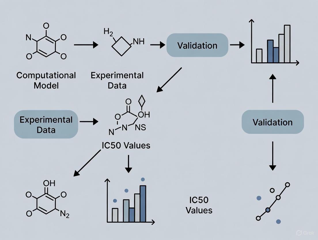
Visualizing the Dynamic Drug Discovery Workflow

The following diagram illustrates the integrated cycle of modern, dynamic approaches to drug discovery that move beyond single-point data.

Dynamic and Integrated Drug Discovery Workflow. This diagram outlines a modern pipeline that uses dynamic computational methods to overcome the limitations of static approaches. Molecular dynamics simulations sample protein flexibility, enabling more effective virtual screening. Promising candidates are evaluated using dynamic resistance models before experimental validation, creating a feedback loop for continuous model improvement.

Advancing Beyond IC50: Superior Metrics and Models

Area Under the Dose-Response Curve (AUDRC)

To address the concentration-range bias inherent in IC50, the Area Under the Dose-Response Curve (AUDRC) is increasingly advocated as a more robust alternative [27]. Unlike IC50, which relies on a single point on the curve, AUDRC integrates the entire dose-response relationship, providing a more comprehensive summary of drug effect across all tested concentrations. This makes it less susceptible to the influence of arbitrary maximum concentration choices and a more reliable label for machine learning models in drug response prediction.

The "Inhibitory Reduction Prowess" Metric

In the specific context of overcoming enzyme-level drug resistance, a novel parameter called "inhibitory reduction prowess" has been proposed [26]. It is defined as the relative decrease in the product formation rate of the target enzyme (e.g., mutant Abl1) in the presence of an inhibitor. Computational models for CML treatment demonstrate that this dynamic metric, which incorporates information on catalysis, inhibition, and pharmacokinetics, is a better indicator of a drug's efficacy against resistant mutants than the traditional fold-IC50 value [26].

The Scientist's Toolkit: Essential Research Reagents and Solutions

Table 2: Key Reagents and Materials for Advanced Drug Potency Studies

Research Reagent / Material	Function in Experimental Protocol
Gold-Coated Nanowire Array Sensors	Serves as the substrate in reflective SPR imaging. Its periodic nanostructure (e.g., 400 nm periodicity) generates a surface plasmon resonance used to detect changes in cell adhesion as a proxy for viability [7].
Molecular Dynamics (MD) Software (e.g., GROMACS, NAMD)	Software suites used to run MD simulations. They calculate the time-dependent behavior of a molecular system (protein-ligand complexes) based on Newtonian physics and specified force fields, revealing dynamics and cryptic pockets [25] [28].
Docking Software (e.g., AutoDock Vina)	Programs that perform molecular docking, predicting the preferred orientation and binding affinity of a small molecule (ligand) to a target macromolecule (receptor) [25]. Often used in conjunction with MD in the Relaxed Complex Scheme [25].
Ultra-Large Virtual Compound Libraries (e.g., REAL Database)	On-demand, synthetically accessible virtual libraries containing billions of drug-like compounds. They dramatically expand the accessible chemical space for virtual screening campaigns, increasing the chance of identifying novel hits [25].
AlphaFold Protein Structure Database	A database providing over 214 million predicted protein structures generated by the machine learning tool AlphaFold. It enables structure-based drug design for targets without experimentally determined 3D structures [25].

The evidence is clear: while the IC50 value offers a convenient and standardized metric for initial compound ranking, its nature as a single-point, static measurement renders it insufficient for navigating the complexities of modern drug discovery, especially in predicting and overcoming drug resistance. The future lies in embracing a multi-faceted and dynamic approach. This paradigm integrates computational techniques like molecular dynamics and the relaxed complex method—which account for the intrinsic flexibility of biological targets—with more informative experimental metrics like AUDRC and innovative, label-free real-time monitoring technologies. Furthermore, the development of novel, mechanism-informed parameters such as "inhibitory reduction prowess" promises to guide treatment selection more effectively in the face of resistance. By moving beyond the IC50-centric view and adopting these integrated strategies, researchers and drug developers can significantly enhance the predictive power of their workflows and accelerate the delivery of more effective and resilient therapeutics.

Methodologies in Action: Techniques for Predicting and Measuring Compound Activity

Structure-based virtual screening has become a cornerstone of early drug discovery, with growing interest in the computational screening of multi-billion compound libraries to identify novel hit molecules [30]. This approach leverages computational power to prioritize compounds for synthesis and testing, dramatically reducing the time and cost associated with traditional experimental high-throughput screening [31]. The success of virtual screening campaigns depends critically on the accuracy of computational docking methods to predict binding poses and affinities, and on the ability to implement these methods at an unprecedented scale [30]. As ultra-large "tangible" libraries containing billions of readily synthesizable compounds become more accessible, robust computational frameworks capable of efficiently screening these vast chemical spaces are increasingly valuable to drug discovery researchers [32]. This guide provides an objective comparison of current platforms and methodologies for large-scale virtual screening, with a specific focus on the experimental validation of computational predictions through binding affinity measurements.

Platform Comparison: Capabilities and Performance

Various computational platforms have been developed to address the formidable challenge of screening billion-compound libraries, each employing distinct strategies to balance speed, accuracy, and computational cost.

Table 1: Comparison of Large-Scale Virtual Screening Platforms

Platform Name	Docking Engine	Scoring Function	Scale Demonstrated	Hit Rate Validation	Computational Infrastructure
RosettaVS (OpenVS)	Rosetta GALigandDock	Physics-based (RosettaGenFF-VS) with entropy	Multi-billion compounds	14% (KLHDC2), 44% (NaV1.7)	HPC (3000 CPUs + GPU), 7 days screening [30]
Schrödinger Virtual Screening Web Service	Glide	Physics-based + Machine Learning	>1 billion compounds	Not specified	Cloud-based, 1 week turnaround [33]
warpDOCK	Qvina2, AutoDock Vina, and others	Vina-based or other compatible functions	100 million+ compounds	Not specified	Oracle Cloud Infrastructure, cost-estimated [34]
DockThor-VS	DockThor	MMFF94S force field + DockTScore	Not specified for ultra-large scale	Not specified	Brazilian SDumont supercomputer [35]

Performance Metrics and Experimental Validation

The ultimate measure of a virtual screening platform's success lies in its ability to identify compounds with experimentally confirmed activity. The RosettaVS platform demonstrated a 14% hit rate against the ubiquitin ligase target KLHDC2 and a remarkable 44% hit rate against the human voltage-gated sodium channel NaV1.7, with all discovered hits exhibiting single-digit micromolar binding affinity [30]. Furthermore, the platform's predictive accuracy was validated by a high-resolution X-ray crystallographic structure that confirmed the docking pose for a KLHDC2-ligand complex [30].

Benchmarking studies provide standardized assessments of docking performance. On the CASF-2016 benchmark, the RosettaGenFF-VS scoring function achieved a top 1% enrichment factor (EF) of 16.72, significantly outperforming other methods [30]. In studies targeting Plasmodium falciparum dihydrofolate reductase (PfDHFR), re-scoring with machine learning-based scoring functions substantially improved performance, with CNN-Score combined with FRED docking achieving an EF1% of 31 against the resistant quadruple-mutant variant [36].

Essential Protocols for Large-Scale Virtual Screening

The RosettaVS Two-Stage Screening Protocol

The RosettaVS method employs a structured workflow to efficiently screen ultra-large libraries while maintaining accuracy.

Figure 1: The two-stage RosettaVS screening workflow with experimental validation. This protocol enables efficient screening of billion-compound libraries while maintaining high accuracy through successive filtering stages.

Protocol Details:

• Virtual Screening Express (VSX) Mode: Initial rapid screening performed with rigid receptor docking to quickly eliminate poor binders from the billion-compound library. This stage prioritizes speed over precision [30].

• Active Learning Compound Selection: A target-specific neural network is trained during docking computations to intelligently select promising compounds for more expensive calculations, avoiding exhaustive docking of the entire library [30].

• Virtual Screening High-Precision (VSH) Mode: A more computationally intensive docking stage that incorporates full receptor flexibility, including side-chain and limited backbone movements, to accurately model induced fit upon ligand binding [30].

• Experimental Validation: Top-ranked compounds proceed to experimental testing, typically beginning with binding affinity measurements (IC50/Kd determination) followed by structural validation through X-ray crystallography when possible [30].

Machine Learning-Enhanced Screening Protocol

An alternative approach integrates machine learning scoring functions with traditional docking tools to improve screening performance, particularly for challenging targets like drug-resistant enzymes.

Protocol Details:

• Initial Docking with Generic Tools: Compounds are initially docked using standard docking programs such as AutoDock Vina, FRED, or PLANTS [36].

• ML-Based Re-scoring: Docking poses are subsequently re-scored using machine learning scoring functions such as CNN-Score or RF-Score-VS v2, which have demonstrated significant improvements in enrichment factors over classical scoring functions [36].

• Enrichment Analysis: Performance is quantified using enrichment factors (EF1%), which measure the ability to identify true actives in the top fraction of ranked compounds, and pROC chemotype analysis to evaluate the diversity of retrieved actives [36].

Successful virtual screening campaigns require careful selection of computational tools, compound libraries, and experimental validation reagents.

Table 2: Essential Research Reagents and Computational Resources for Virtual Screening

Resource Category	Specific Resource	Function and Application	Key Features
Docking Software	Rosetta GALigandDock [30]	Physics-based docking with receptor flexibility	Models side-chain and limited backbone flexibility
	AutoDock Vina [31] [36]	Widely-used docking program	Fast, open-source, good balance of speed and accuracy
	Qvina2 [34]	Docking engine for large-scale screens	Optimized for speed in high-throughput docking
Scoring Functions	RosettaGenFF-VS [30]	Physics-based scoring with entropy estimation	Combines enthalpy (ΔH) and entropy (ΔS) terms
	CNN-Score, RF-Score-VS v2 [36]	Machine learning scoring functions	Improve enrichment when re-scoring docking outputs
Compound Libraries	"Tangible" make-on-demand libraries [32]	Ultra-large screening collections	Billions of synthesizable compounds, increasingly diverse
	ChemDiv Database [37]	Commercial compound library	1.5+ million compounds for initial screening
Experimental Validation Reagents	IC50 Binding Assays [30] [37]	Quantitative binding affinity measurement	Validates computational predictions with experimental data
	X-ray Crystallography [30]	Structural validation of binding poses	Confirms accuracy of predicted ligand binding modes
	Target Protein Structures	Structural basis for docking	Wild-type and mutant forms (e.g., PfDHFR variants) [36]

Key Considerations for Experimental Validation

Correlation Between Computational and Experimental Results

The relationship between computational docking scores and experimental binding affinities forms the critical bridge between in silico predictions and experimental reality. Studies have demonstrated that docking scores typically improve log-linearly with library size, meaning that screening larger libraries increases the likelihood of identifying better-fitting ligands [32]. However, this also increases the potential for false positives that rank artifactually well due to limitations in scoring functions [32].

Experimental validation remains essential, as even the best docking scores represent only approximations of binding affinity. The most convincing validation comes from cases where computational predictions are confirmed through multiple experimental methods, such as binding affinity measurements (IC50) supplemented by high-resolution structural biology approaches like X-ray crystallography [30].

Addressing the Challenge of Novel Chemical Space

Modern ultra-large libraries have significantly expanded the accessible chemical space for drug discovery, but this expansion comes with both opportunities and challenges. Unlike traditional screening collections that show strong bias toward "bio-like" molecules (metabolites, natural products, and drugs), newer billion-compound libraries contain substantially more diverse chemistry, with a 19,000-fold decrease in compounds highly similar to known bio-like molecules [32]. Interestingly, successful hits from large-scale docking campaigns consistently show low similarity to bio-like molecules, with Tanimoto coefficients typically below 0.6 and peaking around 0.3-0.35 [32]. This suggests that effective virtual screening platforms must be capable of identifying novel chemotypes beyond traditional drug-like space.

Virtual screening of billion-compound libraries represents a powerful approach for lead discovery in drug development, with platforms like RosettaVS, Schrödinger's Virtual Screening Web Service, and warpDOCK demonstrating capabilities to efficiently navigate this vast chemical space. The integration of advanced scoring functions, active learning methodologies, and machine learning-based re-scoring has significantly improved the enrichment of true hits from docking screens. Critical to the success of any virtual screening campaign is the rigorous experimental validation of computational predictions through binding affinity measurements and structural biology approaches. As tangible compound libraries continue to expand and computational methods evolve, the ability to effectively leverage these resources will become increasingly important for drug discovery researchers seeking to identify novel chemical starting points for therapeutic development.

In the field of drug discovery and precision oncology, the half-maximal inhibitory concentration (IC50) serves as a crucial quantitative measure of a compound's potency, representing the concentration required to inhibit a biological process by half. Accurate prediction of IC50 values is fundamental for assessing drug efficacy, prioritizing candidate compounds, and tailoring personalized treatment strategies. The advent of large-scale pharmacogenomic databases, such as the Cancer Cell Line Encyclopedia (CCLE) and the Genomics of Drug Sensitivity in Cancer (GDSC), has provided researchers with extensive datasets containing molecular characterizations of cancer cell lines alongside drug sensitivity measurements, enabling the development of machine learning models for IC50 prediction.

Machine learning approaches have dramatically transformed the landscape of drug sensitivity prediction, offering powerful tools to decipher complex relationships between molecular features of cancer cells and their response to therapeutic compounds. These models range from traditional ensemble methods like Random Forests to sophisticated deep neural architectures, each with distinct strengths, limitations, and performance characteristics. The integration of diverse biological data types—including gene expression profiles, mutation data, and chemical compound representations—has further enhanced the predictive capability of these models, advancing their applications in virtual screening, drug repurposing, and personalized treatment recommendation.

This comprehensive comparison guide examines the current state of machine learning approaches for IC50 prediction, providing an objective evaluation of algorithmic performance across multiple experimental settings and datasets. By synthesizing empirical evidence from benchmarking studies and innovative methodological developments, this review offers researchers and drug development professionals a structured framework for selecting appropriate modeling strategies based on specific research objectives, data availability, and performance requirements.

Comparative Performance of Machine Learning Algorithms

Benchmarking Studies and Performance Metrics

Table 1: Performance Comparison of ML Algorithms for IC50 Prediction on GDSC Data

Algorithm	Best-Performing DR Method	Average R²	Average RMSE	Key Strengths	Key Limitations
Elastic Net	PCA, mRMR	0.43	0.64	Lowest runtime, high interpretability, robust to overfitting	Linear assumptions may miss complex interactions
Random Forest	MACCS fingerprints	0.45	0.62	Handles non-linear relationships, robust to outliers	Longer training time, less interpretable than linear models
Boosting Trees	mRMR	0.41	0.67	High predictive power with proper tuning	Prone to overfitting without careful parameter tuning
Neural Networks	PCA	0.38	0.71	Captures complex interactions, flexible architectures	Computationally intensive, requires large data volumes

Large-scale benchmarking studies provide critical insights into the relative performance of machine learning algorithms for IC50 prediction. A comprehensive evaluation of four machine learning algorithms—random forests, neural networks, boosting trees, and elastic net—across 179 anti-cancer compounds from the GDSC database revealed important performance patterns [38]. The study employed nine different dimension reduction techniques to manage the high dimensionality of gene expression data (17,419 genes) and trained models to predict logarithmized IC50 values.

The results demonstrated that elastic net models achieved the best overall performance across most compounds while maintaining the lowest computational runtime [38]. This superior performance of regularized linear models suggests that for many drug response prediction tasks, the relationship between gene expression and IC50 may be sufficiently captured by linear relationships when combined with appropriate feature selection. Random forests consistently displayed robust performance across diverse drug classes, particularly when using MACCS fingerprint representations for drug compounds [39]. The algorithm's ability to handle non-linear relationships and maintain performance with minimal hyperparameter tuning contributes to its widespread adoption in drug sensitivity prediction.

Neural networks generally showed more variable performance, excelling for specific drug classes but demonstrating poorer average performance across the entire compound library [38]. This performance pattern highlights the importance of dataset size and architecture optimization for deep learning approaches, as they typically require larger training samples to reach their full potential compared to traditional machine learning methods.

Domain Adaptation and Cross-Database Performance

Table 2: Cross-Database Model Performance (CCLE to GDSC Transfer)

Model Architecture	RMSE	R²	Key Features	Transfer Strategy
DADSP (Proposed)	0.64	0.43	Domain adversarial discriminator	Domain adaptation
DADSP-A (No pre-training)	0.71	0.31	Standard deep feedforward network	No transfer learning
DeepDSC-1 (Target only)	0.69	0.35	Stacked autoencoder	No source domain data
DeepDSC-2 (With pre-training)	0.66	0.39	Joint pre-training on both domains	Parameter transfer
SLA (Selective Learning)	0.65	0.41	Intermediate domain selection	Selective transfer

The challenge of cross-database prediction represents a significant hurdle in computational drug discovery, as models trained on one dataset often experience performance degradation when applied to external datasets due to technical variations and batch effects. The DADSP (Domain Adaptation for Drug Sensitivity Prediction) framework addresses this challenge through a deep transfer learning approach that integrates gene expression profiles from both CCLE and GDSC databases [40]. This method employs stacked autoencoders for feature extraction and domain adversarial training to align feature distributions across source and target domains, significantly improving cross-database generalization.

Experimental results demonstrate that models incorporating domain adaptation strategies consistently outperform those trained exclusively on target domain data [40]. The DADSP model achieved an RMSE of 0.64 and R² of 0.43 in cross-database prediction tasks, representing approximately 10% improvement in RMSE compared to models without domain adaptation components [40]. This performance advantage highlights the value of transfer learning methodologies in addressing distributional shifts between pharmaceutical databases, a common challenge in computational drug discovery.

Beyond traditional IC50 prediction, recent research has pioneered models capable of predicting complete dose-response curves rather than single summary metrics [41]. The Functional Random Forest (FRF) approach represents a significant methodological advancement by incorporating region-wise response points or distributions in regression tree node costs, enabling prediction of entire dose-response profiles [41]. This functionality provides more comprehensive drug sensitivity characterization beyond IC50 values alone, capturing critical information about drug efficacy across concentration gradients.

Experimental Protocols and Methodologies

Data Preprocessing and Feature Engineering

The foundational step in IC50 prediction involves meticulous data preprocessing and feature engineering to transform raw biological and chemical data into machine-learnable representations. For genomic features, the standard protocol involves normalization of gene expression data to mitigate technical variations between experiments. In the DrugS model framework, researchers implement log transformation and scaling of expression values for 20,000 protein-coding genes to minimize outlier influence and ensure cross-dataset comparability [42]. For chemical compound representation, extended-connectivity fingerprints (ECFPs) and MACCS keys serve as prevalent structural descriptors, capturing molecular substructures and key functional groups relevant to biological activity [39].

Dimensionality reduction represents a critical preprocessing step given the high-dimensional nature of genomic data (typically >17,000 genes) relative to limited cell line samples (typically hundreds to thousands). Benchmarking studies have systematically evaluated various dimension reduction techniques, including principal component analysis (PCA) and minimum-redundancy-maximum-relevance (mRMR) feature selection [38]. Results indicate that feature selection methods incorporating drug response information during feature selection generally outperform methods based solely on expression variance, underscoring the importance of response-guided feature engineering.

The experimental protocol for model development typically involves strict separation of training and test sets at the cell line level, with 80% of cell lines allocated for training and 20% held out for testing [38]. This splitting strategy ensures that model performance reflects generalization to unseen cell lines rather than memorization of training instances. For cross-database validation, additional steps include dataset harmonization to align gene identifiers and expression measurement units between source and target domains [40].

Model Training and Hyperparameter Optimization

The model training phase employs systematic hyperparameter optimization to maximize predictive performance while mitigating overfitting. For tree-based methods including Random Forests and boosting trees, critical hyperparameters include the number of trees in the ensemble, maximum tree depth, and the number of features considered for each split [38]. The benchmarking protocol typically involves 5-fold cross-validation on the training set to evaluate hyperparameter combinations, with the mean squared error (MSE) serving as the primary optimization metric [38].

For neural network architectures, hyperparameter space encompasses the number of hidden layers, activation functions, dropout rates, and learning rate schedules. The DrugS model employs a specialized architecture incorporating autoencoder-based dimensionality reduction to compress 20,000 genes into 30 latent features, which are then concatenated with 2,048 chemical features derived from compound SMILES strings [42]. This approach effectively addresses the "small n, large p" problem prevalent in drug sensitivity prediction, where the number of features vastly exceeds the number of samples.

The Functional Random Forest implementation introduces modified node cost calculations that incorporate the complete dose-response curve structure rather than individual response values [41]. This approach represents functional data using B-spline basis expansions and modifies the node splitting criterion to consider response distributions across concentration gradients, enabling more biologically-informed model training.

Figure 1: Experimental Workflow for IC50 Prediction Models. This diagram illustrates the standard methodology for developing machine learning models to predict drug sensitivity, encompassing data sourcing, preprocessing, model training with cross-validation, and output generation.

Signaling Pathways and Biological Mechanisms

Genomic Determinants of Drug Sensitivity

Machine learning models for IC50 prediction have revealed important insights into the biological mechanisms and signaling pathways that govern drug sensitivity in cancer cells. Gene expression profiles consistently emerge as the most predictive features for drug response across multiple benchmarking studies [38] [42]. Clustering analyses of cancer cell lines based on gene expression patterns reveal distinct molecular subtypes that correlate with differential drug sensitivity, highlighting the fundamental relationship between transcriptional states and therapeutic response [42].

Pathway enrichment analyses of genes selected as important features in predictive models identify several key signaling pathways frequently associated with drug sensitivity mechanisms. These include the PI3K-Akt signaling pathway, TNF signaling pathway, and NF-κB signaling pathway, all of which play critical roles in cell survival, proliferation, and death decisions [42]. Models trained specifically on pathway activity scores rather than individual gene expressions have demonstrated competitive performance while offering enhanced biological interpretability, directly linking predicted sensitivities to dysregulated biological processes.

For targeted therapies, specific genomic alterations serve as strong predictors of sensitivity or resistance. For instance, BRAF V600E mutations predict sensitivity to RAF inhibitors, while HER2 amplification status determines response to HER2-targeted therapies [42]. The integration of mutation data with gene expression profiles further enhances prediction accuracy for molecularly targeted agents, enabling more precise identification of patient subgroups likely to benefit from specific treatments.

Chemical and Structural Determinants of Compound Potency

Beyond cellular features, the chemical properties of compounds significantly influence their biological activity and potency. Molecular fingerprints that encode chemical structure information, particularly MACCS keys and Morgan fingerprints, have proven highly effective in representing compounds for sensitivity prediction [39]. These representations capture structural features relevant to target binding, membrane permeability, and metabolic stability, all of which contribute to compound efficacy.

Studies comparing alternative drug representations, including physico-chemical properties and explicit target information, found that structural fingerprints generally outperformed other representation schemes [39]. This advantage likely stems from their ability to encode complex structural patterns that correlate with biological activity, enabling models to identify structural motifs associated with potency against specific cancer types.

Figure 2: Key Signaling Pathways in Drug Sensitivity Mechanisms. This diagram illustrates the relationship between dysregulated cancer pathways, drug classes, and their mechanisms of action, highlighting biological processes that influence IC50 values.

Research Reagent Solutions and Computational Tools

Table 3: Essential Research Resources for IC50 Prediction Studies

Resource Category	Specific Resource	Key Application	Access Information
Pharmacogenomic Databases	GDSC	Drug sensitivity data for 700+ cell lines	https://www.cancerrxgene.org
	CCLE	Molecular characterization of 1000+ cell lines	https://sites.broadinstitute.org/ccle
	DrugComb	Harmonized drug combination screening data	https://drugcomb.org
Chemical Databases	ChEMBL	Bioactivity data for drug-like molecules	https://www.ebi.ac.uk/chembl
	PubChem	Chemical structures and properties	https://pubchem.ncbi.nlm.nih.gov
Software Libraries	scikit-learn	Traditional ML algorithms (RF, EN)	https://scikit-learn.org
	TensorFlow/Keras	Deep neural network implementation	https://www.tensorflow.org
	caret	Unified framework for model training	https://topepo.github.io/caret

The development and validation of IC50 prediction models rely on specialized computational tools and data resources that enable reproducible research. Pharmacogenomic databases serve as foundational resources, providing comprehensive drug sensitivity measurements alongside molecular characterization data. The GDSC database contains sensitivity data for 198 drugs across approximately 700 cancer cell lines, while the CCLE provides complementary data for 947 cell lines and 24 compounds [41]. The recently established DrugComb portal further expands these resources by aggregating harmonized drug combination screening data from 37 sources, enabling development of models for combination therapy response [39].

For chemical data representation, resources including ChEMBL and PubChem provide standardized compound structures and bioactivity data essential for training structure-activity relationship models. The integration of Simplified Molecular Input Line Entry System (SMILES) representations with molecular fingerprinting algorithms enables efficient encoding of chemical structures for machine learning applications [42]. Specialized packages like RDKit offer comprehensive cheminformatics functionality for fingerprint generation, molecular descriptor calculation, and chemical similarity assessment.

Machine learning libraries provide the algorithmic implementations necessary for model development. The scikit-learn library in Python offers efficient implementations of traditional algorithms including random forests and elastic net, while TensorFlow and Keras support development of deep neural architectures [38]. For R users, the caret package provides a unified interface for multiple machine learning algorithms with streamlined preprocessing and hyperparameter tuning capabilities [38]. These tools collectively establish a robust software ecosystem for developing, validating, and deploying IC50 prediction models.

The comprehensive comparison of machine learning approaches for IC50 prediction reveals a complex performance landscape where no single algorithm dominates across all scenarios. Elastic net regression demonstrates exceptional performance for many drug prediction tasks despite its relative simplicity, offering advantages in computational efficiency, interpretability, and robustness to overfitting [38]. Random forest models maintain strong performance across diverse experimental conditions, particularly when combined with appropriate chemical structure representations [39]. More complex deep neural architectures show promise for specific applications but require careful architecture design and substantial training data to achieve their full potential [42].

The evolution of IC50 prediction is moving beyond single summary metrics toward complete dose-response curve prediction [41]. Functional Random Forest approaches represent an important step in this direction, enabling prediction of response across concentration gradients rather than isolated IC50 values. This paradigm shift provides more comprehensive characterization of compound potency and efficacy, supporting more informed therapeutic decisions. Similarly, the development of models capable of predicting combination therapy response addresses a critical clinical need, as drug combinations increasingly represent standard care across multiple cancer types [39].

Future advancements in IC50 prediction will likely focus on improved generalization across datasets through enhanced domain adaptation techniques [40], integration of multi-omics data beyond transcriptomics, and development of interpretable models that provide biological insights alongside predictions. As these models continue to mature, their integration into drug discovery pipelines and clinical decision support systems holds significant promise for accelerating therapeutic development and personalizing cancer treatment.

In modern computational drug discovery, the representation of a chemical molecule is a fundamental determinant of the success of predictive models. The process of feature engineering—selecting and optimizing how molecules are translated into numerical vectors—lies at the heart of building reliable Quantitative Structure-Activity Relationship (QSAR) models. These models aim to predict biological activity, such as the half-maximal inhibitory concentration (IC₅₀), from chemical structure. Within the broader thesis of validating computational predictions with experimental IC₅₀ values, understanding the strengths and limitations of different molecular representations is paramount for researchers and drug development professionals. This guide provides an objective comparison of the two primary families of molecular representations—molecular descriptors and structural fingerprints—by examining their performance across various experimental protocols and biological targets.

Molecular representations can be broadly classified into two categories: molecular descriptors and structural fingerprints.

• Molecular Descriptors are often calculated from the molecular structure and represent global physicochemical properties. Examples include molecular weight (MolWt), topological polar surface area (TPSA), and the octanol-water partition coefficient (logP) [43] [44]. They are typically continuous numerical values and are classified by the dimensionality of the information they encode (e.g., 1D, 2D, or 3D) [44].
• Structural Fingerprints are typically binary or count-based vectors that encode the presence or absence of specific substructures or topological patterns within the molecule [45]. Key types include:
  • Circular Fingerprints (e.g., ECFP, FCFP, Morgan): These generate molecular features by iteratively considering the neighborhood around each atom up to a certain radius, creating a representation that captures local chemical environment [45] [46].
  • Path-based Fingerprints (e.g., Atom Pairs, Topological Torsions): These analyze paths through the molecular graph, recording features based on atom pairs or sequences of connected bonds [45] [47].
  • Substructure Key-based Fingerprints (e.g., MACCS Keys): These use a predefined dictionary of structural fragments, where each bit in the vector corresponds to the presence or absence of one specific fragment [45] [46].

The choice between descriptors and fingerprints is not merely technical; it influences the model's interpretability, its ability to generalize, and ultimately, how well its predictions can be validated with experimental IC₅₀ assays.

Performance Comparison Across Benchmarks

Predictive Performance in Various Biological Contexts

Extensive benchmarking studies have evaluated these representations across diverse prediction tasks. The following table summarizes key performance metrics from recent research.

Table 1: Comparative Performance of Molecular Representations on Different Prediction Tasks

Prediction Task	Best Performing Representation	Algorithm	Key Performance Metric(s)	Source / Context
Odor Perception	Morgan Fingerprints (ST)	XGBoost	AUROC: 0.828; AUPRC: 0.237 [43]	Curated dataset of 8,681 compounds [43]
ADME-Tox Targets(e.g., Ames, hERG, BBB)	Traditional 2D Descriptors	XGBoost	Superior to fingerprints for most targets [44]	Literature-based datasets (1,000-6,500 molecules) [44]
Drug Combination Sensitivity & Synergy	Data-Driven & Rule-Based Fingerprints (variable)	Multiple ML/DL models	Performance context-dependent [48]	14 drug screening studies; 4153 molecules [48]
Natural Products Bioactivity	Extended Connectivity Fingerprints (ECFP) & others	N/A	Matched or outperformed other fingerprints [45]	12 QSAR datasets from CMNPD [45]
Virtual Screening (Similarity Search)	ECFP4 / ECFP6 & Topological Torsions	Similarity-based	Top performance for ranking diverse structures [47]	Literature-based similarity benchmark [47]

Analysis of Comparative Data

The data reveals that no single representation is universally superior. The Morgan (ECFP) fingerprint consistently ranks among the top performers for a wide range of tasks, particularly in odor prediction and virtual screening, due to its ability to capture relevant local structural features without relying on pre-defined fragments [43] [47]. However, in specific contexts like ADME-Tox prediction, traditional 2D molecular descriptors can outperform even the most popular fingerprints, suggesting that global physicochemical properties are highly informative for these endpoints [44]. This underscores the importance of task-specific feature selection in the process of validating computational models.

Detailed Experimental Protocols for Performance Validation

To ensure the reliability of comparative data, the cited studies employed rigorous and standardized experimental protocols.

Protocol 1: Benchmarking Fingerprints for Odor Decoding

This protocol outlines the methodology used to establish the superior performance of Morgan fingerprints for odor prediction [43].

• 1. Dataset Curation: A unified dataset of 8,681 unique odorants was assembled from ten expert-curated sources. Odor descriptors were standardized into a controlled set of 201 labels to ensure consistency [43].
• 2. Feature Extraction: Three feature sets were generated for each molecule:
  • Functional Group (FG) Fingerprints: Based on predefined substructures using SMARTS patterns.
  • Molecular Descriptors (MD): Calculated using RDKit, including MolWt, TPSA, and logP.
  • Morgan Structural Fingerprints (ST): Generated from molecular representations using the Morgan algorithm [43].
• 3. Model Training & Evaluation: Three tree-based algorithms (Random Forest, XGBoost, and LightGBM) were trained for each feature set. Models were evaluated using stratified 5-fold cross-validation, with performance measured by Area Under the Receiver Operating Characteristic Curve (AUROC) and Area Under the Precision-Recall Curve (AUPRC) [43].

Protocol 2: Evaluating Representations for ADME-Tox Targets

This protocol details the comparison that demonstrated the competitiveness of traditional descriptors in ADME-Tox modeling [44].

• 1. Dataset Curation: Six medium-sized, literature-based binary classification datasets (e.g., Ames mutagenicity, hERG inhibition) were curated, each containing over 1,000 molecules. A standardized filtering protocol was applied, including salt removal and element filtering [44].
• 2. Feature Extraction: Five molecular representation sets were compared:
  • Fingerprints: MACCS, Atompairs, Morgan.
  • Descriptors: Traditional 1D & 2D descriptors, and 3D molecular descriptors [44].
• 3. Model Training & Evaluation: Two distinct algorithms, XGBoost and RPropMLP (a neural network), were used for model building. A comprehensive statistical evaluation based on 18 different performance parameters was conducted to ensure robust conclusions [44].

Advanced Strategies: Hybrid and Conjoint Approaches

Given the complementary strengths of different representations, advanced strategies have emerged to leverage their combined power.

• Conjoint Fingerprints: Research has shown that simply combining two complementary fingerprints into a single conjoint fingerprint vector can yield improved predictive performance. This approach leverages the automatic feature engineering capability of deep learning models to harness the supplementary information captured by different fingerprint types, even outperforming consensus models in some cases [49].
• Data-Driven Fingerprints: Modern deep learning methods, such as Graph Neural Networks (GNNs) and autoencoders, can generate data-driven fingerprints. These models learn optimal molecular representations directly from the data, such as from molecular graphs or SMILES strings, often capturing complex patterns that are not explicitly defined in rule-based fingerprints [48] [50] [46]. For instance, one study developed a natural product-specific "neural fingerprint" using an artificial neural network, which outperformed traditional fingerprints in virtual screening tasks [50].

The following diagram illustrates the workflow for developing and applying a conjoint fingerprint strategy.

The Scientist's Toolkit: Essential Research Reagents & Materials

The following table lists key software tools and resources essential for conducting feature engineering and model validation in computational drug discovery.

Table 2: Key Research Reagent Solutions for Molecular Feature Engineering

Tool / Resource Name	Type	Primary Function in Feature Engineering	Relevant Citation
RDKit	Open-source Cheminformatics Library	Calculates molecular descriptors, generates fingerprints (e.g., Morgan), and handles molecular standardization.	[43] [44] [46]
PubChem	Public Chemical Database	Source for canonical SMILES strings and chemical identifiers via its PUG-REST API.	[43] [46]
Python pyrfume-data	GitHub Archive	Provides access to unified, curated olfactory datasets for model training and validation.	[43]
ChEMBL	Manual Bioactivity Database	Source of curated bioactivity data (e.g., IC50) for building benchmark datasets.	[48] [47]
DeepChem	Open-source Deep Learning Library	Provides tools for generating neural fingerprints and graph-based molecular features.	[46]
Schrödinger Suite	Commercial Software	Used for advanced molecular modeling tasks, including geometry optimization for 3D descriptor calculation.	[44]
DrugComb Portal	Public Database	Source of standardized drug combination sensitivity and synergy data for benchmarking.	[48]

Decision Framework for Representation Selection

The following flowchart provides a structured guide for researchers to select the most appropriate molecular representation for their specific project goals, based on the empirical evidence presented.

The empirical evidence clearly demonstrates that the choice between molecular descriptors and structural fingerprints is not a matter of one being universally better than the other. Instead, the optimal feature engineering strategy is highly context-dependent. Morgan fingerprints and other circular topological representations have proven to be robust and powerful general-purpose tools [43] [47]. However, for targets where holistic physicochemical properties are highly informative, such as ADME-Tox endpoints, traditional molecular descriptors remain fiercely competitive [44]. The emerging paradigms of conjoint fingerprints and data-driven representations offer promising paths to overcome the limitations of standalone featurization by harnessing complementary information [49] [46]. For researchers focused on validating computational predictions with experimental IC₅₀ values, a prudent approach is to empirically benchmark multiple representation types on a relevant, well-curated dataset, as this remains the most reliable method to ensure predictive accuracy and model robustness.

In drug discovery, the half-maximal inhibitory concentration (IC50) is a crucial quantitative measure of a substance's potency for inhibiting a specific biological or biochemical function by 50% in vitro [1]. This parameter serves as an essential experimental benchmark for validating computational predictions, bridging the gap between in silico models and empirical biological activity [51]. As research increasingly relies on computer-aided drug design and machine learning to identify novel compounds, experimental determination of IC50 values provides the critical ground truth needed to assess predictive model accuracy and refine computational approaches [51]. The reliability of these experimental measurements directly impacts the success of rational drug design efforts, making robust assay design and execution fundamental to advancing therapeutic development.

Foundational Principles of IC50

Definition and Theoretical Framework

IC50 represents the molar concentration of an inhibitor required to reduce a given biological activity by half [1]. It is an operational parameter dependent on specific assay conditions rather than an absolute physical constant [52]. This distinguishes it from the inhibition constant (Ki), which is an intrinsic thermodynamic property reflecting the affinity of an inhibitor for its target [1]. The relationship between IC50 and Ki can be mathematically described using the Cheng-Prusoff equation for competitive inhibitors: Ki = IC50 / (1 + [S]/Km), where [S] is the substrate concentration and Km is the Michaelis constant [1]. This relationship highlights how IC50 values vary with experimental conditions, while Ki remains constant for a given inhibitor-target interaction.

Researchers sometimes convert IC50 values to the pIC50 scale (pIC50 = -log10(IC50)), where higher values indicate exponentially more potent inhibitors [1]. This transformation is particularly useful for statistical analyses and machine learning applications, as it creates a more normally distributed variable for modeling structure-activity relationships [51].

Comparison of IC50 and Related Potency Measures

Different potency measurements serve distinct purposes in pharmacological research. The table below compares key metrics:

Potency Measure	Full Name	Definition	Application Context
IC50	Half Maximal Inhibitory Concentration	Concentration required for 50% inhibition of a biological process [1]	Antagonist drugs; enzyme inhibitors; cellular toxicity studies
EC50	Half Maximal Effective Concentration	Concentration required to elicit 50% of a maximum effect [1]	Agonist drugs; activators; stimulatory compounds
Ki	Inhibition Constant	Equilibrium dissociation constant for inhibitor binding [1]	Direct measure of binding affinity, independent of assay conditions

Experimental Methodologies for IC50 Determination

Functional Assays in Cellular Systems

Functional antagonist assays determine IC50 by constructing a dose-response curve that examines how different concentrations of an antagonist reverse agonist activity [1]. The concentration needed to inhibit half of the maximum biological response of the agonist is reported as the IC50 [1]. In cellular contexts such as cancer research, these assays typically measure cell viability or metabolic activity in response to drug treatment. For example, studies on CL1-0 and A549 lung cancer cells, Huh-7 liver cancer cells, and MCF-7 breast cancer cells have used various detection methods to quantify cytotoxicity and determine IC50 values for anticancer drugs like doxorubicin [7].

The experimental workflow for cellular IC50 determination involves several standardized steps as illustrated below:

Competition Binding Assays

Competition binding assays provide an alternative approach for IC50 determination, particularly useful for characterizing receptor-ligand interactions [1]. In this format, a single concentration of radioligand (typically at or below its Kd value) is incubated with the target in the presence of varying concentrations of the test inhibitor [1]. The IC50 in this context is defined as the concentration of competing ligand that displaces 50% of the specific binding of the radioligand [1]. This value is then converted to an absolute inhibition constant Ki using the Cheng-Prusoff equation, providing a more fundamental measure of binding affinity [1].

Advanced Label-Free Detection Methods

Recent technological advances have introduced label-free methods for IC50 determination that overcome limitations of traditional endpoint assays. Surface Plasmon Resonance (SPR) imaging represents one such innovation, enabling real-time, non-invasive monitoring of cellular responses without fluorescent labels or dyes [7]. This approach detects changes in cell adhesion and morphology—early indicators of apoptosis and necrosis—through nanostructure-enhanced sensors [7].

The SPR imaging platform utilizes gold-coated periodic nanowire array sensors with a 400 nm periodicity, producing a reflective SPR dip at 580 nm [7]. Differential SPR response is captured through contrast imaging of red and green channels, reflecting changes in cell adhesion strength in response to compound treatment [7]. Studies demonstrate that IC50 values derived from SPR imaging closely align with those obtained via traditional cell staining methods, while offering advantages including continuous monitoring, avoidance of assay interference, and preservation of live cells for downstream analysis [7].

Research Reagent Solutions for IC50 Assays

Successful IC50 determination requires carefully selected reagents and materials. The following table outlines essential solutions for reliable experimental outcomes:

Reagent/Material	Function	Application Notes
Tetrazolium Salts (e.g., MTT, CCK-8)	Measure metabolic activity via intracellular dehydrogenase enzymes [7]	CCK-8 may fail for certain cell types (e.g., MCF-7); potential interference with reducing agents [7]
Cell Staining Dyes	Direct visualization of viable/dead cells [7]	Aligns well with SPR-derived IC50 values; requires fixation and may be endpoint only [7]
SPR Biosensor Chips	Label-free detection of cell adhesion changes [7]	Gold-coated nanowire arrays; enable real-time kinetic monitoring of cytotoxicity [7]
Radioligands	Traceable binding molecules for competition assays [1]	Used at concentrations ≤ Kd; require specialized handling and safety precautions [1]

Data Analysis and Quality Control for Reliable IC50 Estimation

Curve Fitting and Parameter Estimation

Accurate IC50 estimation requires appropriate curve fitting methodologies. The 4-parameter logistic model is commonly employed, which describes the sigmoidal relationship between inhibitor concentration and response [53]. This model provides estimates of the lower and upper plateaus, the slope factor (Hill coefficient), and the relative IC50—defined as the parameter c in the model, representing the concentration corresponding to a response midway between the estimated lower and upper plateaus [53].

For assays with stable 100% controls, the absolute IC50 may be used, defined as the concentration corresponding to the 50% control (the mean of the 0% and 100% assay controls) [53]. The decision to use relative versus absolute IC50 should be based on assay performance characteristics: assays without stable 100% controls must use the relative IC50, while those demonstrating accurate and stable 100% controls with less than 5% error in the estimate of the 50% control mean may benefit from the absolute IC50 approach [53].

Key Validation Parameters for IC50 Assays

The following diagram illustrates the critical decision points for generating reliable IC50 data:

Guidelines for Reportable IC50 Values

To ensure confidence in IC50 estimates, specific requirements must be met regarding the concentration-response relationship:

• For relative IC50: The assay should include at least two concentrations beyond the lower and upper bend points of the sigmoidal curve [53]
• For absolute IC50: There should be at least two assay concentrations whose predicted response is less than 50% and two whose predicted response is greater than 50% [53]

These criteria ensure adequate characterization of the complete concentration-response relationship, preventing extrapolation beyond the measured data range and providing sufficient information for accurate curve fitting.

Comparative Analysis of IC50 Determination Methods

Different methodological approaches offer distinct advantages and limitations for IC50 determination. The table below provides a comparative overview:

Method	Key Principles	Advantages	Limitations
Functional Cellular Assays	Measures biological response in live cells [1]	Physiological relevance; accounts for cellular uptake and metabolism	Compound interference with detection; endpoint measurement only in traditional formats
Competition Binding Assays	Displacement of radioligand from target [1]	Direct measurement of target engagement; converts to Ki via Cheng-Prusoff [1]	May not reflect functional activity; requires specialized radioactive handling
SPR Imaging	Label-free detection of cell adhesion changes [7]	Real-time kinetic data; no labels or interference; works with difficult cell types [7]	Specialized equipment required; higher initial cost; data interpretation complexity
Traditional Enzymatic Assays	Colorimetric or fluorescent readout of enzyme activity [7]	Simple, cost-effective; amenable to high-throughput screening	Susceptible to compound interference; limited to enzymatic targets; endpoint only

Reliable experimental IC50 data serves as the cornerstone for validating and refining computational predictions in drug discovery. As machine learning approaches increasingly contribute to identifying novel therapeutic compounds [51], the quality of experimental training data becomes paramount. By implementing robust assay methodologies, adhering to rigorous validation criteria, and selecting appropriate detection technologies, researchers can generate high-quality IC50 values that effectively bridge computational predictions and biological reality. This integration accelerates the development of safer, more effective therapeutics through iterative cycles of prediction and experimental validation.

Alzheimer's disease (AD) stands as the most prevalent form of dementia, affecting over 50 million individuals globally, with projections rising to 152 million by 2050 [54]. The complex, multifactorial pathogenesis of AD, characterized by multiple pathological processes including β-amyloid (Aβ) deposits, tau protein aggregation, acetylcholine deficiency, oxidative stress, and neuroinflammation, has rendered single-target therapeutic approaches largely ineffective [55] [56]. This recognition has catalyzed a paradigm shift in drug discovery toward multi-target-directed ligands (MTDLs) designed to address several pathological mechanisms simultaneously [55]. The dual-target drug development strategy offers unique advantages: it can synergistically enhance therapeutic efficacy beyond what single-target drugs can achieve while potentially reducing side effects associated with high doses of single-target agents or drug combinations [55].

Among the various target combinations being explored, dual inhibitors targeting acetylcholinesterase (AChE) alongside other key enzymes have emerged as particularly promising. AChE plays a crucial role in nerve conduction by hydrolyzing acetylcholine (ACh) at synaptic junctions, and AChE inhibitors represent one of the primary therapeutic strategies for ameliorating cholinergic deficit in AD patients [55]. This case study examines the successful identification and validation of a novel dual inhibitor, with particular emphasis on the integration of computational predictions and experimental validation that exemplifies modern AD drug discovery.

Featured Dual Inhibitor: DKS Series Targeting GSK-3β and BuChE

Lead Compound Identification and Rational Design

A compelling example of contemporary dual inhibitor development comes from research on compounds simultaneously targeting glycogen synthase kinase 3β (GSK-3β) and butyrylcholinesterase (BuChE) [57]. GSK-3β is a serine/threonine kinase critically involved in tau protein phosphorylation, which leads to neurofibrillary tangle formation, while BuChE plays a significant role in hydrolyzing acetylcholine, with its activity increasing as AD progresses [57].

Researchers employed a structure-based drug design approach using scaffold hopping and molecular hybridization methodologies [57]. The design strategy focused on merging structural elements from tacrine (an established cholinesterase inhibitor) and adamantane derivatives, creating hybrid ligands with dual pharmacological activities. This approach involved constructing substantial molecules using linkers, conferring upon a single molecular entity the ability to manifest two discrete pharmacological activities [57].

Computational Validation and Binding Analysis

Through molecular docking studies using AutoDock Vina, researchers identified two standout compounds from their designed series:

Table 1: Computational Binding Profiles of Lead DKS Compounds

Compound	Molecular Targets	Docking Energy (kcal/mol)	Key Interacting Residues
DKS1	GSK-3β	-9.6	Lys85, Val135, Asp133, Asp200
DKS4	BuChE	-12.3	His438, Ser198, Thr120

Compound DKS1 exhibited exceptional binding interactions within the active site of GSK-3β, while DKS4 showed strong affinity for BuChE [57]. These interactions with critical catalytic residues suggested robust inhibitory potential against both enzymatic targets.

Molecular dynamics simulations spanning 100 nanoseconds further confirmed the robust stability of both DKS1 and DKS4 within their respective target binding pockets [57]. The simulations demonstrated maintained ligand-protein interactions throughout the trajectory, with minimal structural deviations, indicating stable binding complexes—a crucial predictor of effective enzyme inhibition.

Experimental Validation and IC50 Determination

The transition from computational prediction to experimental validation represents a critical phase in dual inhibitor development. For the DKS series, this involved comprehensive pharmacological profiling:

Table 2: Experimental ADMET Profile of Lead DKS Compound

Parameter	DKS5 Profile	Significance in Drug Development
Human Oral Absorption	79.792%	Favorable for oral administration
CNS Permeability	High	Essential for brain target engagement
Metabolic Stability	Promising	Reduced risk of rapid clearance

The lead candidate DKS5 exhibited an outstanding human oral absorption rate of 79.792%, surpassing the absorption rates observed for other molecules in the study [57]. This favorable pharmacokinetic profile, combined with its dual inhibitory action, positions such compounds as promising candidates for further development.

Methodological Framework: Integrated Computational-Experimental Workflow

Computational Protocol for Dual Inhibitor Discovery

The successful identification of dual inhibitors relies on a systematic workflow integrating multiple computational and experimental approaches:

Target Selection and Rationale: The combination of GSK-3β and BuChE represents a strategic approach addressing both tau pathology (through GSK-3β inhibition) and cholinergic deficits (through BuChE inhibition) [57]. This synergistic target selection is crucial, as co-targeting these pathways can potentially modify disease progression while enhancing cognitive function.

Structure-Based Molecular Design: Researchers utilized molecular hybridization techniques, fusing tacrine and adamantane pharmacophores to create novel chemical entities with dual-target potential [57]. The hybrid ligand approach extends a distinctive prospect for synthesizing compounds with heightened therapeutic potential by integrating two pharmacologically active constituents.

Molecular Docking and Dynamics: Docking studies against crystal structures of GSK-3β (PDB: 4PTC) and BuChE (PDB: 4BDS) provided initial binding affinity assessments [57]. Subsequent molecular dynamics simulations using Desmond over 100 nanoseconds evaluated the stability of ligand-protein complexes, with principal component analysis (PCA) reducing trajectory dimensionality to confirm binding stability.

Diagram 1: Integrated workflow for dual inhibitor development, showing the iterative computational and experimental phases.

Experimental Validation Protocols

Enzyme Inhibition Assays: Standard protocols for determining half-maximal inhibitory concentration (IC50) values against both target enzymes provide quantitative measures of inhibitory potency. These assays typically involve incubating various concentrations of the test compound with the target enzyme and corresponding substrate, followed by measurement of residual enzyme activity.

Cellular Models and Toxicity Screening: Cell-based assays using neuronal cell lines or primary cultures assess compound effects in more physiologically relevant systems. Cytotoxicity assays (e.g., MTT, LDH) determine therapeutic indices, while mechanistic studies evaluate target engagement in cellular contexts.

ADMET Profiling: Comprehensive absorption, distribution, metabolism, excretion, and toxicity (ADMET) predictions using tools like QikProp and SwissADME provide early indications of drug-likeness [57] [58]. Critical parameters include human oral absorption, blood-brain barrier permeability, metabolic stability, and cytochrome P450 inhibition profiles.

Comparative Analysis with Alternative Dual-Target Strategies

The field of dual-target AD therapeutics encompasses multiple target combinations, each with distinct mechanistic rationales:

Table 3: Comparative Analysis of Dual-Target Strategies in Alzheimer's Disease

Target Combination	Mechanistic Rationale	Research Stage	Advantages	Challenges
AChE/MAO-B [55] [54]	Enhances cholinergic transmission while reducing oxidative stress	Multiple compounds in preclinical development	Addresses multiple neurotransmitter systems	Potential for off-target effects
AChE/GSK-3β [55]	Combats cholinergic deficit and tau hyperphosphorylation	Advanced preclinical studies	Potential to modify tau pathology	Complex chemical optimization
GSK-3β/BuChE [57]	Targets tau and cholinergic pathways simultaneously	Lead optimization	May benefit moderate-severe AD	Balancing target selectivity
AChE/PDE [55]	Increases acetylcholine and second messenger levels	Early preclinical validation	Novel mechanism of action	Unclear efficacy in clinical populations

The diversity of target combinations reflects the multifactorial nature of AD pathology and underscores the importance of target selection based on compelling biological rationale. The GSK-3β/BuChE combination is particularly relevant for disease modification, as it addresses both the protein phosphorylation abnormalities underlying neurofibrillary tangle formation and the neurotransmitter deficits contributing to cognitive symptoms.

The Scientist's Toolkit: Essential Research Reagents and Solutions

Successful development of dual inhibitors requires specialized research tools and methodologies:

Table 4: Essential Research Reagents for Dual Inhibitor Development

Reagent/Resource	Function in Research	Application Examples
Target Enabling Packages (TEPs) [59]	Provide validated tools for understudied targets	Include purified proteins, antibodies, knockout cell lines
3D Protein Structures [57] [58]	Enable structure-based drug design	GSK-3β (PDB: 4PTC), BuChE (PDB: 4BDS)
Validated Antibodies [59]	Target detection and quantification	Western blot, immunohistochemistry applications
Molecular Modeling Software [60] [57]	Computational screening & design	AutoDock Vina, Schrödinger Suite, SYBYL-X
Specialized Cell Assays [61]	Target engagement & toxicity assessment	sCLU AlphaLISA, cytotoxicity assays
ADMET Prediction Platforms [58] [62]	Early pharmacokinetic assessment	SwissADME, PKCSM, QikProp

The emergence of Target Enabling Packages (TEPs) has been particularly valuable for accelerating research on novel or understudied targets [59]. These openly available resources provide validated reagents including purified proteins, antibodies, and gene-edited cell lines that meet stringent quality criteria, reducing barriers to target validation and drug discovery.

Pathway Diagrams: Dual-Target Engagement in Alzheimer's Pathology

The therapeutic rationale for dual GSK-3β/BuChE inhibitors can be visualized through their simultaneous effects on key AD pathological processes:

Diagram 2: Dual-target engagement mechanism showing simultaneous inhibition of BuChE (enhancing acetylcholine signaling) and GSK-3β (reducing tau hyperphosphorylation) to ameliorate cognitive deficits in Alzheimer's disease.

The successful identification of dual GSK-3β/BuChE inhibitors exemplifies the power of integrated computational and experimental approaches in addressing the multifactorial pathology of Alzheimer's disease. The strategic combination of structure-based design, molecular hybridization, and rigorous validation represents a template for future therapeutic development in complex neurodegenerative disorders.

As the field advances, several key developments are shaping the future of dual inhibitor research: (1) the application of artificial intelligence and machine learning to identify novel target combinations and optimize molecular structures [60]; (2) the implementation of open science initiatives and target enabling packages to accelerate validation of novel targets [59]; and (3) the refinement of biomarker strategies to identify patient populations most likely to respond to specific target combinations [63].

The continued diversification of the AD drug development pipeline, which currently includes 138 drugs in clinical trials addressing 15 distinct disease processes, reflects growing recognition that effective AD treatment will likely require simultaneous modulation of multiple pathological pathways [63]. Dual inhibitors represent a promising strategic approach in this evolving therapeutic landscape, offering the potential for enhanced efficacy through synergistic mechanisms while maintaining favorable pharmacokinetic and safety profiles.

Navigating Pitfalls: Strategies for Robust and Generalizable Models

In the field of computational drug discovery, overfitting represents one of the most pervasive and deceptive pitfalls, creating models that perform exceptionally well on training data but fail to generalize to real-world scenarios or unseen data [64]. This undesirable machine learning behavior occurs when a model gives accurate predictions for training data but not for new data, rendering it ineffective for practical applications in drug development [65]. While overfitting is often attributed to excessive model complexity, it is frequently the result of inadequate validation strategies, faulty data preprocessing, and biased model selection—problems that can inflate apparent accuracy and compromise predictive reliability [64]. For researchers working with experimental IC50 values and other bioactivity metrics, the implications of overfitting are particularly severe, potentially leading to misguided lead optimization decisions and costly experimental follow-ups based on unreliable computational predictions.

The central challenge lies in the fact that overfit models experience high variance—they give accurate results for the training set but not for the test set, whereas underfit models experience high bias, giving inaccurate results for both training and test data [65]. Data scientists aim to find the "sweet spot" between underfitting and overfitting when fitting a model, seeking a well-fitted model that can quickly establish the dominant trend for both seen and unseen data sets [65]. This balance becomes especially critical in chemogenomics analysis, where public biochemical IC50 data are often assay-specific and comparable only under certain conditions [8].

Understanding Overfitting: Causes and Manifestations

Root Causes of Overfitting

Overfitting occurs when a machine learning model cannot generalize and fits too closely to the training dataset instead. This problematic behavior arises from several common scenarios:

• The training data size is too small and does not contain enough data samples to accurately represent all possible input data values [65]
• The training data contains large amounts of irrelevant information, called noisy data [65]
• The model trains for too long on a single sample set of data [65]
• The model complexity is high, causing it to learn the noise within the training data rather than the underlying signal [65]

In essence, overfitting causes the model to "memorize" the training data, rather than learning the underlying patterns that generalize to new datasets [66]. This memorization occurs when the model's complexity approaches or surpasses that of the data, causing the model to overadapt to the context of the training set [67].

Examples of Overfitting in Drug Discovery Contexts

The consequences of overfitting manifest differently across computational drug discovery applications:

• Image Analysis Failures: A model trained to identify dogs in photos that was trained predominantly on images of dogs in parks may learn to use grass as a feature for classification and fail to recognize dogs inside rooms [65]
• Prediction Bias: An algorithm predicting student academic performance trained only on candidates from a specific gender or ethnic group will experience dropped accuracy for candidates outside these demographics [65]
• Bioactivity Prediction Errors: Models predicting drug-target binding affinities may appear accurate on training data but fail to generalize to new chemical scaffolds or protein variants [18]

Validation Strategies: Comparative Analysis of Methods

Robust validation is the cornerstone of detecting and preventing overfitting. Different validation approaches offer varying levels of protection against overfitting, with appropriate selection depending on dataset size, model complexity, and available computational resources.

Table 1: Comparison of Validation Methods for Detecting Overfitting

Validation Method	Key Principle	Advantages	Limitations	Best Suited For
Train-Test Split (Hold-out) [68]	Splits data into training and testing sets (e.g., 80%-20%)	Simple to implement; computationally efficient	Performance depends on single random split; reduces data for training	Large datasets with sufficient samples
K-Fold Cross-Validation [65]	Divides data into K subsets; iteratively uses each as validation	Uses all data for training and validation; more reliable performance estimate	Computationally expensive; requires careful setup to avoid data leakage	Medium-sized datasets; hyperparameter tuning
Stratified Cross-Validation [66]	Maintains class distribution proportions across folds	Preserves important data characteristics; better for imbalanced datasets	Increased implementation complexity	Classification with imbalanced classes
Leave-One-Out Cross-Validation (LOOCV) [66]	Uses single observation as validation and remainder as training	Maximizes training data; nearly unbiased estimate	Computationally prohibitive for large datasets	Very small datasets

Advanced Validation Considerations for Bioactivity Data

For researchers working with experimental IC50 values, specialized validation considerations apply. The standard deviation of public ChEMBL IC50 data is greater than the standard deviation of in-house intra-laboratory/inter-day IC50 data, highlighting the additional variability introduced when combining data from different sources and experimental conditions [8]. When mixing public IC50 data from different assays, studies have found that this practice "only adds a moderate amount of noise to the overall data," with the standard deviation of IC50 data being only 25% larger than the standard deviation of Ki data [8]. Furthermore, augmenting mixed public IC50 data by public Ki data does not deteriorate the quality of the mixed IC50 data if the Ki is corrected by an offset, with a Ki-IC50 conversion factor of 2 found to be most reasonable for broad datasets like ChEMBL [8].

Diagram 1: Comprehensive Validation Workflow for Overfitting Detection. This workflow illustrates the iterative process of model validation, highlighting critical checkpoints for detecting overfitting through performance disparities between training, validation, and test sets.

Critical Mistakes in Validation Protocols

Despite widespread awareness of overfitting risks, numerous studies fall prey to common validation errors that compromise result reliability:

Data Leakage and Non-Independent Test Sets

A systematic review of 119 studies using accelerometer-based supervised machine learning to classify animal behavior revealed that 79% (94 papers) did not validate their models sufficiently to robustly identify potential overfitting [67]. The primary issue was data leakage, which arises when the evaluation set has not been kept independent of the training set, allowing inadvertent incorporation of testing information into the training process [67]. This leakage compromises validity because the test data are more similar to the training data than truly unseen data would be, masking the effects of overfitting and causing overestimation of model performance [67].

Inadequate Data Preprocessing and Feature Selection

Faulty data preprocessing represents another significant source of validation failure. When data preprocessing steps (such as normalization or feature scaling) are applied to the entire dataset before splitting, information from the test set leaks into the training process [64]. Similarly, feature selection conducted on the full dataset before training-test splitting incorporates information about the distribution of the test set into the training process, invalidating the independence of the test set [64].

Table 2: Common Validation Pitfalls and Recommended Solutions

Validation Pitfall	Impact on Model Performance	Recommended Solution	Application to IC50 Research
Data Leakage in Preprocessing [64]	Inflated performance metrics; false confidence in model	Apply all preprocessing separately to training and test sets	Process IC50 values from different assays independently
Insufficient Test Set Representation [65]	Poor generalization to new data types or conditions	Ensure test set comprehensively represents possible input data	Include diverse assay conditions and protein variants in test sets
Faulty Hyperparameter Tuning on Test Set [67]	Optimistic performance estimates; overfitting to test set	Use three-way split: training, validation, and test sets	Tune models on validation IC50 data; final test on held-out IC50 data
Ignoring Assay Variability [8]	Underestimation of experimental noise in bioactivity data	Account for inter-lab and inter-assay variability in error estimates	Apply statistical corrections for combining IC50 data from different sources

Experimental Protocols for Robust Validation

K-Fold Cross-Validation Protocol

K-fold cross-validation represents one of the most reliable methods for detecting overfitting, particularly with limited datasets common in early drug discovery [65]. The protocol involves:

• Data Partitioning: Divide the training set into K equally sized subsets or sample sets called folds [65]
• Iterative Training: For each iteration, keep one subset as the validation data and train the machine learning model on the remaining K-1 subsets [65]
• Performance Assessment: Observe how the model performs on the validation sample and score model performance based on output data quality [65]
• Result Aggregation: Repeat iterations until testing the model on every sample set, then average the scores across all iterations to get the final assessment of the predictive model [65]

Independent IC50 Data Validation Protocol

For research involving experimental IC50 values, specialized validation protocols are essential:

• Data Filtering: Remove dubious entries including unit conversion errors, unrealistic values, and entries where authors overlap to ensure measurements are from different laboratories [8]
• Variability Assessment: Compare pairs of independent IC50 measurements on identical protein-ligand systems to establish baseline variability [8]
• Statistical Analysis: Calculate standard deviation, mean unsigned error, and correlation coefficients between independent measurements [8]
• Data Integration: When mixing IC50 and Ki data, apply appropriate conversion factors (e.g., Ki-IC50 conversion factor of 2) to maintain data quality [8]

Table 3: Research Reagent Solutions for Overfitting Prevention

Tool/Category	Specific Examples	Function in Overfitting Prevention	Application Context
Regularization Techniques [68] [66]	L1 (LASSO), L2 (Ridge), Elastic Net	Adds penalty terms to cost function to constrain model complexity	Feature selection in high-dimensional bioactivity data
Ensemble Methods [65] [66]	Bagging, Boosting, Model Averaging	Combines predictions from multiple models to improve generalization	Integrating predictions from multiple QSAR models
Data Augmentation [65] [68]	Image transformations, synthetic data generation	Artificially increases dataset size and diversity	Limited bioactivity data for rare targets
Early Stopping [65] [68]	Validation performance monitoring	Pauses training before model learns noise in data	Deep learning models for drug-target interaction
Pruning/Feature Selection [65] [68]	Manual feature selection, PCA	Identifies and eliminates irrelevant features	Reducing descriptor space in cheminformatics
Model Complexity Reduction [68]	Remove layers, reduce units	Directly reduces model complexity	Simplifying neural networks for ADMET prediction

Diagram 2: Overfitting Prevention Toolkit. This diagram categorizes the primary strategies for preventing overfitting into data-centric, model-centric, and algorithm-centric approaches, highlighting the multi-faceted nature of robust model development.

Case Study: Validation in BRAF Inhibitor Resistance Prediction

A recent study combining molecular dynamics and machine learning to predict drug resistance in BRAF inhibitors demonstrates proper validation protocols in practice. Researchers employed replica exchange molecular dynamics simulations with machine learning techniques to investigate structural alterations induced by BRAF mutations and their contribution to drug resistance [69]. Their approach achieved 91.67% accuracy in predicting resistance to dabrafenib through rigorous validation:

• Feature Identification: Machine learning identified specific dihedral angles (phi664, phi600, phi663, psi494, psi675, phi677) as key classifiers for resistance [69]
• Model Training: Decision trees were generated to determine classifying angles, with decision boundaries selected to minimize Gini impurity [69]
• Performance Validation: The model accurately predicted sensitivity of key variants including V600E, V600M, and V600K, as well as resistance for other variants [69]

This case study highlights how proper validation enables identification of meaningful biological patterns rather than artifacts of the training data, providing genuinely predictive insights for drug development.

Overfitting remains a fundamental challenge in computational drug discovery, particularly in research involving experimental IC50 values where data may be limited, noisy, and derived from diverse assay conditions. The critical importance of proper validation strategies cannot be overstated—without robust validation, even models with impressive training performance may fail to provide useful predictions for new compounds or targets. Through the systematic implementation of k-fold cross-validation, careful avoidance of data leakage, appropriate feature selection, and utilization of regularization techniques, researchers can develop models that genuinely generalize to new data and provide reliable guidance for drug discovery efforts. As the field progresses, adherence to these validation principles will be essential for building trustworthy, reproducible computational models that effectively bridge the gap between in silico predictions and experimental validation.

In the field of computational drug discovery, predicting the binding affinity between a drug candidate and its target, often quantified by experimental measures like IC50 values, is a fundamental task [8]. However, the datasets used to build predictive models are frequently affected by a critical issue: severe data imbalance. This occurs when the number of confirmed, active interactions (the minority class) is vastly outnumbered by the non-interacting or unconfirmed pairs (the majority class). Models trained on such imbalanced data tend to be biased toward the majority class, leading to poor sensitivity and a high rate of false negatives—meaning potentially effective drug candidates are incorrectly overlooked [70].

Generative Adversarial Networks (GANs) have emerged as a powerful computational technique to address this problem. Within the critical context of validating computational predictions with experimental IC50 values, GANs can synthetically generate credible samples of the minority class. This process of data augmentation creates more balanced datasets, enabling the development of models that are significantly more sensitive to true drug-target interactions (DTIs) without compromising specificity [70] [71]. This guide objectively compares the performance of various GAN-based and alternative approaches for handling data imbalance in DTI prediction.

Comparative Analysis of Techniques for Imbalanced Data

Multiple strategies exist to tackle data imbalance, ranging from simple data-level techniques to complex generative modeling. The table below summarizes the core principles, advantages, and limitations of the most common approaches.

Table 1: Comparison of Techniques for Handling Data Imbalance in Drug Discovery

Technique	Core Principle	Advantages	Limitations
Random Under-Sampling	Randomly removes instances from the majority class to balance the dataset.	Simple and fast to implement; reduces computational cost.	Discards potentially useful data; may remove critical information.
Random Over-Sampling	Randomly duplicates instances from the minority class.	Simple to implement; retains all original information.	High risk of model overfitting to repeated samples.
Synthetic Minority Over-sampling Technique (SMOTE)	Generates synthetic minority samples by interpolating between existing ones.	Mitigates overfitting compared to random over-sampling.	Can generate noisy samples; struggles with high-dimensional data [72].
Generative Adversarial Networks (GANs)	A generator network creates synthetic data to fool a discriminator network, learning the underlying data distribution.	Can generate highly realistic and diverse synthetic samples; powerful for complex data.	Computationally intensive; can be unstable to train (e.g., mode collapse) [73] [71].
Conditional GANs (CE-GAN)	GANs conditioned on class labels to generate samples for a specific class.	Enables targeted generation of minority class samples; improves control and diversity [71].	Increased model complexity; requires proper conditioning to be effective.

GAN Architectures for Data Augmentation: Experimental Protocols and Performance

Different GAN architectures have been developed and tested on benchmark datasets to address data imbalance. Their efficacy is typically measured by how much they improve the sensitivity and overall performance of a subsequent classifier.

Standard GAN with Random Forest Classifier

A prominent study employed a GAN to augment imbalanced DTI data, followed by a Random Forest Classifier (RFC) for final prediction [70].

• Experimental Protocol:
  • Feature Engineering: Molecular drug structures were encoded using MACCS keys, while target proteins were represented by their amino acid and dipeptide composition.
  • Data Augmentation: A GAN was trained exclusively on the minority class (confirmed interactions). The generator learned to produce new, synthetic feature vectors that mimic the real minority class samples.
  • Model Training & Evaluation: The synthetic data was combined with the original training set. A Random Forest Classifier was trained on this augmented dataset and evaluated on a held-out test set.
• Performance Data: The GAN-RFC model was validated on different binding affinity datasets from BindingDB.

Table 2: Performance of GAN-RFC Model on BindingDB Datasets [70]

Dataset	Accuracy	Precision	Sensitivity (Recall)	Specificity	F1-Score	ROC-AUC
BindingDB-Kd	97.46%	97.49%	97.46%	98.82%	97.46%	99.42%
BindingDB-Ki	91.69%	91.74%	91.69%	93.40%	91.69%	97.32%
BindingDB-IC50	95.40%	95.41%	95.40%	96.42%	95.39%	98.97%

Conditional Encoder-Decoder GAN (CE-GAN)

For complex multi-class imbalance problems, as found in network intrusion detection (a challenge analogous to multi-type DTI prediction), a CE-GAN was proposed [71].

• Experimental Protocol:
  • Conditional Generation: The model incorporates a conditional aggregation encoder-decoder structure. The generator is provided with class labels, ensuring it produces data for specific, under-represented attack types.
  • Composite Loss Function: A sophisticated loss function guides the generator, balancing the authenticity and diversity of generated samples to prevent mode collapse and ensure quality.
  • Evaluation: The augmented dataset was used to train classifiers, and performance was measured on rare classes.
• Performance Data: On the NSL-KDD and UNSW-NB15 datasets, CE-GAN significantly improved the classification metrics for minority classes, outperforming standard oversampling and other GAN variants [71].

VGAN-DTI: A Hybrid Generative Framework

Another approach combines GANs with other generative models, such as Variational Autoencoders (VAEs), to enhance DTI prediction [74].

• Experimental Protocol:
  • Feature Encoding: A VAE is used to encode molecular structures into a smooth, latent representation, ensuring the generated molecules are synthetically feasible.
  • Adversarial Generation: A GAN works on this latent space to generate diverse molecular candidates.
  • Interaction Prediction: An MLP, trained on databases like BindingDB, predicts the interaction and binding affinity.
• Performance Data: The reported VGAN-DTI framework achieved a high prediction performance with 96% accuracy, 95% precision, 94% recall (sensitivity), and 94% F1 score, demonstrating the robustness of hybrid generative approaches [74].

Workflow Diagram: GAN-Augmented DTI Prediction

The following diagram illustrates the typical workflow for using a GAN to address data imbalance in the context of Drug-Target Interaction (DTI) prediction and IC50 validation.

For researchers aiming to implement these techniques, the following computational tools and data resources are essential.

Table 3: Key Research Reagents and Computational Tools

Item Name	Type	Function in Research	Relevant Context
BindingDB	Database	A public database of measured binding affinities (Kd, Ki, IC50) for drug-target pairs. Serves as the primary source for training and testing DTI models [70].	Provides the experimental IC50 values crucial for model training and validation.
MACCS Keys	Molecular Descriptor	A set of 166 structural keys used to represent a drug molecule as a fixed-length binary fingerprint [70].	Encodes chemical structure for machine learning models.
Amino Acid Composition	Protein Descriptor	Represents a protein sequence by the frequency of its 20 amino acids.	Encodes target protein information for machine learning models [70].
Random Forest Classifier	Machine Learning Model	A robust, ensemble-based classifier used for final DTI prediction after data augmentation [70].	Known for handling high-dimensional data well.
Synthetic Data Vault (SDV)	Software Library	An open-source Python library providing implementations of various synthetic data generators, including GANs (e.g., CTGAN) and Copula-based models [75].	Allows for rapid prototyping and comparison of different synthetic data generation models.
ChEMBL	Database	A large-scale bioactivity database containing IC50 and other data, used for large-scale chemogenomics analysis [8].	Another key source for public bioactivity data.

In computational drug discovery, the promise of artificial intelligence to accelerate development is immense. A critical step in validating these AI models is benchmarking—the process of comparing a model's performance against established standards or other alternatives using curated datasets. However, over-reliance on standard benchmarking datasets can create a dangerous illusion of accuracy, leading to models that fail when applied to real-world pharmaceutical challenges. This guide objectively compares the performance of different computational approaches, framed within the broader thesis of validating computational predictions with experimental IC50 values, and exposes the pitfalls of current benchmarking practices.

---

The Illusion of Performance: A Case Study in Antibody AI

Research from Oxford Protein Informatics Group highlights a critical bottleneck in computational drug discovery: AI models that appear highly accurate during standard testing often fail under rigorous, real-world conditions [76].

The study developed an AI model, Graphinity, to predict how mutations affect antibody binding affinity (ΔΔG). When tested with standard methods, the model showed high accuracy. However, when researchers applied stricter evaluations that prevented similar antibodies from appearing in both training and test sets, the model's performance dropped by more than 60% [76]. The core problem was overfitting; the model had simply memorized patterns from the limited examples in the dataset rather than learning the underlying scientific principles that govern antibody-antigen interactions [76].

This failure is not an isolated incident. The study notes that previous methods showed similar performance drops when subjected to the same rigorous evaluation, indicating a systemic issue affecting the entire field [76].

Quantifying the Data Shortfall: The Need for Volume and Diversity

The underlying cause of these benchmarking failures is the inadequate size and lack of diversity in the experimental datasets used to train and test AI models.

Current experimental datasets for antibody-antigen binding are severely limited, containing only a few hundred mutations from a small number of antibody-target pairs [76]. Furthermore, they suffer from a significant lack of diversity; for example, over half the mutations in one major database involve changes to a single amino acid, alanine [76]. This skew means models are not exposed to the full spectrum of possible variations they will encounter in real-world applications.

To understand the scale of data required for robust predictions, the research team created synthetic datasets and performed a learning curve analysis. Their findings were stark: meaningful progress likely requires at least 90,000 experimentally measured mutations—roughly 100 times larger than the largest current experimental dataset [76]. On these larger, more diverse datasets, AI performance remained strong even under strict testing conditions.

Table 1: The Impact of Data Volume and Diversity on AI Model Generalizability

Data Characteristic	Typical Current Dataset	Requirement for Generalizable AI	Impact on Model Performance
Data Volume	A few hundred mutations [76]	~90,000 mutations (100x increase) [76]	Prevents overfitting; enables learning of underlying principles.
Data Diversity	Heavily skewed (e.g., >50% alanine mutations) [76]	Balanced representation across many mutation types [76]	Allows models to generalize to new antibody-target pairs.
Evaluation Method	Standard split (similar examples in train/test sets)	Strict split (no similar examples between sets) [76]	Reveals true performance drop (e.g., >60%) from overfitting.

A Path to Trustworthy Benchmarking: Rigorous Protocols and Community Challenges

Moving beyond misleading benchmarks requires a concerted shift in how data is collected, curated, and used for evaluation. The following workflow outlines the critical path from flawed standard benchmarking to robust, real-world validation.

The workflow's validation step is crucial. As the Oxford researchers suggest, "fairer evaluation through blind community challenges such as CASP, AIntibody and Ginkgo's AbDev, will be important to the development of realistic benchmarks for antibody AI" [76]. These challenges test models on unseen data, providing an unbiased assessment of their real-world potential.

Experimental Validation: From Computational ΔΔG to Experimental IC50

For computational predictions to be credible in drug discovery, they must be validated against experimental biological activity measures, such as IC50 values (the concentration of an inhibitor where the biological response is halved). The following protocol provides a detailed methodology for this critical validation.

Experimental Protocol: Validating Computational ΔΔG Predictions with Experimental IC50

1. Objective: To determine the correlation between computationally predicted changes in binding affinity (ΔΔG) and experimentally measured potency (IC50) for a series of antibody or small-molecule variants.

2. Materials and Reagents:

• Test Compounds: The wild-type antibody/therapeutic molecule and a panel of its mutated variants.
• Target Antigen: The purified protein target of the therapeutic molecule.
• Cell-Based Assay System: Relevant cell lines expressing the target pathway.
• Binding Affinity Assay: e.g., Surface Plasmon Resonance (SPR) kit.
• Functional Potency Assay: e.g., Cell viability or enzyme activity kit for IC50 determination.

3. Methodology: * A. Computational Prediction: * Use the computational model (e.g., Graphinity) to predict the ΔΔG value for each mutated variant in the panel relative to the wild-type [76]. * The model should be trained on large, diverse datasets to maximize generalizability. * B. Experimental Binding Validation (SPR): * Immobilize the target antigen on an SPR sensor chip. * Flow the wild-type and mutated variants over the chip at a range of concentrations. * Measure the association and dissociation rates to calculate the experimental equilibrium dissociation constant (KD). The change in binding energy is calculated as ΔΔG = RT ln(KDmutant / KDwild-type). * C. Experimental Functional Validation (IC50): * Treat the relevant cell-based assay system with a serial dilution of each compound (wild-type and all variants). * Incubate for a predetermined time period (e.g., 48-72 hours). * Measure the cellular response (e.g., viability, reporter signal) for each concentration. * Fit the dose-response data to a sigmoidal curve to calculate the IC50 value for each compound. * D. Data Correlation and Analysis: * Plot the computationally predicted ΔΔG values against the experimentally derived log(IC50) values. * Perform linear regression analysis to determine the correlation coefficient (R²). A strong positive correlation validates the computational model's ability to predict real-world biological activity.

Table 2: Research Reagent Solutions for Validation Experiments

Reagent / Solution	Function in Validation Protocol
Surface Plasmon Resonance (SPR) Kit	A gold-standard technique for label-free, real-time analysis of biomolecular interactions, used to determine binding affinity (KD) [77].
Cell-Based Viability Assay Kit	Measures the effect of a compound on cell health or proliferation, providing the functional data needed to calculate IC50 values.
Purified Target Antigen	The isolated protein target is essential for in vitro binding studies like SPR to validate the direct interaction predicted by the model.
Chemical Probes	Well-characterized small molecules, such as those from the NIH Molecular Libraries Program, used as positive controls or to benchmark new predictions [77].

Comparative Performance of AI and Traditional Methods

When benchmarked fairly, next-generation AI models show promise in distinguishing between functional and non-functional variants. In one validation on a real experimental dataset of over 36,000 variants of the breast cancer drug trastuzumab (Herceptin), the Graphinity model successfully distinguished binding from non-binding variants, achieving performance comparable to previous methods while offering better potential for generalization to new antibody-target pairs [76].

However, traditional computational methods and expert knowledge remain highly relevant. A study on validating chemical probes demonstrated that computational Bayesian models could be built to predict the evaluations of an experienced medicinal chemist with accuracy comparable to other measures of drug-likeness [77]. This fusion of human expertise and computational power is vital for realistic benchmarking.

Standard datasets, while convenient, can create a dangerous comfort zone, producing AI models that excel in artificial tests but fail in practical drug discovery applications. The path to trustworthy benchmarking requires a fundamental shift: a commitment to generating experimental data on a much larger scale, with far greater diversity, and the adoption of stricter, community-vetted evaluation protocols. By moving beyond the limitations of standard datasets and rigorously validating predictions with experimental IC50 values, researchers can develop computational tools that truly accelerate the journey from a digital prediction to a real-world therapy.

In the field of drug discovery, particularly in therapeutic areas involving enzymes such as cancer and communicable diseases, the emergence of drug resistance presents a significant clinical obstacle. Traditional approaches for selecting alternative treatments when resistance develops have heavily relied on IC50 values (the concentration of inhibitor where enzyme activity is reduced to half of its maximum) and fold-IC50 values (the ratio of IC50 for mutant versus wild-type enzyme) [26] [78]. These metrics, while convenient, are increasingly recognized as imperfect guides for clinical decision-making. The reliability of IC50 values can be contested due to variations between different assay systems, inconsistencies in data collection from multiple sources, and the non-linear relationship between product formation rate and cell growth rate [26] [78].

The field now recognizes the necessity to move beyond these traditional metrics. This review explores the paradigm shift toward a more comprehensive framework—Inhibitory Reduction Prowess (IRP)—that integrates catalytic efficiency, inhibitor binding kinetics, and clinically relevant drug concentrations to better predict and overcome drug resistance in targeted therapies [26] [78].

Understanding Inhibitory Reduction Prowess: A Superior Predictive Framework

Conceptual Foundation and Definition

Inhibitory Reduction Prowess (IRP) is defined as the relative decrease in enzymatic product formation rate under clinically relevant drug concentrations [26] [78]. Unlike static IC50 measurements, IRP dynamically models the actual catalytic process under treatment conditions, incorporating multiple biochemical parameters that collectively determine therapeutic efficacy.

The development of IRP emerged from computational models of chronic myeloid leukemia (CML) treatment, where resistance to Abl1 inhibitors like imatinib develops in approximately 25% of patients within two years, primarily due to mutations in the Abl1 kinase domain [26]. These models revealed that resistance cannot be accurately predicted solely through drug-binding affinity changes (as measured by fold-IC50), but must account for how mutations affect the enzyme's catalytic function even in the presence of inhibitors [26] [78].

Key Biochemical Parameters in the IRP Framework

The IRP framework integrates several critical biochemical parameters that collectively determine resistance profiles:

• Catalytic rate constant (kcat): The turnover number of enzyme molecules per unit time [78]
• Michaelis constant (KM): The substrate concentration at which the reaction rate is half of Vmax [78]
• Catalytic efficiency (kcat/KM): The ratio that reflects the enzyme's effectiveness at converting substrate to product [78]
• Inhibitor binding and dissociation rates (kon and koff): The kinetic constants governing inhibitor interaction with the enzyme [79]
• Drug pharmacokinetics: Clinically achievable drug concentrations in patients [26] [78]

This multi-parameter approach enables a more nuanced understanding of resistance mechanisms, explaining why certain mutations confer resistance despite minimal changes in drug-binding affinity, through alterations in the enzyme's catalytic properties [78].

Comparative Analysis: IRP Versus Traditional Resistance Metrics

Table 1: Comparative analysis of resistance assessment methodologies

Metric	Definition	Parameters Considered	Clinical Predictive Value	Limitations
IC50	Inhibitor concentration reducing enzyme activity by 50%	Single-point binding affinity	Moderate	Assay-dependent variability; ignores catalytic function [26]
Fold-IC50	Ratio of mutant to wild-type IC50	Relative binding affinity changes	Limited	Does not indicate which drug is best for which mutation [26] [78]
Catalytic Efficiency	kcat/KM ratio	Enzyme turnover and substrate binding affinity	Supplementary	Does not incorporate inhibitor effects [78]
Inhibitory Reduction Prowess (IRP)	Relative decrease in product formation rate under treatment	Catalytic parameters, inhibitor kinetics, pharmacokinetics	High	More complex to determine; requires computational modeling [26] [78]

Experimental Validation in Chronic Myeloid Leukemia

The superior predictive value of IRP is demonstrated in studies of Abl1 inhibitors for CML treatment. Research shows that different Abl1 mutants (G250E, E255K, E255V, T315I, T315M, Y253H) exhibit varying resistance patterns to imatinib, ponatinib, and dasatinib that cannot be accurately ranked by fold-IC50 alone [26] [78].

For example, certain compound mutations (double mutations in the same allele) demonstrate resistance despite minimal fold-IC50 changes for individual mutations, likely through enhanced catalytic efficiency that compensates for inhibitory effects [78]. The IRP framework successfully predicts resistance in these scenarios by accounting for the integrated effects of mutations on both drug binding and catalytic function.

Table 2: Application of different metrics for Abl1 mutation resistance profiling

Mutation	Imatinib Fold-IC50	Dasatinib Fold-IC50	IRP Prediction (Imatinib)	Clinical Resistance Observation
T315I	High increase	High increase	Strong resistance	Confirmed resistance [26] [78]
E255K	Moderate increase	Variable	Moderate resistance	Confirmed resistance [26]
G250E	Moderate increase	Minimal change	Context-dependent resistance	Variable clinical response [26]
Y253H	Moderate increase	Minimal change	Context-dependent resistance	Variable clinical response [26]

Methodological Framework: Implementing IRP in Resistance Studies

Computational Modeling Approach

The implementation of IRP requires developing computational models that integrate multiple biochemical parameters [26]:

• Enzyme kinetic parameters: Determine kcat and KM for both wild-type and mutant enzymes
• Inhibitor binding constants: Measure kon and koff for drug-enzyme interactions
• Pharmacokinetic data: Incorporate clinically achievable drug concentrations
• Dynamic modeling: Simulate product formation rates under treatment conditions

These models enable the calculation of IRP as the percentage decrease in product formation rate compared to untreated enzyme activity, providing a direct measure of inhibitory efficacy under physiologically relevant conditions [26].

Experimental Validation Protocols

Experimental validation of IRP predictions requires specialized protocols to measure the necessary parameters:

Enzyme Kinetic Assays:

• Purify wild-type and mutant enzyme variants
• Measure initial reaction rates at varying substrate concentrations
• Calculate kcat and KM from Michaelis-Menten plots
• Determine catalytic efficiency as kcat/KM [78]

Inhibitor Binding Studies:

• Use surface plasmon resonance (SPR) or isothermal titration calorimetry (ITC) to measure binding kinetics
• Determine kon (association rate constant) and koff (dissociation rate constant)
• Calculate Kd (dissociation constant) as koff/kon [79]

Cellular Activity Assessments:

• Measure cell proliferation rates in presence of inhibitors
• Correlate enzymatic IRP with cellular growth inhibition
• Account for potential non-linear relationships between product formation and growth rates [26]

Figure 1: Experimental workflow for determining Inhibitory Reduction Prowess, integrating computational modeling with biochemical and cellular validation.

The Scientist's Toolkit: Essential Reagents and Methodologies

Table 3: Essential research reagents and methodologies for IRP studies

Reagent/Methodology	Primary Function	Application in IRP Framework
Recombinant Enzyme Variants	Wild-type and mutant enzyme purification	Source of catalytic activity for kinetic measurements
Surface Plasmon Resonance (SPR)	Label-free analysis of biomolecular interactions	Determination of inhibitor binding kinetics (kon, koff) [79]
Isothermal Titration Calorimetry (ITC)	Measurement of binding thermodynamics	Characterization of binding affinity and stoichiometry [79]
Nuclear Magnetic Resonance (NMR) Spectroscopy	Structural and dynamic studies of macromolecules	Investigation of binding mechanisms and conformational changes [80]
Computational Modeling Software	Dynamic simulation of enzyme kinetics	Integration of multiple parameters to calculate IRP [26] [78]
High-Throughput Screening Assays	Rapid activity assessment across conditions	Generation of comprehensive kinetic datasets

Advanced Computational Approaches Supporting IRP Implementation

Machine Learning and AI-Driven Methods

Recent advances in computational methods provide powerful tools for implementing the IRP framework:

Transformer-Based Predictive Models:

• Ligand-Transformer: A deep learning approach that predicts protein-small molecule binding affinity using amino acid sequences and molecular structures as inputs [81]
• Applications include predicting ABL kinase conformational population changes upon ligand binding and screening for inhibitors targeting resistant mutants [81]
• Demonstrates 100x faster screening compared to traditional docking methods while maintaining accuracy [81]

Generative AI for Molecular Design:

• TamGen: A target-aware molecular generator that designs novel compounds specific to protein targets [82]
• Successfully identified tuberculosis protease inhibitors with IC50 values of 1.88 μM [82]
• Capable of fragment-based optimization, improving binding affinity by 10-fold compared to original compounds [82]

Machine Learning for Drug Combination Prediction:

• Graph convolutional networks and random forest models predict synergistic drug combinations against resistant cancers [83]
• Successfully identified 51 synergistic combinations from 88 predicted pairs in pancreatic cancer models [83]
• Integrates chemical features with experimental IC50 values and mechanism of action data [83]

Structural Biology and Conformational Dynamics

Understanding structural mechanisms underlying resistance is crucial for IRP implementation:

Conformational Selection Models:

• Protein-ligand binding follows "conformational selection" where ligands select pre-existing protein conformations from an ensemble [79]
• Mutations can alter conformational equilibria, favoring drug-resistant states independent of direct binding site effects [81]

ABL Kinase Conformational States:

• ABL kinase exists in multiple conformational states (active A-state, inactive I1 and I2 states) [81]
• Drug resistance mutations can shift this equilibrium, affecting inhibitor efficacy despite maintained binding [81]
• Ligand-Transformer models can predict these conformational population changes upon inhibitor binding [81]

Figure 2: Integrated methodological approach for IRP implementation, combining computational and experimental techniques.

The implementation of Inhibitory Reduction Prowess represents a paradigm shift in how researchers approach drug resistance studies. By moving beyond the limited perspective of fold-IC50 measurements, the IRP framework integrates catalytic function, inhibitor binding kinetics, and clinical pharmacokinetics to provide a more accurate prediction of treatment efficacy against resistant variants.

The future of resistance studies will increasingly rely on this integrated approach, combining advanced computational modeling with experimental validation to address the complex mechanisms underlying treatment failure. As computational methods continue to advance—with transformer-based architectures, generative AI, and sophisticated dynamic models—the implementation of IRP will become more accessible and refined, ultimately accelerating the development of effective therapies for resistant diseases.

Hyperparameter Tuning and Cross-Validation Best Practices

In computational drug discovery, the accuracy of predictive models directly impacts the efficiency and success of downstream experimental validation. Research, such as studies investigating emodin derivatives for hepatocellular carcinoma, relies on computational predictions to prioritize candidates for in vitro testing, including cytotoxicity assays measuring IC₅₀ values [84]. The reliability of these predictions hinges on rigorously tuned models and robust validation protocols. This guide examines core methodologies in hyperparameter tuning and cross-validation, providing a framework for researchers to build more reliable predictive models that bridge the computational and experimental divide.

Core Concepts: Hyperparameter Tuning and Cross-Validation

Defining Hyperparameters vs. Model Parameters

Understanding this distinction is fundamental to the model-building process.

• Model Parameters: These are internal to the model and learned directly from the training data. Examples include the weights in a linear regression or a neural network. They are not set manually [85].
• Hyperparameters: These are external configuration settings that control the learning process itself. They are set before training begins and dictate how the model learns its parameters. Examples include the learning rate for an optimizer, the number of trees in a random forest, or the regularization strength (C) in a support vector machine [86] [85].

The Purpose of Cross-Validation

Cross-validation (CV) is a resampling technique used to assess how a predictive model will generalize to an independent dataset [87]. Its primary goal is to prevent overfitting—a situation where a model memorizes the training data but fails to predict unseen data accurately [88]. In a typical k-fold cross-validation process, the original dataset is randomly partitioned into k equal-sized subsets, or "folds" [87] [89]. The model is trained k times, each time using k-1 folds as the training data and the remaining fold as the validation data. The k results are then averaged to produce a single estimation of model performance [87] [88]. This provides a more reliable measure of a model's predictive power than a single train-test split [89].

Hyperparameter Tuning Techniques: A Comparative Analysis

Selecting the optimal hyperparameter combination is a search problem. The following table summarizes the primary strategies.

Table 1: Comparison of Hyperparameter Tuning Techniques

Technique	Core Principle	Advantages	Disadvantages	Ideal Use Case
Grid Search [90] [91]	Exhaustive search over a predefined set of hyperparameter values.	Guaranteed to find the best combination within the grid.	Computationally expensive and slow, especially with large datasets or many hyperparameters.	Small hyperparameter spaces where computation is not a constraint.
Random Search [90] [91]	Randomly samples hyperparameter combinations from defined distributions.	Faster than Grid Search; can explore a broader hyperparameter space more efficiently.	May miss the optimal combination; results can be variable.	Larger hyperparameter spaces and when computational resources are limited.
Bayesian Optimization [90] [92] [91]	Builds a probabilistic model to predict performance and intelligently selects the next hyperparameters to test.	More efficient than brute-force methods; requires fewer trials to find a good solution.	More complex to implement; sequential trials are harder to parallelize.	Complex models with long training times (e.g., deep neural networks).

Experimental Protocols for Tuning Techniques

GridSearchCV Protocol

• Define the Hyperparameter Grid: Specify a dictionary where keys are hyperparameter names and values are lists of settings to try [90].
• Initialize the Estimator: Select the machine learning model.
• Configure & Run GridSearchCV: Pass the model and parameter grid to GridSearchCV, along with the number of cross-validation folds (cv). The process will then [90]:
  • Construct multiple models for every combination in the grid.
  • Train each model using k-fold cross-validation on the training set.
  • Evaluate each model on the validation folds.
  • Select the combination that gives the highest average validation score.

RandomizedSearchCV Protocol

• Define the Parameter Distribution: Specify a dictionary where keys are hyperparameter names and values are statistical distributions (e.g., scipy.stats.randint) or lists [90] [91].
• Initialize the Estimator: Select the machine learning model.
• Configure & Run RandomizedSearchCV: Pass the model, parameter distribution, and the number of iterations (n_iter) to RandomizedSearchCV. It will then [90]:
  • Randomly sample a fixed number of hyperparameter combinations from the distributions.
  • Train and evaluate each combination using k-fold cross-validation.
  • Select the best-performing set.

Bayesian Optimization Protocol

• Define the Objective Function: Create a function that takes a set of hyperparameters as input, trains the model, and returns a performance metric (e.g., validation accuracy) [91].
• Build a Surrogate Model: The optimization algorithm (e.g., Gaussian Process) uses the objective function's history to model the relationship between hyperparameters and performance [90] [92].
• Select Parameters via Acquisition Function: Use the surrogate model to decide the next most promising hyperparameters to evaluate, balancing exploration and exploitation [92].
• Iterate: Repeat the evaluation and update process until a stopping criterion is met [92].

Cross-Validation Strategies: Selection and Best Practices

Types of Cross-Validation

Table 2: Comparison of Cross-Validation Methodologies

Method	Process	Advantages	Disadvantages
k-Fold CV [87] [88]	Data partitioned into k folds. Each fold serves as a validation set once.	Robust performance estimate; all data used for training and validation.	Higher computational cost than a holdout set.
Stratified k-Fold CV [87] [91]	Preserves the percentage of samples for each class in every fold.	Provides more reliable estimates for imbalanced datasets.	Not necessary for balanced datasets.
Leave-One-Out CV (LOOCV) [87] [89]	k = n (number of samples). Each sample is a validation set.	Low bias; uses nearly all data for training.	High computational cost; high variance in estimate.
Holdout Method [87]	Single split into training and testing sets (e.g., 80/20).	Computationally fast and simple.	Unstable performance estimate; dependent on a single random split.

Best Practices for Cross-Validation

• Preventing Data Leakage: A critical practice is to perform all data preprocessing (e.g., scaling, imputation) within the cross-validation loop. This means the preprocessing parameters (like mean and standard deviation) should be learned from the training fold and then applied to the validation fold. Performing preprocessing on the entire dataset before splitting leaks information from the training set to the validation set, resulting in an over-optimistic performance estimate [88] [85]. Using a Pipeline in scikit-learn is the recommended way to avoid this [88].
• Nested Cross-Validation: For a truly unbiased estimate of a model's performance when also doing hyperparameter tuning, a nested cross-validation protocol is required. This involves an outer k-fold loop for performance estimation and an inner loop (e.g., GridSearchCV) for hyperparameter tuning on the training fold of the outer loop [88].
• Optimizing k in k-Fold: The choice of k represents a bias-variance tradeoff. Leave-One-Out CV (LOOCV) is approximately unbiased but can have high variance. k-Fold CV (with k=5 or k=10) provides a good balance, offering a stable performance estimate with reasonable computational cost [87] [89]. Recent studies suggest LOOCV can be particularly effective for small, structured datasets common in experimental designs [89].

Integrated Workflow for Robust Model Development

The following diagram illustrates the recommended end-to-end workflow integrating both data preprocessing, hyperparameter tuning, and cross-validation.

Table 3: Essential Resources for Computational-Experimental Validation

Item / Solution	Function / Role in the Workflow	Application Context
Scikit-learn Library	Provides implementations of GridSearchCV, RandomizedSearchCV, and various cross-validators.	Core Python library for building machine learning models and implementing tuning protocols [90] [88] [91].
Optuna / Hyperopt	Frameworks for state-of-the-art Bayesian optimization.	Automated hyperparameter tuning for complex models like deep neural networks [91].
SwissTargetPrediction	In silico target prediction tool for bioactive molecules.	Used in network pharmacology to identify potential protein targets, as seen in emodin derivative studies [84].
Molecular Docking Software	Computationally simulates and scores the binding of a ligand to a protein target.	Validates predicted targets and generates binding affinity scores (e.g., for EGFR, KIT) [84].
HepG2 Cell Line	A human liver cancer cell line.	Standard in vitro model for experimental validation of computational predictions via cytotoxicity assays (IC₅₀) [84].
IC₅₀ Cytotoxicity Assay	Laboratory experiment to measure the concentration of a compound that inhibits 50% of cell viability.	The gold-standard experimental endpoint for validating computational predictions of compound efficacy [84].

The synergy between robust computational modeling and rigorous experimental validation is the cornerstone of modern drug discovery. By systematically applying hyperparameter tuning techniques like Bayesian Optimization and employing rigorous cross-validation strategies, researchers can build predictive models with greater generalizability and reliability. This disciplined computational approach ensures that resources are allocated to the most promising candidates for in vitro experimental validation, such as IC₅₀ assays, ultimately accelerating the journey from computational prediction to therapeutic candidate.

Proof and Performance: Frameworks for Validating and Benchmarking Predictions

In the field of computational drug discovery, the ability to build predictive models that accurately generalize to new, unseen data is paramount. Establishing a robust validation workflow is particularly crucial for research involving experimental IC₅₀ values, where the goal is to reliably predict compound potency based on molecular features. A gold-standard validation framework ensures that performance estimates are not overly optimistic and that selected models will maintain their predictive power when deployed in real-world scenarios, such as prioritizing compounds for synthesis and biological testing. This guide objectively compares the performance of various validation strategies, from resampling techniques like cross-validation to the ultimate benchmark of external test sets, providing researchers with the methodology to make evidence-based decisions about their model's true utility.

The fundamental mistake in predictive modeling is evaluating a model on the same data used for its training, a phenomenon known as overfitting [88]. An overfit model may appear perfect by memorizing training data noise and patterns but will fail to predict anything useful on yet-unseen data [88]. Validation strategies are designed to mitigate this risk by providing a more reliable estimate of a model's generalization error. While a simple train-test split (holdout validation) is common, it can introduce bias, fail to generalize, and hinder clinical utility [93]. Cross-validation and external validation offer more rigorous approaches, especially vital when working with the high-dimensional, often limited datasets typical in bioinformatics and chemoinformatics.

Comparative Analysis of Validation Strategies

Performance Comparison of Validation Methods

Table 1: Comparison of key model validation strategies and their characteristics.

Validation Method	Key Principle	Advantages	Disadvantages	Best Suited For
Holdout Validation	Single split into training and test sets.	Simple, fast, low computational cost [93].	High variance in performance estimates, inefficient data use, results dependent on a single random split [93] [88].	Very large datasets or initial exploratory analysis.
K-Fold Cross-Validation	Data divided into k folds; model trained k times, each with a different fold as validation [94].	Reduces variance in performance estimates, maximizes data utilization, helps detect overfitting [94].	Higher computational cost (train k models), can be optimistic without proper nesting [93].	Model selection and hyperparameter tuning with small to moderately-sized datasets [93] [94].
Nested Cross-Validation	Two levels of CV: inner loop for model/parameter selection, outer loop for error estimation [93].	Provides nearly unbiased performance estimates, reduces optimistic bias from tuning on the same data.	High computational cost (train k * m models), complex implementation [93].	Obtaining a robust final performance estimate for a modeling workflow that includes tuning.
External Validation	Model evaluated on a completely separate dataset, often from a different source or study.	Gold standard for assessing generalizability, simulates real-world performance [93].	Requires additional, independent data which can be costly or difficult to obtain [93].	Final model assessment before deployment or publication.

Quantitative Comparison of Validation Outcomes

Table 2: Illustrative performance metrics of a predictive model under different validation strategies using a hypothetical IC₅₀ dataset.

Validation Method	Reported Accuracy (%)	Reported R² (IC₅₀ Prediction)	Risk of Optimistic Bias	Computational Cost (Relative Units)
Holdout (Single Split)	85.0 ± 3.5	0.72 ± 0.08	Very High	1x
5-Fold Cross-Validation	82.3 ± 1.2	0.68 ± 0.03	Medium	5x
10-Fold Cross-Validation	82.6 ± 0.9	0.69 ± 0.02	Low	10x
Nested 5x5-Fold CV	80.1 ± 1.5	0.65 ± 0.04	Very Low	25x
External Test Set	79.5	0.63	Minimal	1x (for evaluation)

The data in Table 2 illustrates a critical concept: more rigorous validation typically yields a lower, but more realistic, performance estimate. The holdout method shows high performance with high variability, while nested cross-validation and external validation provide more conservative and trustworthy figures, which are crucial for setting realistic expectations in a drug discovery pipeline.

Experimental Protocols for Validation

Protocol 1: Implementing K-Fold Cross-Validation

K-fold cross-validation is a cornerstone of robust internal validation. The following protocol, implementable in Python with scikit-learn, outlines the steps for a reliable evaluation [88] [94].

• Data Preparation: Begin with a cleaned and preprocessed dataset. It is critical to perform any steps like missing value imputation, normalization, or feature scaling within the cross-validation loop to prevent data leakage. For IC₅₀ prediction, ensure the response variable (e.g., pIC₅₀) is correctly formatted.
• Fold Generation: Shuffle the dataset randomly and partition it into k (typically 5 or 10) equal-sized subsets, or "folds" [94]. For classification problems or datasets with imbalanced outcomes (e.g., active vs. inactive compounds), use stratified k-fold to preserve the percentage of samples for each class in every fold.
• Iterative Training and Validation: For each of the k iterations:
  • Training Set: Use k-1 folds to train the model.
  • Validation Set: Use the remaining single fold as the validation set.
  • Model Training: Train the model on the training set. If using a pipeline, this includes fitting any preprocessors.
  • Model Evaluation: Apply the trained model to the validation fold to compute performance metrics (e.g., R², MSE, AUC).
• Performance Aggregation: After all k iterations, aggregate the results. The final performance is the average and standard deviation of the k metric values. The average gives the expected performance, while the standard deviation indicates the variance or stability of the model across different data splits [94].

Protocol 2: Establishing an External Test Set

The most definitive test of a model's utility is its performance on a truly external test set. This protocol should be integrated at the start of a project.

• Test Set Creation: Before any model development or exploratory data analysis begins, set aside a portion (e.g., 20-30%) of the available data as the external test set or holdout set. This data must be locked away and not used for any aspect of model building, including feature selection or hyperparameter tuning.
• Model Development Cycle: Use the remaining data (the training set) for all model development activities. This includes trying different algorithms, feature engineering, and hyperparameter optimization using internal validation techniques like k-fold cross-validation.
• Final Model Training: Once a final model architecture and set of parameters are selected, train the model on the entire training set.
• Final Evaluation: Apply this single final model to the external test set to compute the final performance metrics. This score is the best estimate of how the model will perform on new data from a similar source. A significant drop in performance from internal to external validation is a strong indicator that the model may have been overfit to the training distribution.

Workflow Visualization

The following diagram illustrates the complete gold-standard validation workflow integrating both internal cross-validation and a final external test.

The Scientist's Toolkit: Essential Research Reagents & Solutions

Table 3: Key computational tools and resources for establishing a validation workflow in computational biology.

Tool/Resource	Function in Validation Workflow	Application Example
scikit-learn (Python)	A comprehensive machine learning library providing implementations for train_test_split, KFold, cross_val_score, and cross_validate [88].	Implementing k-fold cross-validation and hyperparameter tuning for a random forest model predicting IC₅₀ from molecular descriptors.
Stratified K-Fold	A variant of k-fold that preserves the percentage of samples for each class, crucial for imbalanced datasets [93].	Validating a classification model that distinguishes active (low IC₅₀) from inactive (high IC₅₀) compounds when actives are rare.
Pipeline Object	A scikit-learn object that chains preprocessors (e.g., StandardScaler) and an estimator into a single unit, preventing data leakage during cross-validation [88].	Ensuring that normalization parameters are learned from the training folds only and applied to the validation fold, avoiding a common source of bias.
Public Bioactivity Data	Repositories like ChEMBL or PubChem provide large-scale, independent bioactivity data that can be used as an external test set [95].	Testing a model trained on proprietary in-house data against public IC₅₀ data to assess its broad generalizability.
NestedCrossValidator	A method to perform nested cross-validation, which is essential for obtaining unbiased performance when both model selection and evaluation are required [93].	Comparing the performance of SVM, Random Forest, and Neural Network models in a way that fairly assesses which overall workflow is best.

In precision oncology, a major challenge is the identification of suitable treatment options based on the molecular biomarkers of a patient's tumor. Large cancer cell line panels, such as the Genomics of Drug Sensitivity in Cancer (GDSC), have been extensively studied to uncover the relationship between cellular features and treatment response [38]. Given the high dimensionality of these datasets, machine learning (ML) has become an indispensable tool for analysis. However, the selection of an appropriate algorithm and an optimal set of input features remains a significant challenge for researchers and drug development professionals [38]. This comparative guide objectively evaluates the performance of various ML algorithms and feature selection techniques for predicting drug sensitivity, with a specific focus on the validation of computational predictions using experimental half-maximal inhibitory concentration (IC50) values. The IC50 is a key drug sensitivity characteristic, and improving the precision of its estimate is crucial for linking molecular features of a tumor to drug effectiveness [96].

Experimental Protocols and Benchmarking Methodologies

A rigorous, standardized methodology is essential for the fair comparison of machine learning models in drug sensitivity prediction. The following section details the common experimental frameworks used in the field to generate the comparative data presented in this guide.

Common Dataset and Performance Metrics

Many benchmarking studies utilize publicly available drug sensitivity datasets, such as the GDSC database. A typical protocol involves using normalized gene expression data from thousands of genes as input features and drug-screening data in the form of logarithmized IC50 values as the output to predict [38]. The standard practice is to divide the available cell lines for each drug into a training set (e.g., 80% of cell lines) and a held-out test set (e.g., 20%). Model performance is most commonly evaluated using the Mean Squared Error (MSE) between the predicted and actual log(IC50) values, though metrics like the coefficient of determination (R²) are also frequently reported [38] [97].

Model Training and Validation Framework

To ensure robust evaluation, a nested validation strategy is often employed:

• Hyperparameter Tuning: A 5-fold cross-validation (CV) is performed on the training set to determine the best-performing hyperparameters for each ML model [38].
• Final Evaluation: For each hyperparameter combination, a final model is trained on the entire training set and its performance is evaluated on the untouched test set [38]. This procedure is repeated for each combination of ML algorithm, dimension reduction technique, and number of input features, allowing for direct comparison of different settings [38].

Statistical Power and Best Practices

To account for variance in benchmarks and detect meaningful improvements, it is recommended to:

• Use multiple data splits: Instead of a single train-test split, employing multiple random splits or an out-of-bootstrap scheme increases statistical power [98].
• Randomize sources of variation: Randomizing choices like random seeds and data order helps characterize the expected behavior of a machine-learning pipeline rather than a specific fit [98].

Performance Comparison of Machine Learning Algorithms

The choice of machine learning algorithm significantly impacts the predictive accuracy, computational efficiency, and interpretability of drug sensitivity models. The following table summarizes the performance of four commonly used algorithms, as benchmarked on the GDSC dataset for predicting IC50 values.

Table 1: Comparative Performance of ML Algorithms in Drug Sensitivity Prediction

Machine Learning Algorithm	Statistical Performance	Computational Runtime	Interpretability
Elastic Net	Best or competitive performance for most drugs [38]	Lowest runtime [38]	High (Embedded feature selection) [38]
Random Forest	Good performance, often superior to complex models [38]	Moderate runtime [38]	High (Feature importance metrics) [38]
Boosting Trees (e.g., XGBoost)	Excellent performance, can outperform other methods [97] [99]	Moderate runtime	Medium (Feature importance metrics)
Neural Networks	Often worst-performing in benchmarks [38]	Highest runtime [38]	Low ("Black-box" nature) [38]

Key Insights on Algorithm Selection

• Simplicity Often Wins: Complex models like deep neural networks are not universally superior. Standard models like Elastic Net and Random Forests can achieve top performance, offering a compelling combination of accuracy, speed, and interpretability [38].
• Tree-Based Power: Advanced tree-based ensemble methods like eXtreme Gradient Boosting (XGBoost) have demonstrated exceptional performance in quantitative structure-activity relationship (QSAR) modeling, achieving coefficients of determination (R²) of up to 0.8 in predicting pIC50 values for hERG channel blockade [97].
• Context Matters for Deep Learning: While deep learning underperforms on average for tabular data, it can excel in specific scenarios. A large-scale benchmark of 111 tabular datasets found that DL models are more likely to outperform other methods on datasets with a small number of rows and a large number of columns, as well as those with high kurtosis [99].

The Impact of Feature Selection and Dimensionality Reduction

High-dimensional omics data necessitates the use of dimensionality reduction (DR) techniques to combat the curse of dimensionality, reduce runtime, and improve model interpretability. DR methods can be broadly categorized into Feature Selection (FS), which chooses a subset of original features, and Feature Extraction (FE), which creates new, lower-dimensional representations [38].

Table 2: Comparison of Dimension Reduction Techniques for IC50 Prediction

Dimension Reduction Method	Type	Key Characteristics	Relative Performance
Principal Component Analysis (PCA)	Feature Extraction	Creates uncorrelated components that maximize variance [38]	One of the best-performing methods [38]
Minimum-Redundancy-Maximum-Relevance (mRMR)	Feature Selection (Filter)	Heuristic that selects features highly correlated with response but uncorrelated with each other [38]	One of the best-performing methods [38]
Correlation-based Filtering	Feature Selection (Filter)	Selects features with strongest correlation to the drug response [38]	Good performance
Pathway-based Summarization	Feature Extraction (Biological)	Summarizes gene-level data into molecular pathway scores [38]	Biologically interpretable
Autoencoders	Feature Extraction (Neural Network)	Non-linear transformation using neural networks to learn compressed representations [38]	Performance varies

Key Insights on Feature Selection

• Response-Aware Selection is Key: Feature selection methods that consider the drug response (IC50 values) during the selection process generally perform better than methods that use only the expression values themselves [38].
• Smaller Sets Can Be Sufficient: Standard models, even when using considerably fewer features, can still match or surpass the performance of complex models, highlighting the value of robust feature selection for creating accurate and interpretable predictors [38].

The following table details key reagents, datasets, and software tools that are fundamental to conducting research in machine learning-based drug sensitivity prediction.

Table 3: Essential Research Reagent Solutions for ML-driven Drug Sensitivity Analysis

Research Reagent / Resource	Function and Role in Research
GDSC Database	A foundational resource providing multi-omics measurements and drug response metrics (IC50, AUC) for a large panel of cancer cell lines, used for training and validating models [38] [96].
CCLE Database	Similar to GDSC, a comprehensive resource of genomic and pharmacological data for cancer cell lines, often used for comparative studies and model validation [38].
Patient-Derived Cell Cultures (PDCs)	Functional ex vivo models used to screen drug libraries, providing a bridge between traditional cell lines and patient responses to inform personalized treatment [100].
scikit-learn	A widely used Python library providing implementations of standard ML algorithms (Random Forest, Elastic Net) and benchmarking utilities, enabling model training by non-experts [38].
RDKit	An open-source cheminformatics toolkit used to parse chemical structures, calculate molecular descriptors, and generate fingerprints for QSAR modeling [97].
PyQSAR/XGBoost	A computational platform integrating workflows for QSAR modeling, often leveraging the XGBoost algorithm for high-accuracy prediction of IC50 values [97].

Workflow for Benchmarking ML Models in Drug Sensitivity Prediction

The following diagram illustrates the logical workflow and critical decision points involved in a typical benchmarking study for machine learning models predicting IC50 values.

This comparative analysis demonstrates that for the prediction of experimental IC50 values in drug sensitivity, simpler, more interpretable machine learning models often rival or surpass the performance of complex deep learning architectures. The consistent top performance of Elastic Net and tree-based ensembles like Random Forest and XGBoost, especially when paired with effective dimension reduction techniques like mRMR and PCA, provides a robust and efficient framework for researchers. The choice between model complexity and interpretability remains key, with simpler models offering significant advantages for biomarker identification and building trustworthy predictive models for clinical decision support. As the field progresses, adhering to rigorous benchmarking practices—using multiple data splits, accounting for variance, and employing biologically relevant validation sets—will be paramount in translating computational predictions into tangible advances in personalized cancer therapy.

In the field of computational drug development, the accurate prediction of a compound's biological activity, such as its half-maximal inhibitory concentration (IC50), is paramount for identifying promising therapeutic candidates. Researchers and drug development professionals routinely rely on computational models to prioritize compounds for costly and time-consuming laboratory experiments. A critical challenge in this process lies in properly evaluating these models to distinguish between spurious correlations and genuine predictive power that will translate to real-world efficacy.

Traditional correlation-based metrics, while useful for identifying linear relationships, often fail to detect more complex, non-linear patterns that may be highly predictive. This limitation can lead to the selection of models that appear promising during validation but ultimately fail in subsequent experimental stages. The evaluation of machine learning models must extend beyond simple correlation analysis to include robust statistical tests and metrics specifically designed to assess true predictive capability [101] [102].

This guide provides a structured comparison of evaluation methodologies, focusing on their application in validating computational predictions against experimental IC50 values—a crucial parameter in drug discovery that quantifies compound potency.

Key Concepts: Correlation and Predictive Power Compared

Limitations of Correlation Analysis

Correlation measures the strength and direction of a linear relationship between two variables, ranging from -1 (perfect negative correlation) to 1 (perfect positive correlation), with 0 indicating no linear relationship [103]. While widely used for initial data exploration, correlation has significant limitations:

• Non-Linear Blindness: Correlation fails to detect non-linear relationships (e.g., quadratic curves, step functions), often returning values near zero for such patterns [103].
• Categorical Data Incompatibility: Standard correlation is only defined for numeric columns, requiring conversion of categorical data that may not be appropriate or practical [103].
• Assumption of Symmetry: Correlation matrices are symmetric, meaning the correlation of A with B equals that of B with A, which rarely reflects real-world asymmetric relationships [103].

Predictive Power as a Superior Alternative

Predictive power represents a model's actual ability to accurately forecast outcomes on new, unseen data. Unlike correlation, proper assessment of predictive power:

• Detects Complex Patterns: Identifies both linear and non-linear relationships between variables [103].
• Handles Diverse Data Types: Works with numeric and categorical data without requiring extensive pre-processing [103].
• Acknowledges Asymmetry: Recognizes that variable A may predict variable B better than B predicts A [103].
• Focuses on Generalization: Emphasizes performance on out-of-sample data rather than just describing relationships in the training set [101].

Quantitative Comparison of Evaluation Metrics

Table 1: Comparison of Key Evaluation Metrics for Model Assessment

Metric	Calculation	Data Compatibility	Relationship Types Detected	Interpretation
Correlation	Pearson's r = covariance(X,Y)/(σX × σY)	Numeric only	Linear only	-1 to 1 (0 = no linear relationship)
Predictive Power Score (PPS)	(Model MAE/F1 - Baseline MAE/F1)/(Perfect MAE/F1 - Baseline MAE/F1) [103]	Numeric & categorical	Linear & non-linear, asymmetric	0 to 1 (0 = no predictive power, 1 = perfect prediction)
Accuracy	(TP + TN)/(TP + TN + FP + FN) [101]	Classification	N/A	0 to 1 (percentage correctly classified)
F1-Score	2 × (Precision × Recall)/(Precision + Recall) [101]	Classification	N/A	0 to 1 (harmonic mean of precision and recall)
MCC (Matthews Correlation Coefficient)	(TP × TN - FP × FN)/√((TP+FP)(TP+FN)(TN+FP)(TN+FN)) [101]	Classification	N/A	-1 to 1 (1 = perfect prediction, 0 = random)

Table 2: Statistical Tests for Comparing Model Performance

Statistical Test	Application Context	Data Requirements	Interpretation Focus
Paired t-test [104]	Large datasets, fast-trained models	Multiple performance scores from different test sets	Significant differences between model means
McNemar's Test [104]	Large datasets, slow-trained models	Contingency table of disagreements	Difference in proportion of misclassifications
Corrected t-test [104]	Medium/small datasets with cross-validation	Cross-validation results	Significant differences with corrected variance
5x2cv Paired t-test [104]	Small datasets	5 replications of 2-fold cross-validation	Significant differences with limited data
Wilcoxon Signed-Rank Test [104]	Tiny datasets (<300 observations)	Paired differences with ordinal information	Difference in medians between models

Experimental Protocols for Model Validation

Validation of IC50 Prediction Models

The accurate prediction of IC50 values presents specific challenges in model validation, particularly regarding experimental conditions that affect measured potency:

• Physiologically Relevant Assay Conditions: IC50 values determined in the presence of 4% bovine serum albumin approximate human plasma albumin concentrations, providing more clinically relevant predictions of transporter-mediated drug-drug interactions compared to protein-free conditions [105].

• Total IC50 Methodology: This approach uses IC50 values measured under semi-physiological conditions (with proteins present) together with total plasma exposure to better predict clinical outcomes. The R-total and Cmax/IC50,total values calculated using total plasma exposure and total IC50 values have successfully explained clinical drug-drug interactions for various uptake transporters [105].

• Ligand-Based Reverse Screening: For target prediction, machine learning models combining shape and chemical similarity can be trained on large bioactivity databases (e.g., ChEMBL) and validated on external test sets. One study achieved correct target identification as the highest probability among 2,069 proteins for over 51% of external molecules using this approach [106].

Dataset Splitting Strategies for Robust Validation

Table 3: Experimental Design Based on Dataset Characteristics

Dataset Size	Training Procedure	Performance Estimation	Recommended Statistical Tests
Large & fast models [104]	Multiple disjoined training sets, separate test set	Average test set scores	Paired t-test on test set scores
Medium size [104]	Single training set with k-fold CV, separate test set	Average test set scores	Paired t-test or corrected t-test
Large & slow models [104]	Single training/validation split, separate test set	Test set scores	McNemar's test or Stuart-Maxwell test
Small dataset [104]	k-fold cross-validation	Average validation scores	Corrected paired t-test
Tiny dataset (<300) [104]	Leave-P-Out or bootstrapping	Average test scores	Sign-test or Wilcoxon signed-rank

Workflow for Comprehensive Model Validation

Diagram 1: Model validation workflow for robust assessment

The Scientist's Toolkit: Essential Research Reagents and Solutions

Table 4: Key Research Reagents and Computational Tools for Predictive Modeling

Tool/Reagent	Function/Purpose	Application Context
4% Bovine Serum Albumin [105]	Provides physiologically relevant protein binding conditions	IC50 determination under semi-physiological conditions
ChEMBL Database [106]	Curated bioactivity data for model training	Ligand-based target prediction and QSAR modeling
Reaxys Bioactivity Data [106]	External test set for validation	Assessing predictive power on novel compounds
Predictive Power Score (PPS) [103]	Python package for asymmetric relationship detection	Feature selection and data exploration
Decision Tree Regressor/Classifier [103]	Algorithm for calculating PPS	Normalized model evaluation across data types
Cross-Validation Frameworks [104]	Robust performance estimation	Model evaluation with limited data

Advanced Methodologies for Enhanced Predictive Power

Addressing Model Generalizability and Interpretability

A significant challenge in computational drug discovery lies in the assumption that model parameters generalize across contexts and provide interpretable insights into neurocognitive processes. Research indicates that:

• Context Dependence: Model parameters may be more context-dependent and less person-specific than often appreciated, potentially explaining contradictory results in the literature [107].
• Limited Interpretability: Parameters like learning rates and decision temperature may not always isolate specific, unique cognitive elements, complicating their interpretation as fundamental components of cognitive processing [107].
• Validation Experiment Design: Carefully designed validation experiments that mirror prediction scenarios are essential for proper model assessment, particularly when the quantity of interest cannot be directly observed [108].

Machine Learning Algorithm Comparison Framework

When comparing machine learning algorithms for IC50 prediction, consider these critical factors:

• Performance Metrics Beyond Accuracy: For classification tasks, metrics like F1-score and Matthews Correlation Coefficient (MCC) provide more robust evaluation than accuracy alone, especially with imbalanced datasets [101].
• Learning Curve Analysis: Monitoring both training and validation learning curves helps identify the optimal point where the model achieves the best bias-variance tradeoff, indicating proper generalization [102].
• Statistical Significance Testing: Always determine if performance differences between models are statistically significant using appropriate tests based on dataset size and characteristics [104].

Diagram 2: Algorithm selection framework for optimal performance

The transition from correlation-based analysis to true predictive power assessment represents a critical evolution in computational drug discovery. By implementing robust validation methodologies, appropriate statistical testing, and comprehensive evaluation metrics that extend beyond traditional correlation, researchers can significantly improve the reliability of IC50 predictions and other key parameters in drug development. The frameworks and comparisons presented in this guide provide a structured approach for researchers and drug development professionals to enhance their model validation practices, ultimately leading to more successful translation of computational predictions to experimental validation and clinical application.

In the rigorous landscape of modern drug discovery, the journey from a theoretical target to a viable lead compound is governed by two critical, sequential computational phases: virtual screening (VS) and lead optimization. Virtual screening operates as a high-throughput digital sieve, rapidly evaluating millions to billions of molecules to identify initial "hit" compounds with any measurable activity against a biological target [109] [110]. Lead optimization, in contrast, is a precision-focused phase where these initial hits are systematically modified and refined to improve their binding affinity, selectivity, and drug-like properties, ultimately yielding a "lead" compound worthy of further development [111]. While both are foundational to computer-aided drug design, they possess fundamentally different objectives, which in turn demand distinct success metrics and experimental validation protocols. Within the context of validating computational predictions with experimental IC50 values—a gold-standard measure of compound potency—understanding these divergent metrics is paramount for researchers, scientists, and drug development professionals aiming to critically assess the performance of their tools and methodologies.

This guide provides an objective comparison of the performance metrics and experimental frameworks for these two scenarios, equipping scientists with the knowledge to evaluate computational predictions effectively.

Core Objectives and Performance Metrics

The primary goals and the metrics used to gauge success differ significantly between virtual screening and lead optimization, reflecting their distinct roles in the drug discovery pipeline. The table below summarizes these key differences.

Table 1: Comparison of Core Objectives and Key Performance Metrics

Feature	Virtual Screening	Lead Optimization
Primary Goal	Identify initial "hits" from vast chemical libraries [110]	Improve affinity & properties of a confirmed hit [111]
Key Metric	Hit Rate, Enrichment Factor (EF) [112] [110] [30]	Change in IC50/Ki, Ligand Efficiency (LE) [112] [111]
Typical Library Size	Millions to Billions of compounds [110] [30]	Tens to Hundreds of analogous compounds [111]
Affinity Expectation	Low to mid-micromolar (µM) range is common [112]	Nanomolar (nM) range is typically targeted [111]
Experimental Validation	Primary assay (e.g., % inhibition) followed by dose-response to determine IC50 for hits [112]	Detailed IC50/Ki determination for each synthesized analog [112]

Virtual Screening Success Metrics

• Hit Rate: This is the most straightforward metric, calculated as the percentage of tested computational hits that confirm activity in an experimental assay. A review of over 400 VS studies published between 2007 and 2011 found that hit rates are often low, typically 1-2% with traditional methods [112]. However, modern VS workflows leveraging ultra-large library docking and machine learning have demonstrated a dramatic improvement, achieving double-digit hit rates (e.g., 14%, 44%) [110] [30].
• Enrichment Factor (EF): This metric assesses the ability of the VS method to prioritize active compounds over inactive ones compared to a random selection. It is defined as the ratio of the hit rate in the selected top-ranked subset to the hit rate in the entire library [30]. A higher EF indicates better performance, with state-of-the-art methods achieving top 1% enrichment factors as high as 16.72 [30].
• Ligand Efficiency (LE): While more common in lead optimization, Ligand Efficiency is an emerging metric for evaluating initial hits. It normalizes binding affinity (e.g., IC50) by molecular size (e.g., heavy atom count), helping to identify hits that provide more "bang for the buck" and have greater potential for optimization [112].

Lead Optimization Success Metrics

• Potency Improvement (ΔIC50 or ΔKi): The direct measure of success is the magnitude of potency gain for new analogs compared to the original hit. Improvements are often reported as a logarithmic drop in IC50 values (e.g., from micromolar to nanomolar) [111].
• Ligand Efficiency (LE) and Size-Targeted Metrics: As modifications can increase molecular size and complexity, maintaining or improving Ligand Efficiency is crucial. It is calculated as LE = (1.37 x pIC50) / Number of Heavy Atoms [112]. Size-targeted ligand efficiency metrics are recommended for defining hit identification criteria to ensure subsequent optimization is feasible [112].
• Binding Affinity Prediction Accuracy: In this stage, the correlation between computationally predicted binding affinities (e.g., from free energy perturbation/FEP+ or foundation models like LigUnity) and experimentally measured IC50/Ki values becomes a key performance indicator. State-of-the-art models now approach the accuracy of rigorous but costly FEP calculations at a fraction of the computational expense [111] [110].

Experimental Protocols for Validation

Robust experimental validation is the cornerstone of confirming computational predictions in both stages. The workflow progresses from broader, initial assays to highly precise and specific tests.

Table 2: Key Experimental Assays for Validating Computational Predictions

Assay Type	Measured Parameter	Application & Purpose	Typical Experiment
Primary Screening Assay	% Inhibition / Activity at single concentration [112]	VS: Initial triage of hundreds to thousands of virtual hits.	Incubate compound with target and measure activity (e.g., enzymatic inhibition) at a fixed dose (e.g., 10 µM).
Dose-Response Assay	IC50 / EC50 (Half-maximal inhibitory/effective concentration) [112] [12]	VS & LO: Confirms dose-dependent activity and quantifies potency for promising hits from primary screen.	Test compound activity across a range of concentrations (e.g., 0.1 nM - 100 µM) and fit data to a curve to determine IC50.
Binding Assay	Kd / Ki (Dissociation/Inhibition constant) [112]	LO: Provides a direct, rigorous measurement of binding affinity to the target.	Isothermal Titration Calorimetry (ITC) or Surface Plasmon Resonance (SPR) to measure binding thermodynamics/kinetics.
Counter & Secondary Assays	Selectivity, Cytotoxicity, Anti-migratory, Pro-apoptotic effects [112] [12]	LO: Confirms mechanism of action and assesses selectivity against related targets or cellular effects.	Test compound against related protein isoforms or in phenotypic cellular assays (e.g., cell migration, apoptosis).
Structural Validation	3D Atomic Coordinates	LO: Ultimate validation of predicted binding pose.	X-ray Crystallography or Cryo-EM of the protein-ligand complex [30].

The following diagram illustrates the typical validation workflow connecting computational efforts with experimental confirmation.

The Scientist's Toolkit: Essential Research Reagents & Materials

Successful validation requires a suite of reliable reagents and tools. The following table details key materials used in the featured experiments.

Table 3: Essential Research Reagents and Materials for Validation

Reagent / Material	Function & Application in Validation
Purified Protein Target	Essential for all in vitro binding and enzymatic assays. The protein (e.g., a kinase, protease) is produced via recombinant expression and purification [30].
Cell-Based Assay Systems	Used for phenotypic screening (e.g., anti-migratory effects) and cytotoxicity testing (e.g., IC50 determination in cancer cell lines like HepG2 or SW-480) [12] [84].
Compound Libraries	For VS, large-scale purchasable libraries (e.g., Enamine REAL, containing billions of molecules) are screened virtually. For LO, focused libraries of synthesized analogs are tested [110] [30].
ADMET Prediction Tools	Computational filters (e.g., based on Lipinski's Rule of Five) used early in VS and LO to prioritize compounds with favorable pharmacokinetic properties [109] [12].
Crystallography Reagents	Materials for growing protein-ligand co-crystals, which are then subjected to X-ray diffraction to obtain high-resolution 3D structures for pose validation [30].

Virtual screening and lead optimization are complementary yet distinct phases in the drug discovery pipeline, each demanding a unique set of success metrics and experimental validations. Virtual screening is a numbers game, evaluated on its ability to efficiently enrich potent hits from vast chemical spaces, with hit rate and enrichment factor as primary metrics. Lead optimization is a precision exercise, where the focus shifts to the accurate prediction of subtle affinity changes and the efficient improvement of potency and ligand efficiency. The continuous advancement of computational methods, from free-energy perturbation to foundation models like LigUnity, is dramatically improving performance in both arenas. Ultimately, the consistent and rigorous use of experimental IC50 values to validate computational predictions at every stage remains the non-negotiable standard for translating in silico promise into tangible therapeutic candidates.

Predicting the sensitivity of cancer cells to various compounds is a cornerstone of modern precision oncology. Computational models that can accurately forecast drug response based on genomic data hold the promise of revolutionizing therapy selection. However, the development of reliable models is contingent upon their training and validation using high-quality, biologically relevant datasets. Benchmarks like the Genomics of Drug Sensitivity in Cancer (GDSC) and the more recently introduced Compound Activity benchmark for Real-world Applications (CARA) provide the foundational data for this task [113] [114]. The GDSC project, one of the first large-scale public cell line drug response repositories, has been instrumental in highlighting the genomic factors that dictate drug responsiveness [115]. It encompasses extensive drug sensitivity assays across hundreds of human cancer cell lines. The primary goal of research in this domain is to build models that can predict continuous measures of drug sensitivity, such as the half-maximal inhibitory concentration (IC50), and ultimately, to validate these computational predictions with experimental results. This case study examines the characteristics, applications, and experimental validations associated with these two critical resources, providing a comparative guide for researchers and drug development professionals.

Dataset Profiles: GDSC vs. CARA

Understanding the core design and purpose of each dataset is crucial for selecting the appropriate tool for a given research question.

• Genomics of Drug Sensitivity in Cancer (GDSC): The GDSC is a foundational pharmacogenomic database that initially provided sensitivity data for 138 drugs across 700 cancer cell lines [115]. It has since expanded, with one study noting a version containing 286 unique drugs tested in 686 cell lines, for which drug-specific prediction models were developed [116]. The dataset includes genomic profiles (e.g., gene expression, mutation, copy number variation) and the corresponding experimentally measured IC50 values, which represent the concentration of a drug needed to inhibit cell proliferation by 50%. The GDSC enables the training of machine learning models to predict IC50 values based on a cell line's genetic features [113].

• Compound Activity benchmark for Real-world Applications (CARA): Introduced in 2024, CARA addresses specific gaps in existing benchmarks by mirroring the practical realities of drug discovery data more closely [114]. It is curated from the ChEMBL database and organizes compound activity data into "assays," where each assay contains activity values for a set of compounds against a target protein under specific experimental conditions. A key innovation of CARA is its careful distinction between two primary drug discovery tasks:

  • Virtual Screening (VS) Assays: Characterized by compounds with lower pairwise similarities, reflecting the diverse chemical libraries screened to identify initial "hit" compounds.
  • Lead Optimization (LO) Assays: Characterized by "congeneric compounds" with high structural similarities, representing the series of analogs designed and tested to optimize a lead compound's properties [114]. This classification allows for a more nuanced evaluation of model performance based on the specific application scenario.

Table 1: Core Characteristics of GDSC and CARA Datasets

Feature	GDSC	CARA
Primary Focus	Drug sensitivity in cancer cell lines [116] [113]	Compound activity against protein targets [114]
Key Metric	IC50 (Inhibitory Concentration 50)	Activity values (e.g., binding affinity)
Biological Context	Cancer cell lines with genomic profiles	Assays from scientific literature and patents
Task Differentiation	Not explicitly designed for specific tasks	Explicitly splits data into Virtual Screening (VS) and Lead Optimization (LO) tasks [114]
Data Splitting	Often by tissue type to avoid data leakage [116]	Designed specifically for VS and LO scenarios to prevent overestimation [114]

Benchmarking Machine Learning Performance

The predictive performance on these datasets is highly dependent on the choice of machine learning algorithm and data preprocessing steps.

Algorithm Performance on GDSC

A comprehensive comparative analysis of 13 regression algorithms on the GDSC dataset revealed important trends for bioinformatics researchers. The study found that Support Vector Regression (SVR), combined with gene features selected using the LINCS L1000 dataset, delivered the best performance in terms of both accuracy and execution time [113].

Interestingly, the integration of additional genomic data types, such as mutation and copy number variation (CNV) profiles, did not consistently contribute to improved prediction accuracy when added to gene expression data. This finding underscores the primary importance of transcriptomic data for this task. The performance also varied by drug mechanism; for instance, responses of drugs targeting hormone-related pathways were predicted with relatively high accuracy [113].

Another study utilizing GDSC data demonstrated that the XGBoost algorithm could achieve high performance, with one "joint feature" model reporting a Pearson correlation coefficient (ρ) of 0.89 between predicted and experimental IC50 values [116].

Table 2: Performance of Select Regression Algorithms on GDSC Data

Algorithm	Key Findings on GDSC
Support Vector Regression (SVR)	Showed the best performance in terms of accuracy and execution time when used with selected gene features [113].
XGBoost	Achieved a high Pearson correlation (ρ = 0.89) in a joint drug-cell line feature model [116].
Drug-Specific "All-Genes" Models	Achieved an aggregate ρ = 0.88. Performance varied by drug, with a median ρ = 0.40 across 286 drugs and the best model (for Venetoclax) reaching ρ = 0.72 [116].
Elastic Net, Random Forest	Also applied in GDSC-based studies, with gene expression data often being the most predictive variable [115].

Model Evaluation on CARA

The CARA benchmark highlights that model performance is not universal but is instead tightly linked to the specific drug discovery task. Evaluations on CARA demonstrated that:

• For Virtual Screening (VS) tasks, popular training strategies like meta-learning and multi-task learning were effective for improving the performance of classical machine learning methods [114].
• For Lead Optimization (LO) tasks, training standard quantitative structure-activity relationship (QSAR) models on separate assays already yielded decent performances, suggesting that the congeneric nature of the compounds in these assays makes the prediction problem more straightforward for traditional methods [114].

This task-dependent performance is a critical insight that CARA provides, guiding researchers to select and evaluate models based on their intended application.

Experimental Protocols for Validation

A core thesis in this field is the transition from computational prediction to experimental validation. The following methodologies are commonly employed to bridge this gap.

Computational Workflow for Model Training and Interpretation

The standard pipeline for building a predictive model involves several key stages, from data preprocessing to model interpretation.

Diagram 1: Integrated Computational-Experimental Workflow

• Data Preprocessing:

  • For GDSC, this involves processing genomic profiles (e.g., gene expression, mutations, CNVs) and corresponding IC50 values. A common step is log-transformation and scaling of gene expression values to mitigate the influence of outliers and ensure cross-dataset comparability [115]. Data splits for training and testing are often stratified by tissue type to prevent data leakage and ensure model generalizability [116].
  • For CARA, the crucial first step is distinguishing and separating assays into Virtual Screening (VS) and Lead Optimization (LO) categories based on the pairwise similarity of compounds within each assay [114].

• Feature Selection and Engineering:

  • Input features can include all genes or a refined subset. Methods like mutual information (MI), variance threshold (VAR), and selection of K-best features (SKB) are commonly used [113]. The LINCS L1000 dataset, which contains a list of ~1,000 genes that show significant response in drug screens, has been used successfully to select 627 informative genes for GDSC models [113].
  • For deep learning models, an autoencoder can be used for non-linear dimensionality reduction of over 20,000 protein-coding genes into a lower-dimensional latent space (e.g., 30 features), capturing the intrinsic structure of the data [115]. Drug features are often derived from their chemical structures, such as one-hot encodings or fingerprints extracted from SMILES strings [116] [115].

• Model Training and Validation:

  • Models are trained using regression algorithms (see Table 2) to predict the continuous output (IC50 for GDSC, activity value for CARA). A three-fold cross-validation approach is typically employed to guarantee the robustness of the evaluation, ensuring the model's performance is consistent across different subsets of the data [113].
  • For deep learning models like the DrugS framework, a deep neural network (DNN) architecture is used, often incorporating dropout layers to prevent overfitting and enhance generalizability [115].

• Model Interpretation:

  • Post-training, models are interpreted to understand which features drive predictions. This involves:
    • SHAP (Shapley Additive exPlanations): A game theory approach to quantify the positive or negative contribution of each gene to the final IC50 prediction [116].
    • Permutation Importance: Randomly shuffling individual genes and evaluating the effect of this perturbation on test set metrics to identify crucial features [116].
  • These methods help validate whether the model is learning biologically relevant mechanisms. For example, a model for the drug Venetoclax correctly identified its known target, BCL2, as the most important gene for prediction [116].

Experimental Validation of IC50 Predictions

Computational predictions must be validated through wet-lab experiments to confirm their biological relevance.

• In-vitro Cell Viability Assays:

  • The gold standard for validating predicted drug sensitivity is the experimental measurement of IC50 values in cancer cell lines.
  • The CCK-8 (Cell Counting Kit-8) assay is a commonly used method to assess cell proliferation and cytotoxicity. It uses a water-soluble tetrazolium salt to produce a formazan dye upon reduction by cellular dehydrogenases, which is proportional to the number of living cells [117] [12].
  • Cells are treated with a range of concentrations of the drug of interest. After incubation, the absorbance of the formazan dye is measured, and dose-response curves are generated. The IC50 value is calculated from the curve as the concentration that reduces cell viability by 50% compared to untreated controls [12].

• Functional Assays for Mechanism:

  • Beyond IC50, further experiments are conducted to understand the mechanistic action of a predicted-active compound.
  • Transwell Invasion Assay: Used to evaluate the anti-invasive potential of a drug by measuring the ability of cells to pass through a Matrigel-coated membrane [117].
  • Wound Healing Assay: Measures cell migration by creating a "scratch" in a confluent cell monolayer and monitoring the rate of gap closure upon drug treatment [117].
  • Apoptosis Assays: Flow cytometry using Annexin V/propidium iodide staining is employed to quantify the percentage of cells undergoing programmed cell death in response to drug treatment [12] [118].

Pathway Visualization and Biological Interpretation

A key strength of interpretable models is their ability to link predictions to known cancer biology. For instance, models trained on GDSC data have been shown to learn genes enriched in pathways related to a drug's known Mechanism of Action (MOA) [116]. Enrichment analyses often implicate critical signaling pathways in cancer.

Diagram 2: Key Cancer Signaling Pathways

Studies that integrate computational predictions with experimental work frequently validate the modulation of hub genes within these pathways. For example, research on the natural compound Piperlongumine (PIP) in colorectal cancer demonstrated through qRT-PCR that its anticancer effect was mediated by the upregulation of TP53 and downregulation of CCND1, AKT1, CTNNB1, and IL1B [12]. Similarly, a study on Naringenin in breast cancer predicted and validated its strong binding affinity and impact on key targets like SRC, PIK3CA, and BCL2 [118]. This convergence between model-learned important genes and experimentally verified targets builds confidence in the models' biological fidelity.

The Scientist's Toolkit: Essential Research Reagents and Materials

Successfully executing the computational and experimental protocols requires a suite of key reagents and resources.

Table 3: Essential Reagents and Resources for Drug Response Research

Category	Item / Resource	Function / Description
Computational & Data Resources	GDSC Database	Provides genomic data and IC50 values for cancer cell lines to train and validate prediction models [116] [113].
	CARA Benchmark	Provides curated compound activity assays from ChEMBL, pre-split for VS and LO tasks, for realistic model evaluation [114].
	LINCS L1000 Dataset	A list of ~1,000 informative genes used for feature selection to improve model accuracy and efficiency [113].
Wet-Lab Reagents & Kits	CCK-8 Assay Kit	A colorimetric kit for measuring cell proliferation and cytotoxicity, used to determine experimental IC50 values [117] [12].
	Matrigel	Used to coat Transwell inserts for cell invasion assays to study anti-metastatic potential [117].
	Annexin V / PI Apoptosis Kit	Used with flow cytometry to distinguish and quantify live, early apoptotic, late apoptotic, and necrotic cell populations [12].
Cell Lines & Models	Cancer Cell Lines (e.g., MCF-7, SW-480, HT-29)	In-vitro models used for initial experimental validation of predicted drug responses [12] [118].
	Patient-Derived Xenograft (PDX) Models	More clinically relevant models where gene expression data and drug responses can be used for further, more translational validation [115].

The GDSC and CARA datasets represent two powerful, complementary resources for advancing computational drug discovery. GDSC has established itself as a foundational pillar for linking cancer genomics to drug sensitivity. In contrast, CARA offers a nuanced, task-oriented benchmark that more closely mirrors the practical stages of the drug discovery pipeline. Benchmarking studies consistently show that model performance is not one-size-fits-all; it depends on the algorithm, the features, and crucially, the biological context—whether it's initial virtual screening or lead optimization. The ultimate validation of any computational prediction lies in its experimental confirmation through rigorous in-vitro assays like CCK-8 and functional studies. The ongoing integration of interpretable computational models with robust experimental protocols creates a powerful feedback loop, accelerating the development of more reliable, biologically insightful tools for personalized cancer therapy.

Conclusion

The rigorous validation of computational predictions with experimental IC50 values is not merely a final checkpoint but an integral, iterative cycle that strengthens the entire drug discovery process. Success hinges on a multifaceted approach: a solid grasp of IC50's foundational principles, the adept application of modern machine learning and screening methodologies, a proactive stance in troubleshooting model weaknesses, and a commitment to robust, unbiased benchmarking. Future progress will depend on developing more dynamic models of drug response that go beyond static IC50 values [citation:3], the creation of even more realistic benchmarks that reflect real-world data imbalances [citation:10], and a continued emphasis on model interpretability. By adhering to these principles, the field can accelerate the development of safer and more effective therapeutics, truly democratizing and streamlining drug discovery [citation:1].

References

• 1. IC50 [https://en.wikipedia.org/wiki/IC50]
• 2. IC50, EC50 and Kd: What is the Difference and Why Do ... [https://www.promegaconnections.com/ic50-ec50-and-kd-what-is-the-difference-and-why-do-they-matter/]
• 3. Why Changing from IC50 to pIC50 Will Change Your Life [https://www.collaborativedrug.com/cdd-blog/why-changing-from-ic50-to-pic50-will-change-your-life]
• 4. Determination of half-maximal inhibitory concentration ... [https://pmc.ncbi.nlm.nih.gov/articles/PMC4955526/]
• 5. Quantitative IC 50 Analysis of Puromycin-Induced ... [https://www.mdpi.com/2079-6374/15/9/572]
• 6. In-cell Western Assays for IC50 Determination [https://azurebiosystems.com/blog/in-cell-western-assays-for-ic50-determination/]
• 7. Determination of Half-Maximal Inhibitory Concentration ... [https://pmc.ncbi.nlm.nih.gov/articles/PMC12489899/]
• 8. Comparability of Mixed IC50 Data – A Statistical Analysis - PMC [https://pmc.ncbi.nlm.nih.gov/articles/PMC3628986/]
• 9. A Deep Learning Model for Cell Growth Inhibition IC50 ... [https://pmc.ncbi.nlm.nih.gov/articles/PMC6941066/]
• 10. The Importance of IC50 Determination [https://visikol.com/blog/2022/06/07/the-importance-of-ic50-determination/]
• 11. Integrating Computational Modeling and Experimental ... [https://pmc.ncbi.nlm.nih.gov/articles/PMC11603274/]
• 12. Integrative computational and experimental validation of ... [https://www.sciencedirect.com/science/article/abs/pii/S0344033825004364]
• 13. of enzyme inhibition ( Prediction ) using a combination of... IC 50 [https://link.springer.com/article/10.1007/s00894-025-06423-7]
• 14. Use of Different Parameters and Equations for Calculation ... [https://pmc.ncbi.nlm.nih.gov/articles/PMC3889528/]
• 15. Comparison of Drug Inhibitory Effects (IC50) in Monolayer and ... [https://pmc.ncbi.nlm.nih.gov/articles/PMC9773863/]
• 16. Frontiers | Comparison of Quantitative and Qualitative... [https://www.frontiersin.org/journals/pharmacology/articles/10.3389/fphar.2018.01136/full]
• 17. An algorithm for drug discovery based on deep learning ... [https://www.frontiersin.org/journals/bioinformatics/articles/10.3389/fbinf.2023.1225149/full]
• 18. Comparison Study of Computational Prediction Tools for ... [https://www.frontiersin.org/journals/chemistry/articles/10.3389/fchem.2019.00782/full]
• 19. The Role of AI in Drug Discovery: Challenges, Opportunities ... [https://pmc.ncbi.nlm.nih.gov/articles/PMC10302890/]
• 20. Harnessing Artificial Intelligence in Drug Discovery and ... [https://www.accc-cancer.org/acccbuzz/blog-post-template/accc-buzz/2024/12/20/harnessing-artificial-intelligence-in-drug-discovery-and-development]
• 21. Computational-aided drug design strategies for drug ... [https://pmc.ncbi.nlm.nih.gov/articles/PMC12634332/]
• 22. Grand Challenges of Computer-Aided Drug Design [https://www.frontiersin.org/journals/drug-discovery/articles/10.3389/fddsv.2021.728551/full]
• 23. Evaluating the performance of machine‐learning ... [https://pmc.ncbi.nlm.nih.gov/articles/PMC9835131/]
• 24. Evaluation Metrics for ML Models in Drug Discovery [https://www.elucidata.io/blog/evaluation-metrics-for-ml-models-in-drug-discovery]
• 25. Structure and dynamics in drug discovery [https://www.nature.com/articles/s44386-024-00001-2]
• 26. A computational dynamic model of drug resistance in enzyme ... [https://journals.plos.org/ploscompbiol/article?id=10.1371/journal.pcbi.1012570]
• 27. The specification game: rethinking the evaluation of drug ... [https://pmc.ncbi.nlm.nih.gov/articles/PMC11907791/]
• 28. An Overview of Molecular Modeling for Drug Discovery ... [https://pmc.ncbi.nlm.nih.gov/articles/PMC6539951/]
• 29. Integrating Computational Modeling and Experimental ... [https://pubmed.ncbi.nlm.nih.gov/39619539]
• 30. An artificial intelligence accelerated virtual screening ... [https://www.nature.com/articles/s41467-024-52061-7]
• 31. A Review on Parallel Virtual Screening Softwares for High ... [https://pmc.ncbi.nlm.nih.gov/articles/PMC8780228/]
• 32. Modeling the expansion of virtual screening libraries - PMC [https://pmc.ncbi.nlm.nih.gov/articles/PMC10243288/]
• 33. Virtual Screening Web Service | Schrödinger [https://www.schrodinger.com/platform/products/virtual-screening-web-service/]
• 34. warpDOCK: Large-Scale Virtual Drug Discovery Using ... [https://pmc.ncbi.nlm.nih.gov/articles/PMC10433467/]
• 35. DockThor-VS: A Free Platform for Receptor-Ligand Virtual ... [https://www.sciencedirect.com/science/article/abs/pii/S0022283624001438]
• 36. Benchmarking the Structure-Based Virtual Screening ... [https://pmc.ncbi.nlm.nih.gov/articles/PMC12363558/]
• 37. Virtual Screening and In Vitro Experimental Verification of ... [https://pmc.ncbi.nlm.nih.gov/articles/PMC10100900/]
• 38. A comprehensive benchmarking of machine learning ... [https://pmc.ncbi.nlm.nih.gov/articles/PMC11128483/]
• 39. How to predict effective drug combinations [https://pmc.ncbi.nlm.nih.gov/articles/PMC12152377/]
• 40. Cancer Drug Sensitivity Prediction Based on Deep ... [https://pmc.ncbi.nlm.nih.gov/articles/PMC11942577/]
• 41. Functional random forest with applications in dose- ... [https://www.nature.com/articles/s41598-018-38231-w]
• 42. Deep learning-driven drug response prediction and ... [https://www.nature.com/articles/s41598-025-91571-2]
• 43. A comparative study of machine learning models on ... [https://www.nature.com/articles/s42004-025-01651-7]
• 44. Comparison of Descriptor- and Fingerprint Sets in Machine ... [https://www.frontiersin.org/journals/chemistry/articles/10.3389/fchem.2022.852893/full]
• 45. Effectiveness of molecular fingerprints for exploring the ... [https://jcheminf.biomedcentral.com/articles/10.1186/s13321-024-00830-3]
• 46. Drug discovery and mechanism prediction with explainable ... [https://www.nature.com/articles/s41598-024-83090-3]
• 47. Comparing structural fingerprints using a literature-based ... [https://jcheminf.biomedcentral.com/articles/10.1186/s13321-016-0148-0]
• 48. Comparative analysis of molecular fingerprints in ... [https://pmc.ncbi.nlm.nih.gov/articles/PMC8574997/]
• 49. Improvement of Prediction Performance With Conjoint ... [https://pmc.ncbi.nlm.nih.gov/articles/PMC7819282/]
• 50. Natural product scores and fingerprints extracted from ... [https://www.sciencedirect.com/science/article/pii/S2001037021003226]
• 51. A machine learning method for predicting the IC 50 values ... [https://www.sciencedirect.com/science/article/pii/S2352914824000686]
• 52. IC50 - an overview | ScienceDirect Topics [https://www.sciencedirect.com/topics/chemistry/ic50]
• 53. Guidelines for accurate EC50/IC50 estimation - PubMed [https://pubmed.ncbi.nlm.nih.gov/22328315/]
• 54. Dual Inhibitors of Acetylcholinesterase and Monoamine ... [https://pmc.ncbi.nlm.nih.gov/articles/PMC12301006/]
• 55. Dual-target inhibitors based on acetylcholinesterase [https://www.sciencedirect.com/science/article/abs/pii/S0223523424006913]
• 56. Recent advances in Alzheimer's disease: mechanisms ... [https://www.nature.com/articles/s41392-024-01911-3]
• 57. Computational and ADMET Predictions of Novel Compounds ... [https://pmc.ncbi.nlm.nih.gov/articles/PMC11357659/]
• 58. Design of novel pyrazole and benzofuran-based ... [https://www.frontiersin.org/journals/chemistry/articles/10.3389/fchem.2025.1614462/full]
• 59. Open drug discovery in Alzheimer's disease - PMC [https://pmc.ncbi.nlm.nih.gov/articles/PMC10192886/]
• 60. Application of computational methods in the drug discovery ... [https://www.sciencedirect.com/science/article/pii/S2211383525005179]
• 61. Discovery of a small molecule secreted clusterin enhancer ... [https://www.nature.com/articles/s44386-025-00009-2]
• 62. Computational prognostic evaluation of Alzheimer's drugs ... [https://www.nature.com/articles/s41598-023-45347-1]
• 63. Alzheimer's disease drug development pipeline: 2025 - PMC [https://pmc.ncbi.nlm.nih.gov/articles/PMC12131090/]
• 64. The importance of choosing a proper validation strategy in ... [https://www.sciencedirect.com/science/article/pii/S0003267025012322]
• 65. Overfitting in Machine Learning Explained [https://aws.amazon.com/what-is/overfitting/]
• 66. Techniques to reduce overfitting [https://www.linkedin.com/pulse/techniques-reduce-overfitting-andreas-aristidou-phd]
• 67. Practical guidelines for validation of supervised machine ... [https://pmc.ncbi.nlm.nih.gov/articles/PMC12214441/]
• 68. 8 Simple Techniques to Prevent Overfitting [https://medium.com/data-science/8-simple-techniques-to-prevent-overfitting-4d443da2ef7d]
• 69. Combining Molecular Dynamics and Machine Learning to ... [https://pmc.ncbi.nlm.nih.gov/articles/PMC12430524/]
• 70. Predicting drug-target interactions using machine learning ... [https://pmc.ncbi.nlm.nih.gov/articles/PMC12134243/]
• 71. A CE-GAN based approach to address data imbalance in ... [https://www.nature.com/articles/s41598-025-90815-5]
• 72. An evaluation framework for synthetic data generation ... [https://arxiv.org/html/2404.08866v1]
• 73. Damage GAN: A Generative Model for Imbalanced Data [https://arxiv.org/html/2312.04862v1]
• 74. A generative framework for enhancing drug target ... [https://www.nature.com/articles/s41598-025-01589-9]
• 75. Evaluating synthetic data [https://towardsdatascience.com/evaluating-synthetic-data-c5833f6b2f15/]
• 76. Study sets new data benchmark for trustworthy antibody AI [https://www.stats.ox.ac.uk/news/study-sets-new-data-benchmark-trustworthy-antibody-ai]
• 77. Computational Prediction and Validation of an Expert's ... [https://pmc.ncbi.nlm.nih.gov/articles/PMC4955571/]
• 78. Beyond IC50—A computational dynamic model of drug ... [https://pmc.ncbi.nlm.nih.gov/articles/PMC11575782/]
• 79. Insights into Protein–Ligand Interactions: Mechanisms ... [https://pmc.ncbi.nlm.nih.gov/articles/PMC4783878/]
• 80. Affinity measurement of strong ligands with NMR ... [https://www.sciencedirect.com/science/article/pii/S0079656523000122]
• 81. Nat. Commun. | 利用Transformer架构进行序列驱动的虚拟筛选 [https://hub.baai.ac.cn/view/47949]
• 82. 加速药物发现：基于生成式AI的靶点感知分子生成器TamGen [https://www.microsoft.com/en-us/research/articles/tamgen/]
• 83. AI-driven discovery of synergistic drug combinations ... [https://www.nature.com/articles/s41467-025-56818-6]
• 84. Integrative network pharmacology and experimental ... [https://pubmed.ncbi.nlm.nih.gov/40685472/]
• 85. Essential Hyperparameter Tuning Techniques to Know [https://www.analyticsvidhya.com/blog/2022/02/a-comprehensive-guide-on-hyperparameter-tuning-and-its-techniques/]
• 86. Overview of hyperparameter tuning | Vertex AI [https://docs.cloud.google.com/vertex-ai/docs/training/hyperparameter-tuning-overview]
• 87. Cross-validation (statistics) [https://en.wikipedia.org/wiki/Cross-validation_(statistics)]
• 88. 3.1. Cross-validation: evaluating estimator performance [https://scikit-learn.org/stable/modules/cross_validation.html]
• 89. The Use of Cross-Validation in the Analysis of Designed ... [https://arxiv.org/html/2506.14593v1]
• 90. Hyperparameter Tuning [https://www.geeksforgeeks.org/machine-learning/hyperparameter-tuning/]
• 91. A Comprehensive Guide to Hyperparameter Tuning in ... [https://medium.com/@aditib259/a-comprehensive-guide-to-hyperparameter-tuning-in-machine-learning-dd9bb8072d02]
• 92. The Ultimate Guide to Deep Learning Hyperparameter ... [https://www.blog.trainindata.com/the-ultimate-guide-to-deep-learning-hyperparameter-tuning/]
• 93. Practical Considerations and Applied Examples of Cross ... [https://pmc.ncbi.nlm.nih.gov/articles/PMC11041453/]
• 94. K-Fold Cross Validation: The Gold Standard for Model ... [https://medium.com/@prathik.codes/k-fold-cross-validation-the-gold-standard-for-model-evaluation-90648b3f6b08]
• 95. Leveraging Foundational Models in Computational ... Biology [https://pubmed.ncbi.nlm.nih.gov/40299627/]
• 96. Multilevel models improve precision and speed of IC50 ... [https://pmc.ncbi.nlm.nih.gov/articles/PMC6455999/]
• 97. Performance of machine learning algorithms for qualitative ... [https://www.sciencedirect.com/science/article/abs/pii/S2468111317300191]
• 98. How to Properly Compare Machine Learning Models - Devansh [https://machine-learning-made-simple.medium.com/how-to-properly-compare-machine-learning-models-b283c0abb3e3]
• 99. A Comprehensive Benchmark of Machine and Deep ... [https://arxiv.org/html/2408.14817v1]
• 100. Establishing predictive machine learning models for drug ... [https://www.nature.com/articles/s41698-025-00937-2]
• 101. Evaluation metrics and statistical tests for machine learning [https://www.nature.com/articles/s41598-024-56706-x]
• 102. How to Compare Machine Learning Models and Algorithms [https://neptune.ai/blog/how-to-compare-machine-learning-models-and-algorithms]
• 103. The predictive power score [https://macrosynergy.com/research/the-predictive-power-score/]
• 104. Designing Machine Learning Experiment and Interpreting ... [https://drogaieva.medium.com/designing-machine-learning-experiment-and-interpreting-experimental-results-cbf870caf68d]
• 105. Validation of a total IC 50 method which enables in vitro ... [https://pubmed.ncbi.nlm.nih.gov/27609543/]
• 106. Testing the predictive power of reverse screening to infer ... [https://www.nature.com/articles/s42004-024-01179-2]
• 107. The interpretation of computational model parameters ... [https://pmc.ncbi.nlm.nih.gov/articles/PMC9635876/]
• 108. Optimal design of validation experiments for the prediction ... [https://www.sciencedirect.com/science/article/abs/pii/S0045782523003067]
• 109. Virtual Screening in Lead Discovery: A Viewpoint - PMC [https://pmc.ncbi.nlm.nih.gov/articles/PMC6146595/]
• 110. Dramatically improving hit rates with a modern virtual ... [https://www.schrodinger.com/life-science/learn/white-papers/dramatically-improving-hit-rates-modern-virtual-screening-workflow/]
• 111. Hierarchical affinity landscape navigation through learning ... [https://pmc.ncbi.nlm.nih.gov/articles/PMC12546767/]
• 112. Hit Identification and Optimization in Virtual Screening [https://pmc.ncbi.nlm.nih.gov/articles/PMC3772997/]
• 113. analysis of regression algorithms for drug response... Comparative [https://bmcresnotes.biomedcentral.com/articles/10.1186/s13104-024-07026-w]
• 114. Benchmarking compound activity prediction for real-world ... [https://www.nature.com/articles/s42004-024-01204-4]
• 115. Deep learning-driven drug response prediction and ... [https://pmc.ncbi.nlm.nih.gov/articles/PMC12216877/]
• 116. Learning and actioning general principles of cancer cell ... [https://www.nature.com/articles/s41467-025-56827-5]
• 117. Identification and Experimental Validation of Prognostic ... [https://pmc.ncbi.nlm.nih.gov/articles/PMC12109615/]
• 118. Integrating in-silico and experimental validation ... [https://www.nature.com/articles/s41598-025-19931-6]