Best Practices for Pharmacophore Model Validation: A Comprehensive Guide for Drug Discovery

Abstract

This article provides a comprehensive guide to pharmacophore model validation, a critical step in ensuring the predictive power and reliability of computer-aided drug design. Tailored for researchers, scientists, and drug development professionals, it covers the foundational principles of validation, explores established and emerging methodological protocols, offers troubleshooting strategies for common pitfalls, and details rigorous statistical and comparative evaluation techniques. By synthesizing current best practices, this guide aims to equip scientists with the knowledge to build robust, predictive pharmacophore models that can successfully accelerate lead identification and optimization.

The Pillars of Confidence: Understanding the Why and How of Pharmacophore Validation

Validation is a critical, multi-faceted process that ascertains the predictive capability, applicability, and overall robustness of any in-silico pharmacophore model [1]. Moving beyond mere model generation to establishing predictive assurance ensures that computational hypotheses translate into reliable tools for drug discovery, ultimately guiding the efficient identification of novel therapeutic candidates. This document outlines established protocols and application notes for a comprehensive validation strategy, providing researchers with a structured framework to evaluate and confidence in their pharmacophore models.

Core Validation Methodologies: Protocols and Application

A robust validation strategy integrates multiple complementary approaches. The following sections detail key experimental protocols.

Internal Validation and Test Set Prediction

Principle: Internal validation assesses the model's self-consistency and predictive power on the training data, while test set validation evaluates its ability to generalize to new, unseen compounds [1].

Protocol:

• LOO Cross-Validation: For a training set of n compounds, sequentially remove one compound, rebuild the model with the remaining n-1 compounds, and predict the activity of the removed compound [1].
• Calculate LOO Metrics:
  • Calculate the cross-validation coefficient (Q²) using Equation 1. A Q² value > 0.5 is generally considered acceptable [1].
  • Calculate the root-mean-square error (RMSE) of the training set predictions using Equation 2 [1].
• Test Set Validation:
  • Apply the final model, built on the entire training set, to a dedicated and chemically diverse test set [1].
  • Calculate the predictive R² (R²ₚᵣₑd) using Equation 3. An R²ₚᵣₑd > 0.5 indicates acceptable robustness [1].
  • Calculate the RMSE for the test set [1].

Equations:

• Equation 1 (Q²): Q² = 1 - [Σ(Y - Yₚᵣₑd)² / Σ(Y - Ȳ)²] Where Y is the observed activity, Yₚᵣₑd is the predicted activity, and Ȳ is the mean activity of the training set [1].
• Equation 2 (RMSE): RMSE = √[ Σ(Y - Yₚᵣₑd)² / n ] [1]
• Equation 3 (R²ₚᵣₑd): R²ₚᵣₑd = 1 - [Σ(Y₍ₜₑₛₜ₎ - Yₚᵣₑd₍ₜₑₛₜ₎)² / Σ(Y₍ₜₑₛₜ₎ - Ȳₜᵣₐᵢₙᵢₙg)²] [1]

Statistical Significance Tests

Principle: These tests evaluate whether the model captured a meaningful structure-activity relationship or a mere chance correlation.

2.2.1 Cost Function Analysis Protocol:

• During model generation (e.g., in Hypogen algorithms), analyze the cost values [1].
• Compare the total hypothesis cost to the cost of the null hypothesis (a model with no features) [1].
• A difference (Δ) between the null cost and the total cost of > 60 bits indicates a model with a >90% statistical significance, not due to chance [1].
• Ensure the configuration cost is < 17, which signifies a model of acceptable complexity [1].

2.2.2 Fischer's Randomization Test Protocol:

• Randomly shuffle the biological activity data associated with the training set molecules, while keeping the structures unchanged [1].
• Generate new pharmacophore models using these randomized datasets.
• Repeat this process numerous times (e.g., 100-1000 iterations) to create a distribution of correlation coefficients from random chance.
• Calculate the statistical significance by comparing the original model's correlation coefficient to the distribution from randomized datasets. A significance level of p < 0.05 (original correlation greater than 95% of random models) confirms the model's relevance [1].

Decoy Set Validation and Güner-Henry (GH) Method

Principle: This method evaluates the model's ability to discriminate between truly active molecules and inactive decoys in a virtual screening scenario [1] [2] [3].

Protocol:

• Decoy Set Generation: Use tools like the DUD-E database generator to create a set of decoy molecules. Decoys should be physically similar to active compounds (in molecular weight, logP, etc.) but chemically distinct to avoid bias [1].
• Database Screening: Screen the combined database of known actives and decoys using the pharmacophore model as a query.
• Categorize Results: Based on the screening hits, categorize compounds into:
  • Ha: Retrieved hits that are active (True Positives, TP)
  • Ht: Total number of hits retrieved
  • A: Total number of active compounds in the database
  • D: Total number of compounds in the database
• Calculate GH Metrics: Use the following metrics to assess the model's quality [1] [3]:
  • %Yield of Actives: (Ha / Ht) * 100
  • %Ratio of Actives: (Ha / A) * 100
  • Enrichment Factor (EF): (Ha / Ht) / (A / D)
  • GH Score: A composite score calculated from the above values.

Quantitative Data and Metrics for Validation

The table below summarizes key statistical parameters and their recommended thresholds for a validated model.

Table 1: Key Quantitative Metrics for Pharmacophore Model Validation

Metric	Category	Description	Acceptable Threshold	Reference
Q²	Internal Validation	Cross-validation coefficient from LOO	> 0.5	[1]
R²ₚᵣₑd	External Validation	Predictive correlation for test set	> 0.5	[1]
Δ Cost	Statistical Significance	Difference from null hypothesis cost	> 60	[1]
Configuration Cost	Statistical Significance	Model complexity metric	< 17	[1]
EF (1%)	Decoy Set/ROC	Early enrichment factor	≥ 10 (at 1% threshold)	[2]
AUC	Decoy Set/ROC	Area Under the ROC Curve	≥ 0.9 (Excellent)	[2]

A critical consideration is that no single metric is sufficient. For instance, a high R² value alone cannot indicate the validity of a model [4]. A combination of internal, external, and statistical assessments is mandatory for predictive assurance.

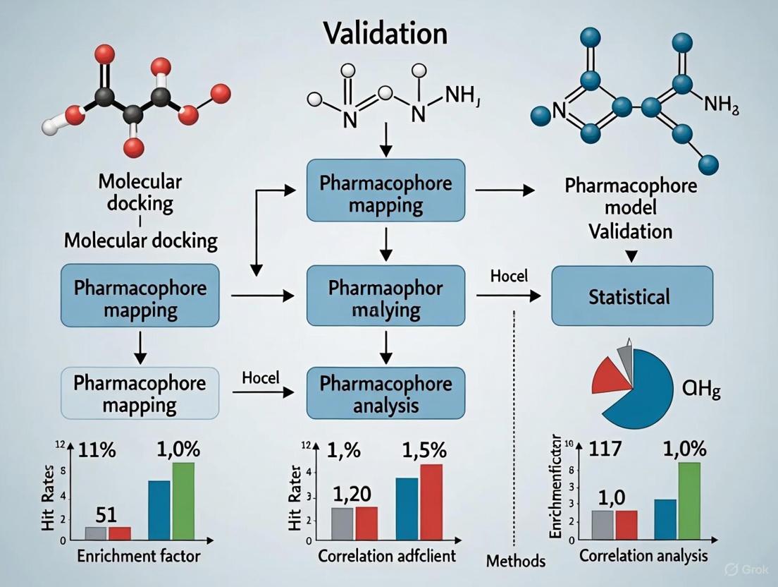
Experimental Workflow Visualization

The following diagram illustrates the logical workflow integrating the various validation methodologies discussed above.

Successful pharmacophore modeling and validation rely on a suite of software tools, databases, and computational resources.

Table 2: Key Research Reagent Solutions for Pharmacophore Validation

Item / Resource	Type	Function in Validation	Example / Source
LigandScout	Software	Used for structure-based and ligand-based pharmacophore generation, model optimization, and decoy set screening [5] [2].	Inte:Ligand
Discovery Studio (DS)	Software	Provides protocols for Ligand Pharmacophore Mapping and validation using the Güner-Henry method [3].	BIOVIA
DUD-E Database	Online Tool	Generates property-matched decoy molecules for rigorous validation of virtual screening performance [1].	https://dude.docking.org/
Protein Data Bank (PDB)	Database	Source of 3D macromolecular structures for structure-based pharmacophore modeling and complex analysis [6] [5].	https://www.rcsb.org/
ZINC/ChEMBL	Database	Curated collections of commercially available compounds and bioactivity data for test set creation and reference [7] [2].	Publicly Accessible
PHASE/Hypogen	Software Algorithm	Implements specific quantitative pharmacophore modeling and validation algorithms, including cost analysis [7].	Schrödinger / BioVia
CATS Descriptors	Computational Method	Chemically Advanced Template Search descriptors used to quantify pharmacophore similarity between molecules [8].	Integrated in various tools

Within modern computational drug discovery, the validation of pharmacophore and Quantitative Structure-Activity Relationship (QSAR) models is paramount. This application note delineates the core statistical metrics—R²pred for external predictive power, RMSE for error magnitude, and Q² for internal robustness via Leave-One-Out (LOO) cross-validation. Framed within best practices for pharmacophore model validation, this document provides researchers and drug development professionals with explicit protocols for calculating and interpreting these metrics, ensuring model reliability, regulatory compliance, and informed decision-making for lead optimization.

The journey from a chemical structure to a predictive computational model hinges on rigorous validation. Without it, models risk being statistical artifacts, incapable of generalizing to new, unseen compounds. Validation provides the critical foundation for trust in model predictions, especially when these predictions influence costly synthetic efforts or regulatory decisions [9] [10].

The OECD principles for QSAR validation underscore the necessity of defining a model's applicability domain and establishing goodness-of-fit, robustness, and predictive power [11]. This document focuses on the quantitative metrics that operationalize these principles. While traditional metrics like the internal Q² and external R²pred are widely used, recent research advocates for supplementary, more stringent parameters like rm² and Rp² to provide a stricter test of model acceptability, particularly in regulatory contexts [9]. This note integrates both traditional and novel metrics to present a comprehensive validation protocol.

Defining the Core Statistical Metrics

R²pred (Predictive R²) for External Validation

Purpose: R²pred is the cornerstone metric for evaluating a model's predictive ability on an external test set of compounds that were not used in model construction [9] [1].

Mathematical Definition: The formula for R²pred is given by: R²pred = 1 - [Σ(Y_observed(test) - Y_predicted(test))² / Σ(Y_observed(test) - Ȳ(training))²] [1].

Here, Y_observed(test) and Y_predicted(test) are the observed and predicted activities of the test set compounds, respectively, and Ȳ(training) is the mean observed activity of the training set compounds.

Interpretation and Acceptance Criterion:

• An R²pred value greater than 0.5 is generally considered to indicate an acceptable and robust model [1].
• A significant advantage of R²pred is that it is independent of the training set's activity range, providing a pure measure of external predictivity [9].

RMSE (Root Mean Square Error)

Purpose: RMSE quantifies the average magnitude of the prediction errors in the units of the biological activity, providing an intuitive measure of model accuracy [1].

Mathematical Definition: RMSE = √[ Σ(Y_observed - Y_predicted)² / n ] [1].

Here, n is the number of compounds. RMSE can be calculated for both the training set (RMSEtr) to assess goodness-of-fit and for the test set (RMSEtest) to assess predictive accuracy.

Interpretation:

• A lower RMSE indicates a more accurate model. There is no universal threshold, as it is highly dependent on the activity range and units. It is most valuable when comparing different models applied to the same dataset.

Q² (LOO Cross-Validated R²) for Internal Validation

Purpose: Q², derived from Leave-One-Out (LOO) cross-validation, assesses the internal robustness and predictive ability of a model within its training set [9] [1].

Methodology: In LOO, one compound is removed from the training set, the model is rebuilt with the remaining compounds, and the activity of the removed compound is predicted. This process is repeated for every compound in the training set.

Mathematical Definition: Q² = 1 - [ Σ(Y_observed(tr) - Y_LOO_predicted(tr))² / Σ(Y_observed(tr) - Ȳ(training))² ] [1].

Interpretation and Acceptance Criterion:

• A Q² > 0.5 is typically considered the threshold for a robust model [12].
• It is crucial to note that a high Q² is a necessary but not sufficient condition for a predictive model; a high Q² does not always guarantee high external predictivity (R²pred) [9].

Table 1: Summary of Core Validation Metrics

Metric	Validation Type	Formula	Interpretation & Acceptance
R²pred	External	1 - [Σ(Y_obs(test) - Y_pred(test))² / Σ(Y_obs(test) - Ȳ_train)²]	> 0.5 indicates acceptable external predictive ability [1].
RMSE	Internal/External	√[ Σ(Y_obs - Y_pred)² / n ]	Lower values indicate higher accuracy; no universal threshold.
Q² (LOO)	Internal	1 - [ Σ(Y_obs(tr) - Y_LOO(tr))² / Σ(Y_obs(tr) - Ȳ_train)² ]	> 0.5 indicates model robustness [12].

Advanced and Supplementary Validation Metrics

While R²pred and Q² are fundamental, relying on them alone can be insufficient. Stricter, novel parameters have been proposed to mitigate the risk of accepting flawed models.

The rm² Metrics: A Stricter Measure

Purpose: The rm² parameter provides a more rigorous assessment by penalizing models for large differences between observed and predicted values [9].

Variants and Calculation:

• rm²(LOO): Applied to the training set using LOO-predicted values.
• rm²(test): Applied to the external test set predictions.
• rm²(overall): A consolidated metric that uses LOO-predicted values for the training set and predicted values for the test set, providing a comprehensive view based on a larger number of compounds [9].

This metric is considered a better and more stringent indicator of predictability than R²pred or Q² alone [9].

Rp² and Randomization Test

Purpose: The Rp² metric is used in conjunction with Y-randomization (Fischer's randomization test) to ensure the model is not the result of a chance correlation [9] [1].

Methodology: The biological activity data is randomly shuffled, and new models are built using the original descriptors. This process is repeated multiple times to generate a distribution of correlation coefficients (Rr) for random models.

Calculation: Rp² penalizes the model's original squared correlation coefficient (R²) for the difference between R² and the squared mean correlation coefficient (Rr²) of the randomized models [9].

A model is considered statistically significant if the original correlation coefficient lies outside the distribution of correlation coefficients from the randomized datasets, confirming the model captures a true structure-activity relationship [1].

Experimental Protocols for Metric Calculation

Protocol 1: Standard External Validation with R²pred and RMSE

Objective: To evaluate the predictive power of a developed QSAR/pharmacophore model on an independent test set.

Materials:

• A validated QSAR/pharmacophore model.
• A curated dataset of compounds with known biological activities, split into training and test sets.

Procedure:

• Data Splitting: Randomly split the full dataset into a training set (typically 70-85%) and a test set (15-30%). Ensure both sets cover a similar range of structural diversity and biological activity [13].
• Model Training: Develop the final model using only the compounds in the training set.
• Prediction: Use the finalized model to predict the biological activities of the compounds in the test set.
• Calculation:
  • Calculate R²pred using the formula in Section 2.1.
  • Calculate RMSE for the test set (RMSEtest) using the formula in Section 2.2.
• Interpretation: A model with R²pred > 0.5 and a low RMSEtest relative to the activity range is considered externally predictive.

Protocol 2: Internal Validation via LOO Cross-Validation for Q²

Objective: To assess the internal robustness and predictive reliability of a model within its training set.

Materials:

• A training set of compounds with known biological activities.

Procedure:

• Model Development: Develop a model using the entire training set (Model A).
• Iterative Prediction:
  • Remove one compound from the training set.
  • Rebuild the model using the remaining N-1 compounds.
  • Predict the activity of the removed compound.
  • Return the removed compound to the training set and repeat the process for every compound in the set.
• Calculation: After all iterations, you will have a LOO-predicted value for every training set compound. Calculate Q² using the formula in Section 2.3.
• Interpretation: A Q² > 0.5 indicates the model is internally robust and stable.

Objective: To perform a stringent, consolidated validation using both internal and external predictions.

Materials:

• A QSAR model, its training set, and an external test set.

Procedure:

• Generate Predictions:
  • Obtain LOO-predicted values for the training set compounds (from Protocol 2).
  • Obtain predicted values for the external test set compounds (from Protocol 1).
• Combine Data: Create a combined dataset of observed vs. predicted values, where predictions for the training set are LOO-based and for the test set are from the final model.
• Calculation: Calculate the rm²(overall) statistic based on this combined dataset [9].
• Interpretation: This metric provides a single, rigorous measure of model predictivity that is less reliant on a potentially small test set and helps in model selection when traditional parameters are comparable.

The following workflow diagrams the integration of these validation protocols into a coherent model development process:

The Scientist's Toolkit: Essential Reagents & Software

Table 2: Key Research Reagents and Computational Tools for Model Validation

Item/Software	Function/Description	Example Use in Validation
Cerius2, DRAGON	Software for calculating molecular descriptors (topological, structural, physicochemical) [9] [14].	Generates independent variables for QSAR model development.
Schrödinger Suite	Integrated software for drug discovery, including LigandScout (pharmacophore) and Phase (3D-QSAR) [15] [16].	Used for pharmacophore generation, model building, and performing LOO validation.
V-Life MDS	A software platform for molecular modeling and QSAR studies [17].	Calculates 2D and 3D molecular descriptors and builds QSAR models with internal validation.
Decoy Set (from DUD-E)	A database of physically similar but chemically distinct inactive molecules used for validation [1] [15].	Validates the pharmacophore model's ability to distinguish active from inactive compounds (enrichment assessment).
Test Set Compounds	A carefully selected, independent set of compounds not used in model training.	Serves as the benchmark for calculating R²pred and RMSEtest for external validation [1].

A robust validation strategy is non-negotiable for any pharmacophore or QSAR model intended for reliable application in drug discovery. While the classical triumvirate of Q², R²pred, and RMSE provides a foundational assessment, researchers are strongly encouraged to adopt a more comprehensive approach. Incorporating stringent metrics like rm² and Rp² offers a deeper, more reliable evaluation of model performance, aligning with the best practices for regulatory acceptance and effective lead optimization as outlined in this note. A model that successfully passes this multi-faceted validation protocol provides a trustworthy foundation for virtual screening and the rational design of novel therapeutic agents.

In the rigorous field of computer-aided drug design, the predictive power of a pharmacophore model is paramount. A pharmacophore model abstractly represents the ensemble of steric and electronic features necessary for a molecule to interact with a biological target and elicit a response [6]. However, not all generated models are created equal; some may fit the training data by mere chance rather than capturing a true underlying structure-activity relationship. Cost function analysis provides a critical, quantitative framework to ascertain the robustness and statistical significance of a pharmacophore hypothesis [1]. It is a cornerstone of model validation, ensuring that the model possesses genuine predictive capability and is not a product of overfitting or random correlation. Within this analytical framework, two specific cost parameters—the null hypothesis cost and the configuration cost—serve as fundamental indicators of model quality and reliability. This application note details the interpretation of these costs and provides a validated protocol for their use within pharmacophore model validation workflows.

Deciphering Cost Function Components

The total cost of a pharmacophore hypothesis is a composite value calculated during the model generation process, such as by the HypoGen algorithm [18]. It integrates several cost components, each providing unique insight into the model's quality. A comprehensive breakdown of these components is provided in the table below.

Table 1: Key Components of Pharmacophore Cost Function Analysis

Cost Component	Description	Interpretation & Ideal Value
Total Cost	The overall cost of the developed pharmacophore hypothesis.	Should be as low as possible.
Fixed Cost	The ideal cost of a hypothetical "perfect" model that fits all data perfectly [19].	A theoretical lower bound. The total cost should be close to this value.
Null Hypothesis Cost	The cost of a model that assumes no relationship between features and activity (i.e., the mean activity of all training set compounds is used for prediction) [1] [19].	A baseline for comparison. A large difference from the total cost indicates a significant model.
Configuration Cost	A fixed cost that depends on the complexity of the hypothesis space, influenced by the number of features in the model [1].	Should generally be < 17 [1]. A higher value suggests an overly complex model.
Weight Cost	Penalizes models where the feature weights deviate from the ideal value [1].	Lower values indicate a more ideal configuration.
Error Cost	Represents the discrepancy between the predicted and experimentally observed activities of the training set compounds [1].	A major driver of the total cost; lower values indicate better predictive accuracy.

Interpreting the Null Hypothesis Cost and ΔCost

The null hypothesis cost represents the starting point of the analysis, calculating the cost of a model that has no correlation with biological activity [19]. The most critical metric derived from this is the ΔCost (cost difference), calculated as: ΔCost = Null Cost - Total Cost [19].

The ΔCost value is a direct indicator of the statistical significance of the pharmacophore model. A larger ΔCost signifies that the developed hypothesis is far from a random chance correlation. As established in validated protocols, a ΔCost of more than 60 implies that the hypothesis does not merely reflect a chance correlation and has a greater than 90% probability of representing a true correlation [1] [19]. Models with a ΔCost below this threshold should be treated with caution.

Understanding Configuration Cost

The configuration cost is a fixed value that increases with the complexity of the hypothesis space, which is directly related to the number of features used in the pharmacophore model [1]. It represents a penalty for model complexity, discouraging the creation of overly specific models that may not generalize well.

A configuration cost below 17 is considered satisfactory for a robust pharmacophore model [1]. A high configuration cost suggests that the model is too complex and may be over-fitted to the training set, reducing its utility for predicting the activity of new, diverse compounds. Therefore, the goal is to find a model with a high ΔCost while maintaining a low configuration cost.

The following diagram illustrates the logical relationship between these key cost components and the decision process for model acceptance.

Experimental Protocol for Cost Analysis in Model Validation

This protocol provides a step-by-step methodology for performing cost function analysis during the generation and validation of a 3D QSAR pharmacophore model, using software such as Accelrys Discovery Studio's HypoGen.

Materials and Software Requirements

Table 2: Research Reagent Solutions for Pharmacophore Modeling & Cost Analysis

Item Name	Function / Description	Example Tools / Sources
Chemical Dataset	A curated set of compounds with known biological activities (e.g., IC50, Ki) and diverse chemical structures.	ChEMBL, PubChem BioAssay [7]
Molecular Modeling Suite	Software for compound sketching, 3D structure generation, energy minimization, and conformational analysis.	ChemSketch, ChemBioOffice [20] [18]
Pharmacophore Modeling Software	Platform capable of generating 3D QSAR pharmacophore hypotheses and performing cost function analysis.	Accelrys Discovery Studio (HypoGen) [19] [18], Catalyst (Hypogen) [7], LigandScout [21]
Conformation Generation Algorithm	Generates a representative set of low-energy 3D conformers for each compound in the dataset.	Poling Algorithm, CHARMm force field [22] [18]

Step-by-Step Procedure

• Training Set Preparation

  • Select a set of compounds (typically 15-25 molecules) with known biological activities spanning a wide range (e.g., 4-5 orders of magnitude) [18].
  • Sketch the 2D structures of the training set compounds and convert them into 3D models.
  • Generate multiple low-energy conformations for each compound to represent its flexibility. A common setting is a maximum of 255 conformations within an energy threshold of 20 kcal/mol above the global minimum [20] [18].

• Pharmacophore Generation and Cost Calculation

  • Input the training set conformations and their experimental activity values into the pharmacophore generation module (e.g., HypoGen).
  • Run the hypothesis generation process. The algorithm will typically output the top 10 ranked models.
  • From the results, extract the following cost values for each hypothesis: Total Cost, Fixed Cost, Null Cost, and Configuration Cost.

• Cost Analysis and Model Selection

  • For each hypothesis, calculate the ΔCost (Null Cost - Total Cost).
  • Apply the significance criteria:
    • Primary Filter: Retain only models with a ΔCost > 60 [1] [19].
    • Complexity Filter: From the shortlisted models, prioritize those with a Configuration Cost < 17 [1].
  • The model with the highest ΔCost and a low Configuration Cost should be selected as the best, statistically significant pharmacophore hypothesis.

Validation and Integration with Other Methods

While cost function analysis is a powerful internal validation tool, a comprehensive validation strategy for a pharmacophore model requires its integration with other methods.

• Test Set Prediction: Use an external test set of compounds (not used in training) to evaluate the model's predictive power. Calculate metrics like the predictive correlation coefficient (R²pred) and root-mean-square error (RMSE). An R²pred greater than 0.50 is often considered acceptable [1].
• Fischer Randomization Test: This test assesses the risk of chance correlation. The activities of the training set are randomly shuffled, and new models are generated from this scrambled data. The original model's cost should be significantly lower than the costs from hundreds of randomized iterations, confirming its statistical significance [1] [20] [18].
• Decoy Set Validation: Evaluate the model's ability to discriminate active compounds from inactive ones (decoys) in a database. Metrics like the Enrichment Factor (EF) and Goodness of Hit Score (GH) are used, where a GH score above 0.7 indicates a very good model [1] [20].

Application Notes and Troubleshooting

• Low ΔCost (< 60): This indicates a model that is likely not statistically significant. To address this, re-examine the training set for diversity and a sufficient spread of activity values. Ensure conformational sampling is adequate.
• High Configuration Cost (≥ 17): This suggests an overly complex model. Try generating models with a smaller number of pharmacophoric features.
• Holistic Evaluation: Always interpret cost values in conjunction with other statistical parameters (like correlation coefficient) and validation results from test sets and Fischer randomization. A model with excellent cost parameters but poor predictive performance on a test set should not be trusted.

Cost function analysis, particularly the interpretation of the null hypothesis cost and configuration cost, provides an indispensable foundation for robust pharmacophore model validation. A ΔCost > 60 signifies a model unlikely to be a product of chance, while a configuration cost < 17 guards against overfitting. By adhering to this protocol and integrating it with other validation techniques such as Fischer randomization and decoy set validation, researchers can confidently select pharmacophore models with genuine predictive power. This rigorous approach significantly enhances the efficiency of virtual screening and the likelihood of successfully identifying novel lead compounds in drug discovery campaigns.

In pharmacophore model validation, the robustness of the test set—defined by its chemical diversity and structural variety—is a critical determinant of predictive accuracy and real-world applicability. Pharmacophore models abstract the essential steric and electronic features necessary for a ligand to interact with a biological target, forming the foundation for virtual screening in computer-aided drug design [6] [23]. However, even a perfectly conceived pharmacophore hypothesis remains functionally unvalidated without rigorous testing against a representative set of compounds that adequately captures the chemical space of interest.

A robust test set serves as the ultimate proving ground, challenging the pharmacophore model's ability to generalize beyond the training compounds and correctly identify structurally diverse active molecules while rejecting inactive ones. The composition of this test set directly impacts validation metrics such as enrichment factors and Güner-Henry scores, which measure the model's practical utility in drug discovery campaigns [3] [24]. Without careful attention to chemical diversity and structural variety, researchers risk developing models that perform well on paper but fail to identify novel scaffolds in virtual screening experiments, ultimately wasting valuable resources on false leads.

The critical importance of test set design stems from the fundamental challenges in chemoinformatics. Models derived from limited chemical space tend to exhibit poor extrapolation capabilities when confronted with structurally diverse compounds or those containing unusual functional groups [25]. Furthermore, the presence of structural outliers—compounds with unique moieties not represented in the training data—can disproportionately influence model performance if not properly accounted for in the test set [25]. Therefore, a strategically designed test set acts as a diagnostic tool, revealing potential weaknesses and ensuring the model's stability against the natural variations found in large chemical databases.

Theoretical Foundation: Why Test Set Composition Matters

The Relationship Between Chemical Space and Model Generalization

The concept of chemical space represents a fundamental framework for understanding model generalization in pharmacophore-based virtual screening. Chemical space encompasses all possible molecules and their associated properties, forming a multidimensional continuum where compounds with similar structural features and biological activities tend to cluster [25] [26]. A robust pharmacophore model must effectively navigate this space to identify novel active compounds, making comprehensive test set coverage essential for meaningful validation.

Pharmacophore models developed without adequate consideration of chemical space coverage often suffer from overfitting to the training compounds' specific structural patterns. Such models may demonstrate excellent performance for compounds similar to those in the training set but fail to identify active compounds with different scaffolds or substitution patterns [25]. This limitation directly impacts virtual screening efficiency, as evidenced by studies showing that stepwise and adaptive selection approaches with better chemical space coverage yield models with superior error performance and stability compared to traditional methods [25].

The Impact of Structural Outliers and Domain of Applicability

Structural outliers—compounds characterized by unique chemical groups or structural motifs not well-represented in the training data—present a particular challenge for pharmacophore models [25]. These compounds often reside in sparsely populated regions of the chemical space and can significantly influence model performance if not properly accounted for during validation. A test set lacking such structural diversity provides a false sense of security by not challenging the model's boundaries of applicability.

The domain of applicability defines the chemical space region where a model's predictions can be considered reliable. A well-constructed test set should systematically probe this domain by including compounds at the periphery of the chemical space, not just those near the densely populated core regions [25]. Research has shown that the property of a molecule to be a structural outlier can depend on the descriptor set used, further emphasizing the need for test sets that challenge the model from multiple representational perspectives [25].

Table 1: Types of Chemical Diversity in Robust Test Sets

Diversity Dimension	Description	Impact on Model Validation
Scaffold Diversity	Variation in core molecular frameworks	Tests model's ability to recognize actives beyond training scaffolds
Functional Group Diversity	Inclusion of different chemical moieties	Challenges feature identification and alignment
Property Diversity	Range of molecular weight, logP, etc.	Ensures model works across property space
Complexity Diversity	Variation in molecular size and complexity	Tests feature selection and weighting

Protocols for Constructing Robust Test Sets

Experimental Protocol: Systematic Test Set Construction with Chemical Diversity Analysis

Objective: To construct a test set with sufficient chemical diversity and structural variety to rigorously validate pharmacophore model performance and generalization capability.

Materials and Reagents:

• Compound databases (e.g., ZINC, ChEMBL, commercial collections)
• Chemical structure visualization software (e.g., ChemBioOffice)
• Computational chemistry tools (e.g., Discovery Studio, Schrödinger Suite)
• Diversity analysis scripts or software (e.g., RDKit, Canvas)

Procedure:

• Define the Chemical Space Boundaries

  • Compile all available active compounds for the target of interest from public databases (e.g., ChEMBL, BindingDB) and literature sources [24] [2]
  • Calculate molecular descriptors (e.g., molecular weight, logP, topological polar surface area, hydrogen bond donors/acceptors) to characterize the property space
  • Perform principal component analysis (PCA) on the descriptor matrix to identify the major dimensions of variation within the active compounds [25]

• Select Structurally Diverse Actives

  • Apply maximum dissimilarity selection algorithms (e.g., Kennard-Stone) to identify compounds that span the chemical space defined in step 1 [25]
  • Ensure representation of different molecular scaffolds, not just varying side chains
  • Include compounds with unusual structural features or functional groups that may challenge the pharmacophore model
  • Verify that the selected compounds cover the range of bioactivity values (e.g., IC50, Ki) relevant to the project goals

• Curate Decoy Compounds with Matched Properties

  • Generate decoy compounds using tools such as the Database of Useful Decoys (DUDe) or similar approaches [2]
  • Match decoys to active compounds based on molecular weight, logP, and other physicochemical properties but ensure topological dissimilarity
  • Include decoys with similar functional groups but different spatial arrangements to test the model's geometric specificity
  • Apply drug-like filters (e.g., Lipinski's Rule of Five) if relevant to the project's therapeutic context [24]

• Validate Test Set Diversity

  • Calculate pairwise molecular similarity metrics (e.g., Tanimoto coefficients) to verify structural diversity [25]
  • Visualize the chemical space coverage using dimensionality reduction techniques (t-SNE, UMAP) to confirm that the test set adequately represents the applicable chemical space [26]
  • Ensure the test set includes compounds that probe specific pharmacophore features (e.g., hydrogen bond donors/acceptors, hydrophobic regions, charged groups)

Experimental Protocol: Statistical Validation of Test Set Composition

Objective: To quantitatively assess the chemical diversity and structural variety of a test set using statistical measures and ensure its suitability for pharmacophore model validation.

Materials and Reagents:

• Pre-constructed test set (from Protocol 3.1)
• Statistical analysis software (e.g., R, Python with pandas, scikit-learn)
• Molecular fingerprint generation tools (e.g., RDKit, OpenBabel)
• Diversity metrics calculation scripts

Procedure:

• Calculate Diversity Metrics

  • Generate molecular fingerprints (e.g., ECFP4, FCFP6) for all test set compounds
  • Compute pairwise Tanimoto similarity matrix and analyze the distribution
  • Calculate internal diversity metrics: mean pairwise similarity, similarity percentile ranges
  • Determine scaffold diversity using Bemis-Murcko framework analysis and count unique scaffolds

• Assess Chemical Space Coverage

  • Perform PCA on the fingerprint descriptor space and project training and test sets
  • Calculate the coverage ratio: percentage of training set chemical space covered by the test set
  • Identify coverage gaps where the test set lacks representatives from certain regions of the training set chemical space
  • Use Euclidean distance histograms in the latent feature space to quantify diversity as demonstrated in MAD dataset analyses [26]

• Evaluate Activity Distribution

  • Ensure the test set covers the full range of bioactivity values present in the available data
  • Verify that the distribution of active versus inactive compounds reflects realistic screening expectations (typically 0.1-1% actives for enrichment calculations)
  • Stratify the test set by activity class (high, medium, low, inactive) and verify diversity within each stratum

• Perform Cluster Analysis

  • Apply clustering algorithms (e.g., k-means, hierarchical clustering) to the chemical descriptor space
  • Verify that test set compounds represent multiple clusters rather than concentrating in a few chemical classes
  • Ensure that each major cluster contains both active and inactive compounds to test the model's discriminative power within chemical neighborhoods

Table 2: Key Statistical Metrics for Test Set Evaluation

Metric Category	Specific Metrics	Target Values	Interpretation
Structural Diversity	Mean pairwise Tanimoto similarity, Unique scaffolds/Total compounds	<0.5 similarity, >30% unique scaffolds	Lower similarity and higher scaffold count indicate greater diversity
Chemical Space Coverage	Percentage of training set PCA space covered, Gap analysis	>80% coverage, Minimal large gaps	Higher coverage ensures comprehensive testing of model applicability
Activity Representation	Range of pIC50/pKi values, Active/inactive ratio	Full range, 0.1-1% actives	Complete activity range tests predictive accuracy across potencies
Cluster Distribution	Number of clusters represented, Balance across clusters	Multiple clusters, Reasonable balance	Ensures testing across different chemical classes

Validation Methods for Assessing Pharmacophore Model Performance

Experimental Protocol: Güner-Henry (GH) Validation Method

Objective: To validate pharmacophore model performance using the Güner-Henry method, which measures the model's ability to enrich active compounds from a test set containing both active and decoy molecules.

Materials and Reagents:

• Validated pharmacophore model (structure-based or ligand-based)
• Test set with known active compounds and decoys
• Virtual screening software (e.g., Discovery Studio, LigandScout)
• Calculation spreadsheet for GH metrics

Procedure:

• Prepare the Test Database

  • Combine known active compounds (A) with decoy compounds (D) to create a test database of size N
  • Ensure the total number of actives (A) is known and the decoys are property-matched but chemically distinct
  • For the test set, typical sizes range from 1,000 to 10,000 compounds with active compound percentages between 0.1% and 1% [3] [2]

• Perform Pharmacophore-Based Screening

  • Screen the entire test database against the pharmacophore model using flexible search methods
  • Record the number of hits (Ht) obtained from the screening process
  • From the hits, identify how many are true actives (Ha)

• Calculate Güner-Henry Metrics

  • Compute the enrichment factor (EF) using the formula: EF = (Ha/Ht) / (A/N)
  • Calculate the GH score using the comprehensive formula that incorporates yield of actives and false positives
  • Determine the percentage yield of actives: (Ha/Ht) × 100
  • Calculate the percentage ratio of actives: (Ha/A) × 100 [3]

• Interpret the Results

  • Compare the EF value to ideal enrichment: EF = 1 indicates random performance, while higher values indicate better enrichment
  • Evaluate the GH score on a scale of 0-1, where values closer to 1 indicate better model performance
  • Assess the balance between sensitivity (Ha/A) and specificity (1 - false positive rate) based on the results

Experimental Protocol: Receiver Operating Characteristic (ROC) Analysis

Objective: To evaluate the discriminative power of a pharmacophore model using ROC analysis, which provides a comprehensive view of the model's sensitivity and specificity across all classification thresholds.

Materials and Reagents:

• Pharmacophore model with scoring function
• Test set with known active and inactive compounds
• Statistical analysis software with ROC curve capabilities
• Spreadsheet software for data recording and visualization

Procedure:

• Generate Pharmacophore Fit Scores

  • Screen all test set compounds (both active and inactive) against the pharmacophore model
  • Record the fit score or alignment score for each compound
  • For multi-conformer compounds, use the best-fitting conformation

• Calculate Sensitivity and Specificity Across Thresholds

  • Sort compounds by their fit scores in descending order
  • Systematically vary the classification threshold from the highest to lowest fit score
  • At each threshold, calculate:
    • True Positives (TP): Active compounds with fit score ≥ threshold
    • False Positives (FP): Inactive compounds with fit score ≥ threshold
    • True Negatives (TN): Inactive compounds with fit score < threshold
    • False Negatives (FN): Active compounds with fit score < threshold
  • Compute sensitivity (Recall) = TP/(TP+FN)
  • Compute specificity = TN/(TN+FP)
  • Compute 1 - Specificity (False Positive Rate)

• Generate and Interpret ROC Curve

  • Plot the ROC curve with False Positive Rate (1-Specificity) on the x-axis and Sensitivity on the y-axis
  • Calculate the Area Under the Curve (AUC) using numerical integration methods
  • Interpret the AUC value:
    • AUC = 0.5: No discriminative power (random classification)
    • 0.7 ≤ AUC < 0.8: Acceptable discriminative power
    • 0.8 ≤ AUC < 0.9: Excellent discriminative power
    • AUC ≥ 0.9: Outstanding discriminative power [2]

• Calculate Additional Performance Metrics

  • Compute Precision = TP/(TP+FP)
  • Calculate F1-Score = 2 × (Precision × Recall)/(Precision + Recall)
  • Determine Optimal Threshold using Youden's J statistic (Sensitivity + Specificity - 1)

Case Studies and Applications

Case Study: XIAP Inhibitor Discovery with Validated Test Sets

In a comprehensive study targeting X-linked inhibitor of apoptosis protein (XIAP) for cancer therapy, researchers demonstrated the critical importance of robust test sets in pharmacophore validation [2]. The study employed a structure-based pharmacophore model generated from a protein-ligand complex (PDB: 5OQW) containing a known inhibitor with experimentally measured IC50 value of 40.0 nM.

Test Set Design and Validation:

• The test set comprised 10 known XIAP antagonists with experimentally determined IC50 values merged with 5,199 decoy compounds obtained from the Directory of Useful Decoys (DUDe)
• This carefully designed test set with a high ratio of decoys to actives (approximately 520:1) provided a rigorous challenge for the pharmacophore model
• The chemical diversity of the test set was ensured by including compounds with varied scaffolds and functional groups, effectively representing the chemical space of potential XIAP binders

Validation Results:

• The pharmacophore model achieved an exceptional early enrichment factor (EF1%) of 10.0, indicating strong ability to identify active compounds in the early stages of virtual screening
• The area under the ROC curve (AUC) value reached 0.98 at the 1% threshold, demonstrating outstanding discriminative power between active and decoy compounds
• This high-level performance was directly attributable to the comprehensive test set that thoroughly probed the model's capabilities across diverse chemical structures

Virtual Screening Outcome:

• Subsequent virtual screening of natural product databases identified seven hit compounds, with three (Caucasicoside A, Polygalaxanthone III, and MCULE-9896837409) showing particular promise in molecular dynamics simulations
• The success in identifying novel natural product scaffolds with potential XIAP inhibitory activity underscored the value of rigorous test set validation in practical drug discovery applications

Case Study: Akt2 Inhibitor Development with Dual Pharmacophore Approach

A study focused on discovering novel Akt2 inhibitors for cancer therapy implemented a dual pharmacophore approach validated with comprehensive test sets [24]. The researchers developed both structure-based and 3D-QSAR pharmacophore models, then applied stringent validation protocols to ensure their utility in virtual screening.

Test Set Composition:

• The test set for the structure-based pharmacophore included 63 known active compounds collected from scientific literature, spanning a range of bioactivities
• For the 3D-QSAR pharmacophore, a separate test set of 40 molecules was used to validate the model's predictive accuracy
• Decoy set validation employed 2,000 molecules consisting of 1,980 compounds with unknown activity and 20 known Akt2 inhibitors

Test Set Diversity Considerations:

• The test sets included compounds with different molecular scaffolds to challenge the models' ability to recognize essential pharmacophore features across diverse chemical contexts
• Activity values spanned multiple orders of magnitude, ensuring the models could distinguish not just actives from inactives but also highly potent from moderately active compounds
• The high proportion of decoys in the validation set (99% of the total) created a realistic simulation of virtual screening conditions where active compounds are rare

Validation Outcomes:

• The structure-based pharmacophore model (PharA) contained seven pharmacophoric features and successfully identified active compounds that mapped to at least six of these features
• Both models demonstrated strong performance in test set and decoy set validation, giving confidence to proceed with virtual screening of large compound databases
• The subsequent screening of nearly 700,000 compounds from natural product and commercial databases, followed by drug-like filtering and ADMET analysis, identified seven promising hit compounds with diverse scaffolds

Table 3: Essential Research Reagents and Tools for Test Set Construction and Validation

Reagent/Tool Category	Specific Examples	Primary Function	Application Context
Compound Databases	ZINC, ChEMBL, BindingDB, Coconut Database	Source of active and diverse compounds for test sets	Provides chemical structures and bioactivity data for test set construction [24] [2] [27]
Decoy Generation Tools	DUDe (Directory of Useful Decoys)	Generate property-matched but topologically distinct inactive compounds	Creates challenging negative controls for validation [2]
Diversity Analysis Software	RDKit, Canvas, Schrodinger Suite	Calculate molecular similarity, clustering, and diversity metrics	Quantifies test set diversity and chemical space coverage [25]
Virtual Screening Platforms	Discovery Studio, LigandScout, Phase	Perform pharmacophore-based screening and fit score calculation	Generates hit lists and scores for validation metrics [28] [24] [2]
Validation Metric Calculators	Custom scripts for GH scoring, ROC analysis	Compute enrichment factors, AUC values, and other validation parameters	Quantitatively assesses model performance [3] [24]

The critical importance of robust test sets in pharmacophore model validation cannot be overstated. As demonstrated throughout this protocol, test sets characterized by extensive chemical diversity and structural variety serve as the essential proving ground for pharmacophore models, challenging their ability to generalize beyond training compounds and perform effectively in real-world virtual screening applications. The comprehensive protocols outlined for test set construction, statistical validation, and performance assessment provide researchers with practical methodologies to ensure their pharmacophore models are rigorously evaluated before deployment in resource-intensive drug discovery campaigns.

The case studies examining XIAP and Akt2 inhibitor discovery underscore how thoughtfully constructed test sets directly contribute to successful identification of novel lead compounds [24] [2]. By implementing the Güner-Henry method, ROC analysis, and chemical diversity assessments detailed in these application notes, researchers can significantly increase confidence in their pharmacophore models and improve the efficiency of subsequent virtual screening efforts. In an era where computational approaches play an increasingly central role in drug discovery, robust validation practices centered on chemically diverse test sets remain fundamental to translating in silico predictions into biologically active therapeutic agents.

The Validation Toolkit: Step-by-Step Protocols for Assessing Model Performance

The rigorous validation of computational models is a cornerstone of credible research in computer-aided drug design (CADD). Pharmacophore models, which abstract the essential steric and electronic features required for molecular recognition, are powerful tools for virtual screening [6] [29]. However, their predictive performance can be misleading if evaluated using biased benchmark datasets. The Decoy Set Method addresses this critical issue by employing carefully selected, non-binding molecules (decoys) to simulate a realistic screening scenario and provide an unbiased estimate of model effectiveness [30]. This Application Note details the implementation of this method using the DUD-E (Database of Useful Decoys: Enhanced) benchmark, providing a structured protocol for the rigorous evaluation of pharmacophore models within a best-practice framework for validation methods research [30] [31].

The DUD-E Database: A Foundation for Unbiased Benchmarking

DUD-E is a widely adopted benchmark database designed to eliminate the artificial enrichment that plagued earlier benchmarking sets. Its development was driven by the need for a rigorous and realistic platform for evaluating structure-based virtual screening (SBVS) methods [30] [31].

Core Principles and Design

The fundamental principle of DUD-E is to provide decoy molecules that are physically similar yet chemically distinct from known active molecules for a given target. This "property-matched decoy" strategy is engineered to minimize biases that could allow trivial discrimination based on simple physicochemical properties alone [30]. The design of DUD-E incorporates several key aspects:

• Physicochemical Matching: Decoys are matched to actives based on key properties such as molecular weight, calculated logP, and number of hydrogen bond donors and acceptors. This ensures that simple property-based filters cannot easily separate actives from decoys [30].
• Chemical Dissimilarity: Despite physical similarity, decoys are chemically distinct from actives to ensure they are unlikely to bind the target. This is typically assessed via topological fingerprinting, ensuring decoys do not share key functional motifs with actives [30].
• Drug-like Nature: Decoys are sourced from databases like ZINC and are selected to exhibit drug-like properties, making the virtual screening experiment more representative of a real-world drug discovery campaign [30].

The table below summarizes the quantitative scope of the DUD-E database, highlighting its extensive coverage of targets and compounds, which provides a robust foundation for statistical evaluation.

Table 1: Quantitative Summary of the DUD-E Database Scope

Category	Description	Value
Target Coverage	Number of protein targets included	102 targets [30]
Ligand Coverage	Number of active ligands	~22,000 active compounds [30]
Decoy Ratio	Average number of decoys per active	50 decoys per active [30]
Key Property	Reported average DOE score of original DUD-E decoys	0.166 [30]

Quantitative Evaluation Metrics and Protocol

A rigorous evaluation requires a set of quantitative metrics to assess the performance of a pharmacophore model in distinguishing actives from decoys. The following section outlines the key metrics and a standardized protocol for their calculation.

Key Performance Metrics

The performance of a virtual screening method is typically evaluated using enrichment-based metrics and statistical measures derived from the ranking of actives and decoys.

Table 2: Key Quantitative Metrics for Pharmacophore Model Evaluation

Metric	Formula/Description	Interpretation
AUC ROC	Area Under the Receiver Operating Characteristic curve	Measures the overall ability to rank actives above decoys. A value of 0.5 indicates random performance, 1.0 indicates perfect separation [30].
Enrichment Factor (EF)	(Hitssselected / Nselected) / (Hitsstotal / Ntotal)	Measures the concentration of actives in a selected top fraction of the screened database compared to a random selection [29].
Recall (True Positive Rate)	TP / (TP + FN)	The fraction of all known actives that were successfully retrieved by the model [32].
Precision	TP / (TP + FP)	The fraction of retrieved compounds that are actually active [32].
DOE Score	Deviation from Optimal Embedding; a measure of physicochemical property matching between actives and decoys.	A lower score indicates superior property matching, reducing the risk of artificial enrichment. DeepCoy improved the average DUD-E DOE from 0.166 to 0.032 [30].

Experimental Validation Protocol

This protocol provides a step-by-step guide for using DUD-E to evaluate a pharmacophore model.

1. Data Acquisition and Preparation:

• Download the DUD-E dataset for your target of interest from the official website (http://dude.docking.org/).
• Prepare the ligand files (both actives and decoys) for screening. This typically involves:
  • Format Conversion: Ensure all structures are in a consistent format (e.g., SDF, MOL2).
  • Tautomer and Stereoisomer Enumeration: Generate possible tautomers and stereoisomers for molecules with undefined chiral centers or double bonds [32].
  • Conformer Generation: For flexible molecules, generate a representative ensemble of 3D conformations. A common practice is to generate up to 100 conformers per molecule within a defined energy range (e.g., 50 kcal/mol) using a force field like MMFF94 [32].

2. Pharmacophore-Based Virtual Screening:

• Load your pharmacophore model into a suitable software platform (e.g., LigandScout [29]).
• Screen the prepared database of actives and decoys against the model.
• The screening process often involves multiple steps to enhance efficiency [32]:
  • Fingerprint Pre-screening: Use pharmacophore fingerprints as a Bloom filter to quickly discard molecules that are highly unlikely to match.
  • Geometric Mapping: For the remaining candidates, perform a subgraph isomorphism check to see if the pharmacophore's topology is present.
  • 3D Hash Comparison: Finally, compare the 3D pharmacophore hashes of the query model and the candidate molecules to confirm a match with identical topology and stereoconfiguration.

3. Result Analysis and Metric Calculation:

• Ranking: Rank all screened compounds (actives and decoys) based on the pharmacophore fit value or scoring function.
• Calculate Metrics: Using the ranked list, calculate the performance metrics outlined in Table 2, such as AUC ROC, EF at 1% and 10%, and precision-recall curves.
• Visual Inspection: Manually inspect the top-ranked hits to validate the proposed binding mode and the rationale behind the model's selections.

Advanced Application: Generating Improved Decoys with DeepCoy

While DUD-E provides a robust baseline, recent advances in deep learning offer methods to generate even more rigorously matched decoys, further reducing potential bias.

The DeepCoy Methodology

DeepCoy is a deep learning-based approach that frames decoy generation as a multimodal graph-to-graph translation problem [30]. It uses a variational autoencoder framework with graph neural networks to generate decoys from active molecules.

Workflow Overview:

• Input: An active molecule is provided as a graph.
• Encoding: The graph is encoded into a latent representation.
• Decoding: A new molecular graph (the decoy) is generated from this representation in a "bond-by-bond" manner, guided by chemical valency rules [30].
• Output: The generated decoy matches the physicochemical properties of the input active but is structurally dissimilar, minimizing the risk of being a false negative [30].

Quantitative Performance of DeepCoy

The table below compares the performance of DeepCoy-generated decoys against the original DUD-E decoys, demonstrating a significant reduction in bias.

Table 3: Quantitative Comparison of DeepCoy vs. Original DUD-E Decoys

Metric	Original DUD-E Decoys	DeepCoy-Generated Decoys	Improvement
Average DOE Score	0.166 [30]	0.032 [30]	81% decrease
Virtual Screening AUC (Autodock Vina)	0.70 [30]	0.63 [30]	Performance closer to random, indicating harder-to-distinguish decoys

The Research Toolkit

A successful evaluation requires a suite of software tools and data resources. The following table catalogues essential reagents for implementing the DUD-E decoy set method.

Table 4: Essential Research Reagents and Software Solutions

Item Name	Type	Function in Protocol	Access Information
DUD-E Database	Data Resource	Provides the benchmark set of active and property-matched decoy molecules for rigorous validation.	http://dude.docking.org/ [30]
DeepCoy	Software Tool	Generates deep learning-improved decoys with tighter property matching to actives, further reducing dataset bias.	https://github.com/oxpig/DeepCoy [30]
LigandScout	Software Tool	A comprehensive platform for structure- and ligand-based pharmacophore model creation, refinement, and virtual screening.	Commercial & Academic Licenses [29]
ROCS	Software Tool	Performs rapid shape and "color" (chemical feature) overlay of molecules, useful for scaffold hopping and validation.	Commercial (OpenEye) [31]
PLANTS	Software Tool	A molecular docking software used for flexible ligand sampling; can be integrated with pharmacophore constraints.	Academic Free License [31]
RDKit	Software Tool	An open-source cheminformatics toolkit used for fundamental tasks like conformer generation, fingerprinting, and molecule manipulation.	Open Source [32]

Workflow Visualization

The following diagram illustrates the complete experimental workflow for the rigorous evaluation of a pharmacophore model using the DUD-E framework, from data preparation to final performance assessment.

Workflow for Pharmacophore Model Evaluation Using DUD-E

The implementation of the decoy set method using the DUD-E database represents a best practice in pharmacophore model validation. By providing a large set of property-matched decoys, DUD-E mitigates the risk of artificial enrichment and ensures that reported performance metrics reflect a model's true capacity for molecular recognition rather than its ability to exploit dataset biases. The integration of advanced tools like DeepCoy can further refine this process, generating decoys that push the boundaries of rigorous benchmarking. Adherence to the detailed protocols and quantitative evaluation frameworks outlined in this Application Note will empower researchers to deliver robust, reliable, and scientifically credible pharmacophore models, thereby strengthening the foundation of computer-aided drug discovery.

Fischer's Randomization Test is a cornerstone statistical method in pharmacophore model validation, serving as a critical safeguard against chance correlations. This protocol details the systematic application of the test within the drug discovery pipeline, providing researchers with a robust framework to distinguish meaningful structure-activity relationships from random artifacts. By implementing this methodology, scientists can enhance the predictive reliability of their pharmacophore models before proceeding to resource-intensive virtual screening and experimental validation stages.

In computational drug discovery, pharmacophore models abstract the essential steric and electronic features necessary for molecular recognition by a biological target. However, any quantitative model derived from a limited set of compounds risks capturing accidental correlations rather than genuine biological relationships. Fischer's Randomization Test (also referred to as a permutation test) addresses this fundamental validation challenge by providing a statistical framework to quantify the probability that the observed correlation occurred by random chance [1].

The test operates on a straightforward premise: if the original pharmacophore model captures a true structure-activity relationship, then randomizing the biological activity values across the training set compounds should rarely produce hypotheses with comparable or better statistical significance. By repeatedly generating pharmacophore models from these randomized datasets, researchers can construct a distribution of correlation coefficients under the null hypothesis of no true relationship, then determine where the original model's correlation falls within this distribution [1] [24]. This approach has become a standard validation component across diverse drug discovery applications, including histone deacetylase [33], Akt2 [24], and butyrylcholinesterase inhibitors [34].

Theoretical Foundation and Statistical Principles

Historical Context and Development

The randomization test was initially developed by Ronald Fisher in the 1930s as a rigorous method for assessing statistical significance without relying on strict distributional assumptions [35] [36]. Fisher's original conceptualization emerged from his famous "lady tasting tea" experiment, which demonstrated the power of randomization in testing hypotheses [36]. The method was later adapted for computational chemistry applications, particularly with the rise of pharmacophore modeling in the 1990s, where it now serves as a crucial validation step in modern drug discovery workflows.

Mathematical Basis

The test evaluates the statistical significance of a pharmacophore hypothesis through a permutation approach. The fundamental steps involve:

• Calculation of the Original Test Statistic: The correlation coefficient (R) between predicted and experimental activities for the training set compounds serves as the initial test statistic [33].

• Randomization Procedure: The biological activity values (e.g., IC₅₀) are randomly shuffled and reassigned to the training set compounds, thereby breaking any genuine structure-activity relationship while preserving the distribution of activity values [1].

• Generation of Randomized Models: For each randomized dataset, a new pharmacophore hypothesis is generated using identical parameters and features as the original model [33] [34].

• Construction of Null Distribution: The correlation coefficients from all randomized models form a distribution representing what can be expected by chance alone.

• Significance Calculation: The statistical significance (p-value) is computed as the proportion of randomized models that yield a correlation coefficient equal to or better than the original model [1] [35]:

  ( p = \frac{\text{number of randomized models with } R{\text{random}} \geq R{\text{original}} + 1}{\text{total number of randomizations} + 1} )

Experimental Protocol and Workflow

Pre-Test Requirements

Before initiating Fischer's Randomization Test, researchers must ensure the following prerequisites are met:

• A Robust Pharmacophore Model: Generate the initial pharmacophore hypothesis using established methods (e.g., HypoGen algorithm) with a carefully curated training set [33].
• Training Set Characterization: The training set should contain compounds with biological activities (IC₅₀ values) spanning at least four orders of magnitude to ensure sufficient dynamic range for model development [33].
• Statistical Baseline: Record the correlation coefficient (R), root mean square deviation (RMSD), and total cost values for the original pharmacophore model [33] [34].

Step-by-Step Implementation Protocol

Step 1: Configuration Setup

• Set the confidence level to 95% as standard practice [33].
• Determine the number of randomizations (typically 19-999 iterations), balancing computational resources against statistical precision [1] [35].

Step 2: Activity Randomization

• Randomly shuffle the activity data (IC₅₀ values) across the training set compounds while maintaining the molecular structures unchanged [1].
• Ensure each activity value is assigned to a different compound in each randomization.

Step 3: Hypothesis Generation

• For each randomized dataset, generate new pharmacophore hypotheses using identical parameters and features as the original model [24] [34].
• Employ the same conformational generation method and cost calculation parameters as used for the original hypothesis [33].

Step 4: Statistical Comparison

• Calculate the correlation coefficient for each randomized hypothesis [1].
• Count the number of randomized hypotheses that show correlation coefficients equal to or better than the original hypothesis.

Step 5: Significance Determination

• Compute the p-value using the formula provided in Section 2.2.
• A p-value ≤ 0.05 indicates the original model is statistically significant at the 95% confidence level [33] [1].

Step 6: Results Interpretation

• Models passing the test (p ≤ 0.05) can proceed to further validation stages.
• Models failing the test (p > 0.05) should be reconsidered, as they likely represent chance correlations.

Below is a workflow diagram illustrating the complete Fischer's Randomization Test procedure:

Critical Statistical Parameters and Interpretation

Table 1: Key Statistical Parameters in Fischer's Randomization Test

Parameter	Optimal Value	Interpretation	Clinical Research Context
Confidence Level	95%	Standard threshold for statistical significance in pharmacological studies	Equivalent to α = 0.05, balancing Type I and Type II error rates
Number of Randomizations	19-999	Fewer iterations (19) for quick screening; more for precise p-values	More randomizations provide finer p-value resolution but increase computational time
p-value	≤ 0.05	Indicates <5% probability that the original correlation occurred by chance	Standard benchmark for statistical significance in pharmacological research
Correlation Coefficient (R)	Varies by model	Measure of predictive ability for training set compounds	Higher values indicate stronger structure-activity relationships

Research Reagent Solutions and Computational Tools

Table 2: Essential Research Reagents and Computational Tools for Pharmacophore Validation

Tool/Reagent	Function/Application	Specifications/Requirements
Discovery Studio (DS)	Comprehensive platform for pharmacophore generation and validation	HypoGen algorithm for hypothesis generation; Fischer's randomization implementation [33]
Training Set Compounds	Molecules with experimentally determined biological activities	Ideally 20-50 compounds with IC₅₀ values spanning 4-5 orders of magnitude [33]
Conformational Generation Method	Creates energetically reasonable 3D conformations for each compound	FAST conformation method; maximum 255 conformers; energy threshold: 20 kcal/mol [33]
Cost Analysis Metrics	Evaluates statistical significance of pharmacophore hypotheses	Total cost, null cost, configuration cost; Δcost (null-total) > 60 indicates >90% significance [33] [1]
External Test Set	Independent validation of model predictive ability	10-20 compounds not included in training set; diverse chemical structures and activities [33] [24]

Integration with Comprehensive Validation Protocols

Fischer's Randomization Test represents one essential component within a comprehensive pharmacophore validation framework. To establish complete confidence in a pharmacophore model, researchers should integrate this test with additional validation methods:

• Cost Analysis: Compare the total cost of the hypothesis to fixed and null costs. A difference (Δcost) greater than 60 bits between null and total costs suggests a 90% probability of true correlation [33] [1].

• Test Set Prediction: Validate the model against an external test set of compounds with known activities. The predicted versus experimental activities should show strong correlation (R²pred > 0.5) [1].

• Decoy Set Validation: Evaluate the model's ability to distinguish active compounds from inactive molecules using enrichment factors (EF) and receiver operating characteristic (ROC) curves [1] [24].

This multi-faceted validation approach ensures that pharmacophore models possess both statistical significance and practical predictive utility before deployment in virtual screening campaigns.

Troubleshooting and Quality Control

Common Issues and Solutions:

• High p-value (>0.05): If the test indicates insignificance, revisit the training set composition. Ensure adequate structural diversity and activity range. Consider modifying pharmacophore features or increasing training set size.

• Computational Limitations: For large training sets, complete permutation enumeration may be prohibitive. Implement random sampling of permutations (typically 4,000-10,000 subsets) to approximate p-values [35].

• Configuration Cost: Verify that configuration costs remain below 17, as higher values indicate excessive model complexity [1].

• Reproducibility: Maintain consistent parameters (conformational generation, feature definitions) across all randomizations to ensure valid comparisons.

Fischer's Randomization Test provides an indispensable statistical foundation for pharmacophore model validation in computational drug discovery. By rigorously testing against the null hypothesis of chance correlation, this method adds crucial confidence to models before their application in virtual screening and lead optimization. When integrated with cost analysis, test set prediction, and decoy set validation, it forms part of a robust validation framework that minimizes false positives and enhances the efficiency of drug discovery pipelines. Implementation of this protocol ensures that pharmacophore models represent genuine structure-activity relationships rather than statistical artifacts, ultimately contributing to more successful identification of novel therapeutic compounds.

Analyzing Receiver Operating Characteristic (ROC) Curves and Enrichment Factors (EF)

In modern computational drug discovery, pharmacophore modeling serves as a critical method for identifying novel therapeutic compounds by abstracting essential chemical features responsible for biological activity [23]. These models, whether structure-based or ligand-based, provide a framework for virtual screening of large chemical databases, significantly reducing the time and cost associated with traditional drug development approaches [37] [38]. However, the predictive accuracy and reliability of pharmacophore models depend entirely on rigorous validation methodologies, primarily employing Receiver Operating Characteristic (ROC) curves and Enrichment Factors (EF) as key statistical measures [2].

The validation process assesses a model's ability to distinguish between active compounds (true positives) and inactive compounds (true negatives) through screening experiments against carefully curated datasets containing both types of molecules [39]. ROC analysis graphically represents the trade-off between sensitivity (true positive rate) and specificity (true negative rate) across different classification thresholds, while EF quantifies the model's performance in enriching active compounds early in the screening process [38] [2]. Together, these metrics provide complementary insights into model quality and practical utility for virtual screening campaigns, forming the statistical foundation for reliable pharmacophore-based drug discovery [23].

Theoretical Foundations of ROC and EF Analysis

Key Statistical Metrics and Calculations

The validation of pharmacophore models relies on fundamental statistical metrics derived from confusion matrix analysis, which classifies screening outcomes into true positives (TP), false positives (FP), true negatives (TN), and false negatives (FN) [39]. Sensitivity, or true positive rate, measures the proportion of actual active compounds correctly identified by the model and is calculated as TP/(TP+FN) [37]. Specificity, or true negative rate, measures the proportion of inactive compounds correctly rejected and is calculated as TN/(TN+FP) [37]. These primary metrics form the basis for both ROC curve generation and enrichment factor calculation.

The ROC curve plots sensitivity against (1-specificity) across all possible classification thresholds, providing a visual representation of the model's diagnostic ability [38] [2]. The Area Under the ROC Curve (AUC) serves as a single-figure summary of overall performance, with values ranging from 0 to 1, where 0.5 indicates random discrimination and 1.0 represents perfect classification [38]. AUC values between 0.7-0.8 are considered acceptable, 0.8-0.9 excellent, and >0.9 outstanding for pharmacophore models [38].

The Enrichment Factor (EF) measures how much better a model performs at identifying active compounds compared to random selection, particularly focusing on early recognition [2]. EF is typically calculated for the top 1% of screened compounds (EF1%) but can be determined for any fraction of the screened database [2]. The maximum achievable EF depends on the ratio of actives to decoys in the screening library, making it crucial for comparative analyses between different validation studies [39].

Advanced Validation Metrics

Beyond basic ROC and EF analysis, the Güner-Henry (GH) scoring method provides a composite metric that combines measures of recall (sensitivity), precision, and enrichment in a single value ranging from 0 to 1, where higher scores indicate better model performance [39]. The GH score incorporates the percentage of known actives identified in the hit list (Ha), the percentage of hit list compounds that are known actives (Ya), the enrichment factor for early recognition (E), and the total number of compounds in the database (N) [39].

Additional statistical measures include the goodness of hit (GH) score, which provides a weighted measure considering both the yield of actives and the false positive rate [37]. Some validation protocols also employ the robust initial enhancement (RIE) metric, which offers a more statistically stable alternative to traditional enrichment factors, particularly when dealing with small sets of known active compounds [39].

Table 1: Key Statistical Metrics for Pharmacophore Model Validation

Metric	Formula	Interpretation	Optimal Range
Sensitivity	TP/(TP+FN)	Ability to identify true actives	>0.8
Specificity	TN/(TN+FP)	Ability to reject inactives	>0.8
AUC	Area under ROC curve	Overall classification performance	0.8-1.0
EF1%	(TPselected/Nselected)/(TPtotal/Ntotal)	Early enrichment capability	>10
GH Score	Composite formula [39]	Overall model quality	0.6-1.0

Experimental Protocol for ROC and EF Analysis

Compound Dataset Preparation

The first critical step involves compiling a validation dataset containing known active compounds and decoy molecules. Active compounds should be gathered from reliable sources such as the ChEMBL database or scientific literature, with experimentally confirmed activity (e.g., IC50 values) against the target protein [38] [2]. For example, in a XIAP inhibitor study, researchers collected 10 chemically synthesized active antagonists with documented IC50 values from ChEMBL and literature sources [2].

Decoy molecules are retrieved from the Directory of Useful Decoys: Enhanced (DUD-E) database, which provides pharmaceutically relevant decoys matched to physical properties of active compounds but with dissimilar topologies to minimize false positives [37] [2]. The decoy-to-active ratio should ideally exceed 40:1 to ensure statistical robustness, with studies typically using hundreds of decoys per active compound [2]. For instance, in a FAK1 inhibition study, researchers utilized 114 active compounds and 571 decoys from DUD-E, resulting in a ratio of approximately 5:1 [37], while a BET protein study employed 36 active antagonists against corresponding decoy sets [38].

Pharmacophore Screening and Data Collection

The prepared dataset is screened against the pharmacophore model using specialized software such as Pharmit, LigandScout, or Discovery Studio [37] [38] [40]. Each compound is mapped to the pharmacophore features, and a fit score is calculated based on how well it aligns with the model's chemical feature constraints [40]. The screening results are sorted by fit score in descending order, with higher scores indicating better matches to the pharmacophore model [38].

The sorted list is analyzed to determine the distribution of active compounds throughout the ranked database. True positives (TP) are counted at various thresholds (typically 0.5%, 1%, 2%, and 5% of the screened database) by calculating how many known active compounds appear within these top fractions [2]. False positives (FP), true negatives (TN), and false negatives (FN) are simultaneously determined based on the known activity status of each compound [39]. This ranked list forms the basis for all subsequent ROC and EF calculations.

Calculation and Visualization Workflow

Using the collected screening data, sensitivity and specificity values are calculated across all possible score thresholds [37]. The ROC curve is generated by plotting sensitivity against (1-specificity) using graphing software such as MATLAB, R, or Python with matplotlib/seaborn libraries [2]. The Area Under the Curve (AUC) is computed using numerical integration methods, with the trapezoidal rule being most common [38].

Enrichment Factors are calculated for specific early recognition thresholds using the formula: EF = (TPselected/Nselected)/(TPtotal/Ntotal), where TPselected represents true positives in the top fraction, Nselected is the total compounds in that fraction, TPtotal is all known actives in the database, and Ntotal is all compounds in the database [2]. The GH score is computed using its specific formula that incorporates yield of actives and false positive rates [39].

Diagram 1: ROC and EF Analysis Workflow (76 characters)

Case Studies and Applications

FAK1 Inhibitor Discovery (2025 Study)

In a recent 2025 study targeting Focal Adhesion Kinase 1 (FAK1) for cancer therapy, researchers developed structure-based pharmacophore models from the FAK1-P4N complex (PDB ID: 6YOJ) [37]. The team employed rigorous validation using 114 known active compounds and 571 decoys from the DUD-E database, with the best pharmacophore model demonstrating exceptional discriminatory power [37]. Through this validated model, they identified four promising candidates (ZINC23845603, ZINC44851809, ZINC266691666, and ZINC20267780) that showed strong binding affinity in molecular dynamics simulations and MM/PBSA calculations [37].

The validation metrics revealed outstanding model performance, with the pharmacophore successfully screening the ZINC database and identifying compounds with acceptable pharmacokinetic properties and low predicted toxicity [37]. This case exemplifies the critical role of proper ROC and EF analysis in developing reliable virtual screening workflows that can efficiently transition from computational models to potential therapeutic candidates worthy of experimental validation.

BET Protein Inhibitors for Neuroblastoma

In a 2022 study targeting Brd4 protein for neuroblastoma treatment, researchers generated a structure-based pharmacophore model from PDB ID: 4BJX in complex with a known ligand [38]. The model was validated using 36 active antagonists and corresponding decoy sets, with ROC analysis demonstrating perfect discrimination capability (AUC = 1.0) and excellent enrichment factors (11.4-13.1) [38]. This outstanding performance enabled the identification of four natural compounds (ZINC2509501, ZINC2566088, ZINC1615112, and ZINC4104882) as potential Brd4 inhibitors with favorable binding affinity and lower side effects compared to synthetic compounds [38].

The study highlighted the importance of model validation in natural product drug discovery, where proper statistical assessment ensures the identification of structurally complex compounds with therapeutic potential while minimizing false positives that could waste experimental resources [38]. The resulting compounds underwent further validation through molecular dynamics simulations and MM-GBSA calculations, confirming their stability and binding interactions with the target protein [38].

Table 2: Performance Metrics from Recent Pharmacophore Validation Studies

Study Target	Actives/Decoys	AUC	EF1%	GH Score	Key Findings
FAK1 Inhibitors [37]	114/571	Not specified	Not specified	Not specified	Identified 4 novel candidates with strong binding affinity
BET Proteins [38]	36/Corresponding decoys	1.0	11.4-13.1	Not specified	Discovered 4 natural compounds with low toxicity profiles
XIAP Protein [2]	10/5199	0.98	10.0	Not specified	Identified 3 natural compounds stable in MD simulations
Anti-HBV Flavonols [40]	FDA-approved chemicals	Not specified	Not specified	Not specified	71% sensitivity, 100% specificity in validation

Table 3: Essential Research Reagents and Computational Tools for Pharmacophore Validation

Resource Category	Specific Tools/Sources	Function in Validation	Key Features
Pharmacophore Software	Pharmit [37], LigandScout [38] [40], Discovery Studio [39]	Model creation, screening, and fit score calculation	Feature mapping, exclusion volumes, conformational analysis
Decoy Databases	DUD-E (Directory of Useful Decoys-Enhanced) [37] [2]	Provides decoy molecules for validation	Physicochemical matching with topological dissimilarity
Active Compound Databases	ChEMBL [38] [2], PubChem [40]	Sources of known active compounds	Curated bioactivity data, standardized structures
Commercial Compound Libraries	ZINC Database [37] [38] [2]	Source of purchasable compounds for virtual screening	Ready-to-dock formats, natural product subsets
Statistical Analysis	R, Python (matplotlib, seaborn), MATLAB	ROC curve generation, EF calculation, visualization	Customizable plotting, statistical computing
Advanced Validation Tools	DiffPhore [41], AncPhore [41]	AI-enhanced pharmacophore mapping and validation	Deep learning algorithms, knowledge-guided diffusion

Advanced Methodologies and Emerging Trends

The field of pharmacophore validation continues to evolve with emerging technologies that enhance the reliability and applicability of ROC and EF analysis. Deep learning approaches such as DiffPhore represent cutting-edge advancements, leveraging knowledge-guided diffusion frameworks for improved 3D ligand-pharmacophore mapping [41]. These AI-enhanced tools utilize sophisticated datasets like CpxPhoreSet and LigPhoreSet, which provide comprehensive ligand-pharmacophore pairs with diverse chemical features and perfect-matching scenarios for training robust algorithms [41].

Molecular dynamics (MD) simulations have become integral to advanced validation protocols, allowing researchers to assess the stability of pharmacophore-derived complexes over time and calculate binding free energies using MM/PBSA or MM/GBSA methods [37] [38]. The integration of MD-derived pharmacophores enables the capture of protein flexibility and dynamic binding interactions that static crystal structures might miss [23]. This approach provides a more realistic representation of biological conditions and enhances the predictive power of virtual screening campaigns.

Consensus scoring strategies that combine multiple docking programs and pharmacophore screening algorithms are gaining traction as effective methods to minimize individual tool biases and improve overall validation reliability [42]. Similarly, the definition of applicability domains using Euclidean distance calculations or principal component analysis helps establish the boundaries within which a pharmacophore model maintains reliable predictive capability [40]. These advanced methodologies represent the future of pharmacophore validation, moving beyond traditional ROC and EF analysis toward more comprehensive and biologically relevant assessment frameworks.

Diagram 2: Validation Methodologies Evolution (71 characters)

Pharmacophore modeling is an abstract representation of the steric and electronic features essential for a molecule to interact with a specific biological target and trigger its biological response [28]. The ensemble of these features ensures optimal supramolecular interactions [6]. Validation is a critical step to ascertain the model's predictive capability, applicability, and overall robustness [1]. A model that is not rigorously validated may possess little to no predictive power, leading to wasted resources in subsequent virtual screening and experimental testing. This protocol details a practical workflow for three core validation methods—internal validation, test set prediction, and cost function analysis—framed within the broader context of best practices for pharmacophore model validation. This workflow ensures that models are reliable and effective in predicting molecular interactions and activities before their deployment in virtual screening campaigns [1].

Materials: The Scientist's Toolkit

Research Reagent Solutions

The following table lists essential computational tools and their functions in the validation workflow.

Table 1: Key Research Reagents and Computational Tools for Pharmacophore Validation

Item Name	Function/Application in Validation
Discovery Studio (DS)	A comprehensive software suite often used for Ligand Pharmacophore Mapping protocol, calculating validation metrics like Güner-Henry (GH) scores, and performing Fischer's randomization test [3] [33].
Schrödinger Phase	A module used for generating 3D-QSAR pharmacophore models and for conducting virtual screening and validation studies [27].
LigandScout	A platform for advanced molecular design and structure-based pharmacophore model generation, capable of interpreting protein-ligand complexes to define chemical features and exclusion volumes [2].
Decoy Set (e.g., DUD-E)	A database of molecules physically similar but chemically distinct from active compounds, used to assess the model's ability to distinguish active from inactive molecules [1].
ConPhar	An open-source informatics tool designed to identify and cluster pharmacophoric features across multiple ligand-bound complexes, facilitating the generation of robust consensus pharmacophore models [43].

Experimental Protocols and Data Presentation

Internal Validation using Leave-One-Out (LOO) Cross-Validation

This method evaluates the model's self-consistency and predictive power for the training set compounds.

Detailed Protocol:

• Model Training: Generate your pharmacophore hypothesis using the entire training set of compounds with known biological activities (e.g., pIC50 values).
• Iterative Prediction: Sequentially remove one compound from the training set. The model is then used to predict the activity (pIC50pred) of the omitted compound.
• Statistical Calculation: Repeat this process for every compound in the training set. Calculate the LOO cross-validation coefficient (Q²) and the root-mean-square error (rmse) using the following equations [1]:
  • Q² Calculation: ( Q^2 = 1 - \frac{\sum(Y - Y_{pred})^2}{\sum(Y - \bar{Y})^2} )
  • RMSE Calculation: ( rmse = \sqrt{\frac{\sum(Y - Y{pred})^2}{n}} ) Here, ( Y ), ( Y{pred} ), and ( \bar{Y} ) are the observed, predicted, and mean pIC50 of the training set, respectively, and ( n ) is the number of compounds.

Data Interpretation: A high Q² value (close to 1.0) and a low rmse value indicate that the model has strong predictive ability and is not over-fitted to its training data [1].

Table 2: Key Metrics for Internal and Test Set Validation

Validation Method	Key Metric	Calculation Formula	Interpretation Guideline
Internal (LOO)	Q² (Correlation Coefficient)	( Q^2 = 1 - \frac{\sum(Y - Y_{pred})^2}{\sum(Y - \bar{Y})^2} )	Closer to 1.0 indicates better predictive ability.
Internal (LOO)	Root-Mean-Square Error (rmse)	( rmse = \sqrt{\frac{\sum(Y - Y_{pred})^2}{n}} )	Lower value indicates higher prediction accuracy.
Test Set	R²pred (Predictive R²)	( R^2{pred} = 1 - \frac{\sum(Y{(test)} - Y{pred(test)})^2}{\sum(Y{(test)} - \bar{Y}_{training})^2} )	> 0.50 is generally considered acceptable [1].
Test Set	rmse (test set)	( rmse = \sqrt{\frac{\sum(Y{(test)} - Y{pred(test)})^2}{n_{(test)}}} )	Lower value indicates better external predictive accuracy.

External Validation using a Test Set

This approach assesses the model's robustness and its ability to generalize to new, unseen compounds.

Detailed Protocol:

• Test Set Curation: Meticulously select a dedicated test set independent of the training set. Ensure diversity in chemical structures and a broad range of bioactivities [1].
• Activity Prediction: Apply the validated pharmacophore model to the test set compounds to predict their biological activities.
• Performance Evaluation: Rigorously evaluate the accuracy of predictions using established performance metrics, primarily R²pred and rmse, calculated specifically for the test set [1]. The formula for R²pred is:
  • R²pred Calculation: ( R^2{pred} = 1 - \frac{\sum(Y{(test)} - Y{pred(test)})^2}{\sum(Y{(test)} - \bar{Y}{training})^2} ) Here, ( Y{pred(test)} ) and ( Y{(test)} ) represent the predicted and observed pIC50 of the test set compounds, and ( Y{training} ) is the mean activity of the training set compounds.

Data Interpretation: An R²pred value greater than 0.50 is typically considered indicative of a model with acceptable robustness and predictive power for new molecules [1].

Cost Analysis and Fischer's Randomization Test

This statistical validation ensures the model's correlation is significant and not a product of chance.

Detailed Protocol:

• Cost Function Analysis: During model generation, software algorithms calculate various cost terms. Key values to note are:
  • Total Cost: The cost of the current hypothesis.
  • Null Cost: The cost of a hypothesis that estimates the activity of all compounds as the mean activity of the training set.
  • Fixed Cost: The cost of an ideal hypothesis that fits the data perfectly.
  • Configuration Cost: A fixed value that depends on the complexity of the hypothesis space; it should be below 17 for a robust model [1] [33].
• Interpretation: The difference (Δ) between the null cost and the total cost (null cost - total cost) is critical.
  • A Δ cost > 60 suggests a >90% statistical significance that the hypothesis does not reflect a chance correlation [1] [33].
  • A Δ cost between 40-60 indicates a prediction correlation of 70-90% [33].
• Fischer's Randomization Test:
  • Randomization: Shuffle the biological activity values associated with the training set compounds randomly, disrupting the original structure-activity relationship [1] [33].
  • Model Re-generation: Use the randomized dataset to generate new pharmacophore hypotheses.
  • Significance Testing: Repeat this process many times (e.g., 19 times at a 95% confidence level) to create a distribution of correlation coefficients from random datasets. The original model is considered statistically significant if its correlation coefficient is better than all or most (e.g., 95%) of those generated from randomized data [1] [33].

Table 3: Interpretation of Cost Analysis and Randomization Test

Method	Parameter	Interpretation Guideline
Cost Analysis	Δ Cost (Null Cost - Total Cost)	> 60: Excellent true correlation (90%+ significance) [1] [33]. 40-60: Good correlation (70-90% significance) [33]. < 40: Model may not be significant [33].
Cost Analysis	Configuration Cost	A value < 17 is considered satisfactory for a robust model [1].
Fischer's Randomization (95% Confidence)	Original Model Correlation	The model is significant if its correlation is higher than those from all (or 95%) of the randomized datasets [33].

Workflow Visualization

The following diagram illustrates the logical sequence and relationships between the different validation methods described in this protocol.

Diagram Title: Pharmacophore Model Validation Workflow

This protocol provides a detailed, practical workflow for the internal validation, test set prediction, and cost analysis of pharmacophore models. By systematically applying these methods—evaluating self-consistency with LOO cross-validation, generalizability with an independent test set, and statistical significance with cost analysis and Fischer's randomization—researchers can rigorously ascertain the predictive power and robustness of their models. Integrating these validation steps as a standard practice, as framed within the broader thesis of pharmacophore validation best practices, ensures that only high-quality models are used to guide virtual screening and lead optimization, thereby increasing the efficiency and success rate of computer-aided drug discovery projects.

Beyond the Basics: Diagnosing and Correcting Common Validation Pitfalls

Identifying and Mitigating Data Bias in Training and Test Sets

In pharmacophore-based drug discovery, data bias in the construction of training and test sets represents a critical challenge that can significantly compromise model validity and predictive power. The fundamental goal of pharmacophore model validation is to ensure that developed models can accurately identify novel active compounds in prospective virtual screening (VS) campaigns [44]. However, this process is vulnerable to several forms of bias that can lead to overoptimistic performance estimates during retrospective validation and subsequent failure in real-world applications [45]. The abstract nature of pharmacophore representations, while valuable for scaffold hopping and identifying structurally diverse actives, makes these models particularly susceptible to biases introduced through inadequate dataset design [7]. Understanding, identifying, and mitigating these biases is therefore essential for developing pharmacophore models with genuine predictive value in drug discovery pipelines.

The validation of pharmacophore models typically relies on retrospective virtual screening using benchmarking sets composed of known active compounds and presumed inactive molecules (decoys) [45]. The quality of these benchmarking sets directly influences the perceived performance of virtual screening approaches and can create significant discrepancies between retrospective enrichment metrics and actual performance in prospective screens [45]. This article examines the primary forms of data bias affecting pharmacophore modeling, provides protocols for their identification and mitigation, and presents advanced strategies for constructing unbiased benchmarking sets that deliver more reliable model validation.

Major Types of Data Bias in Pharmacophore Modeling

Analogue Bias

Analogue bias, also referred to as "analog bias" or "ligand bias," occurs when the active molecules in a benchmarking set possess high structural similarity to one another while being markedly different from the decoy compounds [45] [46]. This lack of chemical diversity creates an artificially easy discrimination task that does not reflect the challenges of real-world virtual screening.

The primary consequence of analogue bias is overoptimistic performance during model validation, as molecular fingerprints or similarity-based methods can readily distinguish actives from decoys based on simple structural patterns rather than genuine pharmacophoric understanding [45]. This bias is particularly problematic when comparing structure-based and ligand-based virtual screening methods, as the latter tend to benefit more from this type of bias [45]. In practice, models developed on analogue-biased datasets demonstrate poor performance when applied to structurally novel compounds in prospective screens, as they have learned to recognize specific molecular scaffolds rather than essential interaction features [46].

Artificial Enrichment

Artificial enrichment arises from fundamental physicochemical disparities between active and decoy molecules that extend beyond the specific interactions captured by the pharmacophore model [45]. When decoys are not adequately matched to actives based on key properties like molecular weight, lipophilicity, or hydrogen bonding capacity, models can achieve apparently high enrichment by simply recognizing these general property differences rather than true pharmacophoric patterns.

This form of bias creates a "property-based filter" effect, where separation of actives from decoys occurs through simplistic property-based discrimination rather than sophisticated recognition of three-dimensional pharmacophoric arrangements [45]. The resulting performance metrics consequently reflect these trivial separations rather than the model's ability to identify genuine bioactive compounds based on their interaction capabilities. Artificial enrichment is especially prevalent in benchmarking sets where decoys are selected without rigorous property-matching protocols, allowing models to exploit these incidental property differences for discrimination [46].

False Negative Bias

False negative bias represents the opposite challenge, occurring when the decoy set inadvertently includes compounds that are actually active against the target but have not been experimentally identified as such [45] [46]. This contamination of the negative set with true positives leads to underestimated model performance during validation, as genuinely active compounds are incorrectly classified as inactive.

The consequences of false negative bias include depressed enrichment metrics and potentially misguided model rejection, as the model appears to "miss" compounds that should theoretically be identified [45]. In severe cases, researchers may abandon promising models due to apparently poor performance when the issue actually lies with the benchmarking set composition. This bias is particularly problematic for well-studied targets with numerous known activators that may not be comprehensively cataloged in public databases [45].

Table 1: Characteristics and Impacts of Major Data Bias Types in Pharmacophore Modeling

Bias Type	Primary Cause	Impact on Validation	Detection Methods
Analogue Bias	High structural similarity among actives with significant difference from decoys	Overestimation of model performance; poor scaffold hopping capability	Tanimoto similarity analysis; fingerprint diversity metrics
Artificial Enrichment	Physicochemical property mismatches between actives and decoys	Inflation of enrichment metrics through property-based filtering	Property matching analysis; ROC curve examination
False Negative Bias	Presence of actually active compounds in the decoy set	Underestimation of model performance; rejection of valid models	Literature mining; cross-referencing with multiple bioactivity databases

Experimental Protocols for Bias Identification

Protocol for Analogue Bias Assessment

Objective: To quantitatively evaluate the structural diversity of active compounds and their similarity to decoy molecules in benchmarking sets.

Materials:

• Dataset of known active compounds
• Decoy set (from DUD-E, DEKOIS, or custom collection)
• Cheminformatics software (RDKit, OpenBabel, or similar)
• Computing environment with Python/R capabilities

Procedure:

• Calculate molecular fingerprints for all active and decoy compounds using Extended Connectivity Fingerprints (ECFP4) or similar structural fingerprints [46].
• Compute pairwise Tanimoto similarity between all active compounds to determine intra-set diversity.
• Compute pairwise Tanimoto similarity between active and decoy compounds to assess inter-set differences.
• Generate similarity distributions and visualize using box plots or kernel density estimates.
• Apply the Butina clustering algorithm to identify structural clusters within the active set using a Tanimoto threshold of 0.35-0.45 [46].
• Calculate diversity metrics including:
  • Mean intra-active similarity
  • Mean active-decoys similarity
  • Number of structural clusters in active set
  • Size distribution of clusters

Interpretation: Significant analogue bias is indicated by high mean intra-active similarity (>0.5) coupled with low active-decoys similarity (<0.2), and the presence of fewer clusters than expected given the set size [46].

Protocol for Artificial Enrichment Detection

Objective: To identify physicochemical property mismatches between active and decoy compounds that could enable trivial separation.

Materials:

• Benchmarking set (actives and decoys)
• Property calculation tools (RDKit, MOE, Schrodinger)
• Statistical analysis environment (R, Python, SPSS)

Procedure:

• Calculate key physicochemical properties for all compounds:
  • Molecular weight (MW)
  • Octanol-water partition coefficient (LogP)
  • Number of hydrogen bond donors (HBD)
  • Number of hydrogen bond acceptors (HBA)
  • Number of rotatable bonds (RB)
  • Topological polar surface area (TPSA) [46]
• Generate property distributions for actives and decoys and visualize using violin plots.
• Perform statistical comparison of property distributions using Kolmogorov-Smirnov tests or Mann-Whitney U tests.
• Calculate property space coverage using principal component analysis (PCA) on the property matrix.
• Evaluate property matching quality by ensuring decoys cover similar ranges as actives for all critical properties.

Interpretation: Significant artificial enrichment risk is indicated by statistically significant differences (p < 0.05) in property distributions between actives and decoys, particularly for properties like LogP, HBD, and HBA that strongly influence binding [45].

Protocol for False Negative Identification

Objective: To identify potentially active compounds misclassified as inactive in decoy sets.

Materials:

• Decoy set compounds
• Bioactivity databases (ChEMBL, PubChem BioAssay, BindingDB)
• Literature search tools
• Target-specific activity data

Procedure:

• Cross-reference decoy compounds against major bioactivity databases (ChEMBL, PubChem BioAssay) for the target of interest [44].
• Perform similarity searching using known active compounds as queries against the decoy set to identify structural analogues with potential activity.
• Conduct comprehensive literature mining for target-specific activity data on decoy compounds.
• Apply machine learning models (if available) trained on known actives to score decoy compounds for potential activity.
• Manually curate and verify any potential false negatives through expert evaluation.
• Calculate false negative rate as the percentage of decoys with confirmed or highly probable activity.

Interpretation: A false negative rate exceeding 1-2% indicates significant contamination of the decoy set, requiring remediation before reliable model validation [45].

Advanced Methodologies for Bias-Resistant Benchmarking Sets

Maximum-Unbiased Benchmarking Set Construction

Recent methodological advances have focused on developing algorithms for constructing maximum-unbiased benchmarking sets that minimize all major forms of bias simultaneously [45]. These approaches employ sophisticated property-matching techniques while ensuring topological dissimilarity between actives and decoys to prevent analogue bias.

The core principle involves spatial random distribution of decoys in chemical space while maintaining optimal property matching with active compounds [45]. This method represents a significant improvement over earlier approaches that focused exclusively on topological dissimilarity without adequate property matching (leading to artificial enrichment) or those that emphasized property matching without considering structural diversity (leading to analogue bias).

Implementation typically involves:

• Multi-dimensional property matching across 6-8 key molecular descriptors
• Ensuring minimum topological dissimilarity through fingerprint-based diversity selection
• Validation of spatial randomness using dimensionality reduction and visualization techniques
• Iterative refinement to optimize both property matching and diversity metrics

This methodology has demonstrated success across multiple target classes including histone deacetylases (HDACs), protein kinases, and nuclear receptors [45].

Ensemble Learning and Advanced Clustering

The integration of Butina clustering with ensemble learning methods represents a powerful approach for mitigating bias in training set construction for pharmacophore modeling [46]. This methodology ensures representative structural diversity while maximizing model robustness.

Table 2: Research Reagent Solutions for Bias-Resistant Dataset Construction

Tool/Resource	Type	Primary Function	Bias Addressed
DUD-E	Database	Provides optimized decoys matched to actives	Artificial Enrichment, False Negatives
Butina Clustering	Algorithm	Identifies structurally diverse training subsets	Analogue Bias
DeepCoy	Algorithm	Generates challenging decoys with matched properties	Artificial Enrichment, False Negatives
Ensemble Learning	Methodology	Combines multiple models to reduce variance	Analogue Bias
ROC-AUC Analysis	Metric	Evaluates model discrimination capability	All Bias Types

Butina clustering implementation:

• Generate molecular fingerprints (ECFP4) for all available active compounds
• Calculate Tanimoto similarity matrix for all compound pairs
• Identify cluster centroids with the highest number of structural neighbors
• Assign compounds to clusters based on similarity threshold (typically 0.35)
• Select training set from cluster centroids to ensure structural diversity [46]

Ensemble learning integration:

• Develop multiple pharmacophore models from different training subsets
• Apply voting or stacking methods to combine model predictions
• Evaluate ensemble performance using ROC curves and enrichment factors
• Validate against external test sets to confirm robustness [46]

This combined approach has demonstrated excellent performance in real-world applications, with reported AUC scores of 0.994 ± 0.007 and enrichment factors (EF1%) of 50.07 ± 0.211 in apelin receptor agonist screening [46].

Validation Workflow for Unbiased Pharmacophore Models

The following workflow diagram illustrates a comprehensive approach for developing and validating pharmacophore models while identifying and mitigating data bias at each critical stage:

Diagram 1: Comprehensive workflow for bias-resistant pharmacophore model development and validation

Performance Metrics and Interpretation Guidelines

Proper interpretation of validation metrics is essential for accurate assessment of pharmacophore model quality and the identification of residual bias. The following guidelines assist in distinguishing genuine model performance from artifacts of biased datasets:

Enrichment Factor (EF) analysis should demonstrate consistent performance across multiple threshold levels (EF1%, EF5%, EF10%). Significant drops in enrichment at higher thresholds may indicate analogue bias, where the model successfully identifies close structural analogues but fails with more diverse actives [44] [2].

Receiver Operating Characteristic (ROC) curves and the corresponding Area Under Curve (AUC) values provide comprehensive assessment of model discrimination capability. AUC values should be interpreted cautiously: values of 0.9-1.0 indicate excellent discrimination, 0.8-0.9 good, 0.7-0.8 acceptable, and 0.5-0.7 poor discrimination [2] [38]. However, exceptionally high AUC values (>0.95) may indicate persistent bias in the benchmarking set rather than exceptional model performance [45].

Early enrichment metrics (EF1%) are particularly important for practical virtual screening applications where only the top-ranked compounds undergo experimental testing. Models demonstrating strong early enrichment but poor overall AUC may be particularly valuable for practical applications despite moderate overall performance metrics [2].

Robustness testing through Y-randomization or permutation tests provides critical validation of model significance. In this approach, activity labels are randomly shuffled and models are rebuilt to confirm that performance drops to random levels, ensuring that observed enrichments derive from genuine structure-activity relationships rather than dataset artifacts [7].

The identification and mitigation of data bias in training and test sets represents a fundamental requirement for developing pharmacophore models with genuine predictive power in drug discovery. The protocols and methodologies presented herein provide a systematic framework for addressing the major forms of bias—analogue bias, artificial enrichment, and false negative bias—that commonly compromise model validation. Through the implementation of rigorous bias assessment protocols, advanced clustering techniques, and sophisticated benchmarking set construction methods, researchers can significantly improve the reliability and translational value of their pharmacophore modeling efforts. The integration of these approaches into standardized pharmacophore development workflows promises to enhance the efficiency and success rates of structure-based and ligand-based drug discovery campaigns.

Addressing the Challenges of Limited or Imbalanced Bioactivity Data

In the field of computer-aided drug discovery, the reliability of computational models is fundamentally constrained by the quality and composition of the bioactivity data used to train them. A prevalent and significant challenge is the class-imbalance problem, where the number of inactive compounds vastly exceeds the number of active compounds in high-throughput screening (HTS) datasets [47]. This imbalance can skew the prediction accuracy of classification models, leading to weakened performance and reduced ability to identify true active compounds [47] [48]. Similarly, the problem of limited data can hinder the development of robust models. This application note outlines practical protocols and data-balancing strategies to mitigate these challenges, with a specific focus on ensuring the validity of pharmacophore models within a rigorous research framework.

The inherent imbalance in biological screening data is often severe. One analysis of luciferase inhibition assays revealed an active-to-inactive ratio of 1:377, meaning active compounds constituted less than 0.3% of the dataset [47]. In such cases, a classifier that simply labels all compounds as inactive would achieve a misleadingly high accuracy, while being useless for identifying potential drugs.

Table 1: Common Data-Balancing Methods and Their Characteristics

Method	Type	Brief Description	Key Advantages	Potential Drawbacks
Random Oversampling (ROS) [48]	Oversampling	Randomly duplicates examples from the minority class.	Simple to implement; increases sensitivity to minority class.	Can lead to overfitting.
Synthetic Minority Oversampling Technique (SMOTE) [48]	Oversampling	Generates synthetic minority class examples by interpolating between existing ones.	Reduces risk of overfitting compared to ROS; creates new data points.	May amplify noise; synthetic examples may not be realistic.
Sample Weight (SW) [48]	Algorithmic	Assigns higher weights to minority class examples during model training.	Does not alter the actual dataset size; efficient.	Not all algorithms support instance weights.
Random Undersampling (RUS) [48]	Undersampling	Randomly removes examples from the majority class.	Reduces computational cost and training time.	Potentially discards useful majority class information.

The effectiveness of these methods can be evaluated using metrics beyond simple accuracy. The F1 score, which is the harmonic mean of precision and recall, is particularly useful for imbalanced datasets [48]. For genotoxicity prediction, studies have found that oversampling methods like SMOTE and ROS, as well as the SW method, generally improved model performance, with combinations like MACCS-GBT-SMOTE achieving the best F1 scores [48].

Protocol for Handling Imbalanced Data in Machine Learning-Based Bioactivity Prediction

This protocol provides a step-by-step methodology for developing classification models with imbalanced bioactivity data, incorporating data-balancing techniques.

Materials and Reagents

• Hardware: A standard computer workstation.
• Software: A data analysis environment such as KNIME Analytics Platform or Python with relevant libraries (e.g., scikit-learn, imbalanced-learn).
• Bioactivity Data: A dataset of chemical compounds with confirmed active/inactive labels, such as those publicly available from PubChem (e.g., AID 773, 1006, 1379) [47].

Experimental Procedure

• Data Curation and Preprocessing

  • Collect raw bioactivity data from reliable sources.
  • Curate the dataset by removing inconclusive results and duplicates. For example, in a study using OECD TG 471 genotoxicity data, the initial 9,411 chemicals were curated to a final set of 4,171 [48].
  • Represent each compound using a molecular fingerprint (e.g., PubChem Fingerprint, MACCS, Morgan) [47] [48]. These are bit-vector representations of molecular structure.

• Data Splitting

  • Split the curated dataset into a training set (e.g., 80%) and a blind testing set (e.g., 20%), ensuring the imbalance ratio is approximately maintained in both sets [47].

• Application of Data-Balancing Methods

  • On the training set only, apply one or more data-balancing methods from Table 1.
  • Example Code for SMOTE in Python:

• Model Training and Validation

  • Train multiple machine learning algorithms (e.g., Gradient Boosting Tree (GBT), Random Forest (RF), Support Vector Machine (SVM)) on both the original and balanced training sets [48].
  • Evaluate model performance on the held-out, imbalanced blind test set using metrics like F1 score, precision, and recall [48].

Workflow Visualization

The following diagram illustrates the logical flow of the experimental procedure.

Protocol for Generating and Validating a Consensus Pharmacophore Model

For pharmacophore modeling, limited data can be mitigated by using a consensus approach that integrates information from multiple ligand structures. This protocol uses the open-source tool ConPhar [43].

Materials and Reagents

• Hardware: A computer with internet access.
• Software: A Google Colab environment, PyMOL software for structural alignment, and Pharmit for feature extraction.
• Structural Data: Multiple protein-ligand complex structures (e.g., from the PDB) for the target of interest.

Experimental Procedure

• Preparation of Ligand Complexes

  • Obtain 3D structures of protein-ligand complexes. A case study on SARS-CoV-2 Mpro used 100 non-covalent inhibitor complexes [43].
  • Align all protein-ligand complexes to a common reference frame using PyMOL [43].
  • Extract each aligned ligand conformer and save it as a separate file in SDF format.

• Pharmacophore Feature Extraction

  • Upload each ligand file to Pharmit and use the "Load Features" option.
  • Download the corresponding pharmacophore definition for each ligand as a JSON file [43].
  • Store all JSON files in a single folder.

• Generation of Consensus Pharmacophore

  • In a Google Colab notebook, install ConPhar and its dependencies.
  • Upload the folder of JSON files to the Colab environment.
  • Use ConPhar to parse the JSON files, consolidate all pharmacophoric features into a single DataFrame, and compute the consensus model [43]. The tool clusters common features from multiple ligands to create a robust model.

• Model Validation using the Güner-Henry (GH) Method

  • Validation is a critical step to identify the model's ability to differentiate active from inactive compounds [3].
  • Screen a decoy database containing known active and inactive compounds using the pharmacophore model.
  • Calculate the Güner-Henry (GH) score and Enrichment Factor (EF) using the following equations [3]:
    • GH Score = Ha / (Ht * A)
    • EF = (Ha / Ht) / (A / D)
  • Where: D = total molecules in database; A = total active molecules; Ht = total hits from screening; Ha = active molecules found in hits [3].
  • A higher GH score (max 1.0) indicates a better model.

Workflow Visualization

The following diagram outlines the process for creating and validating a consensus pharmacophore model.

The Scientist's Toolkit: Essential Research Reagents and Solutions

Table 2: Key Software Tools and Resources for Handling Imbalanced Data

Item Name	Function / Description	Application Context
PubChem BioAssay [47]	A public repository of biological activity data for small molecules.	Source of high-throughput screening (HTS) data, which is often highly imbalanced.
PubChem Fingerprint [47]	An 881-dimensional binary vector representing structural features of a molecule.	Used to convert chemical structures into a numerical format for machine learning.
SMOTE [48]	A computational algorithm to synthetically generate new examples for the minority class.	Applied during data preprocessing to balance training datasets before model training.
Gradient Boosting Tree (GBT) [48]	A powerful machine learning algorithm that often performs well on imbalanced chemical data.	Used as a classifier to build predictive models of bioactivity.
ConPhar [43]	An open-source informatics tool for generating consensus pharmacophore models from multiple ligand complexes.	Mitigates limited data by integrating features from many structures.
Güner-Henry (GH) Method [3]	A validation metric that assesses the quality of a pharmacophore model based on its screening performance.	Quantifies the model's ability to enrich active compounds over inactives in a virtual screen.

Optimizing Model Parameters to Improve Predictive Performance and Generalizability

In modern computer-aided drug discovery, pharmacophore modeling serves as a critical tool for abstracting the essential steric and electronic features responsible for a molecule's biological activity [6] [23]. A pharmacophore is formally defined by the International Union of Pure and Applied Chemistry as "the ensemble of steric and electronic features that is necessary to ensure the optimal supra-molecular interactions with a specific biological target structure and to trigger (or to block) its biological response" [6]. As the adoption of artificial intelligence (AI) in drug discovery accelerates, the validation of these models has become increasingly important to ensure their predictive performance and generalizability across diverse chemical spaces and target classes [49] [50] [51].

The validation process determines a pharmacophore model's reliability in distinguishing active from inactive compounds, with its accuracy being an "utmost critical concern" in the drug design process [23]. Proper validation directly impacts virtual screening outcomes, lead optimization efficiency, and ultimately reduces animal testing, time, and costs in downstream development [23]. This protocol outlines comprehensive methodologies for optimizing pharmacophore model parameters and rigorously evaluating their performance, specifically framed within a thesis research context focused on best practices for pharmacophore validation methods.

Quantitative Validation Metrics and Performance Benchmarks

Core Validation Metrics for Pharmacophore Models

Comprehensive pharmacophore model validation requires the assessment of multiple quantitative metrics that collectively represent model performance across different dimensions. The table below summarizes the essential metrics, their calculation methods, and optimal value ranges based on established pharmacophore validation literature and recent AI-enhanced approaches.

Table 1: Essential Validation Metrics for Pharmacophore Models

Metric Category	Specific Metric	Calculation Method	Optimal Range	Interpretation
Statistical Quality	Sensitivity	TP / (TP + FN)	>0.8	Ability to correctly identify active compounds
	Specificity	TN / (TN + FP)	>0.7	Ability to correctly reject inactive compounds
	Güner-Henry (GH) Score	(Ha(3A + Ht) / (4HtA)) × (1 - (Ht - Ha)/(D - Ht))	0.7-1.0	Overall screening efficiency considering enrichment and coverage
Database Screening	Enrichment Factor (EF)	(Ha / Ht) / (A / D)	>10 for early recognition	Early recognition capability in virtual screening
	Yield of Actives	Ha / (Ha + Fa)	>20%	Percentage of active compounds in hit list
	Robustness Index	Standard deviation of metrics across multiple runs	<0.15	Consistency across different dataset samplings
Geometric Accuracy	RMSD of Feature Alignment	√[Σ(featuredistance)² / nfeatures]	<1.0 Å	Precision of ligand-pharmacophore mapping
	Fitness Score	Weighted combination of feature matching and constraints	>0.8	Overall quality of pharmacophore-ligand alignment

Performance Benchmarks from Recent AI-Enhanced Approaches

Recent advances in AI-driven pharmacophore methods have established new performance benchmarks, providing valuable reference points for validation studies. The table below compares the reported performance of several state-of-the-art approaches on standardized test sets.

Table 2: Performance Benchmarks of Recent AI-Enhanced Pharmacophore Methods

Method	Type	Test Set	Key Performance Metric	Reported Value	Reference
DiffPhore	Knowledge-guided diffusion	PDBBind test set, PoseBusters set	Pose prediction accuracy	Surpassed traditional tools and advanced docking methods	[49]
PGMG	Pharmacophore-guided deep learning	ChEMBL dataset	Validity of generated molecules	Comparable to top models (exact value not specified)	[51]
			Novelty of generated molecules	Best performing among compared methods	[51]
			Ratio of available molecules	6.3% improvement over other models	[51]
DiffPhore	Knowledge-guided diffusion	DUD-E database	Virtual screening power	Superior enrichment in lead discovery	[49]
Structure-based	Traditional pharmacophore	Multiple targets	Average sensitivity	0.75-0.85	[23]
Ligand-based	Traditional pharmacophore	Multiple targets	Average specificity	0.65-0.80	[23]

Experimental Protocols for Parameter Optimization and Validation

Protocol 1: Comprehensive Model Validation Using Decoy Sets

Purpose: To evaluate pharmacophore model performance using carefully curated active and decoy compound sets, assessing both enrichment capability and robustness.

Materials and Reagents:

• Active compounds (10-50 confirmed actives for target of interest)
• Decoy compounds (1000-10,000 molecules with similar properties but confirmed inactivity)
• Computing infrastructure capable of running molecular docking and dynamics simulations
• Pharmacophore modeling software (e.g., Phase, MOE, LigandScout, or custom tools)
• Scripting environment for data analysis (Python/R with appropriate cheminformatics libraries)

Procedure:

• Dataset Preparation:
  • Curate a set of confirmed active compounds from reliable sources (ChEMBL, BindingDB)
  • Generate decoy molecules using matched molecular pairs or property-matched approaches
  • Apply appropriate chemical diversity filters to ensure representative chemical space coverage
  • Split data into training (70%), validation (15%), and test (15%) sets using scaffold-based stratification

• Pharmacophore Model Generation:

  • Develop initial pharmacophore hypotheses using both structure-based and ligand-based approaches
  • For structure-based models: Extract interaction features from protein-ligand complexes, incorporating exclusion volumes to represent steric constraints
  • For ligand-based models: Identify common chemical features from aligned active conformations
  • Optimize feature tolerances and weights using iterative refinement processes

• Virtual Screening Execution:

  • Screen the combined active-decoy database using the pharmacophore model as query
  • Record similarity scores and rank positions for all compounds
  • Repeat screening with progressively relaxed pharmacophore constraints to evaluate sensitivity

• Performance Calculation:

  • Calculate sensitivity, specificity, and enrichment factors at 1%, 5%, and 10% of the screened database
  • Generate receiver operating characteristic (ROC) curves and calculate area under curve (AUC) values
  • Compute Güner-Henry scores to assess overall screening efficiency

• Statistical Validation:

  • Perform y-randomization tests to ensure model significance
  • Execute bootstrapping analysis (n=100) to estimate metric confidence intervals
  • Apply permutation tests to evaluate feature contribution significance

Expected Outcomes: A validated pharmacophore model with quantitative performance metrics demonstrating statistical significance and robust enrichment capability. The model should achieve a minimum GH score of 0.7 and EF at 1% greater than 10 to be considered effective for virtual screening applications.

Protocol 2: AI-Enhanced Parameter Optimization with DiffPhore Framework

Purpose: To leverage knowledge-guided diffusion models for optimizing pharmacophore feature parameters and conformation generation, enhancing predictive performance and generalizability.

Materials and Reagents:

• High-quality 3D ligand-pharmacophore pair datasets (e.g., CpxPhoreSet, LigPhoreSet)
• DiffPhore framework or equivalent knowledge-guided diffusion implementation
• SE(3)-equivariant graph neural network architecture
• Computing resources with GPU acceleration
• Python environment with deep learning libraries (PyTorch, DGL)

Procedure:

• Data Preparation and Preprocessing:
  • Utilize established 3D ligand-pharmacophore pair datasets incorporating 10 pharmacophore feature types (hydrogen-bond donor, hydrogen-bond acceptor, metal coordination, aromatic ring, positively-charged center, negatively-charged center, hydrophobic, covalent bond, cation-π interaction, halogen bond) along with exclusion spheres [49]
  • Apply Bemis-Murcko scaffold filtering and fingerprint similarity clustering to ensure chemical diversity
  • Generate multiple conformation states for each ligand to account for flexibility
  • Split data according to standardized protocols (warm-up phase with LigPhoreSet, refinement with CpxPhoreSet)

• Model Architecture Configuration:

  • Implement knowledge-guided LPM encoder incorporating pharmacophore type and direction matching rules
  • Configure diffusion-based conformation generator with translation, rotation, and torsion transformations
  • Integrate calibrated conformation sampler to reduce exposure bias during iterative refinement
  • Set training parameters: learning rate (0.001), batch size (32), diffusion steps (1000)

• Training and Optimization:

  • Conduct initial warm-up training on broad chemical space dataset (LigPhoreSet: 840,288 ligand-pharmacophore pairs)
  • Perform refined training on experimentally-derived complex dataset (CpxPhoreSet: 15,012 ligand-pharmacophore pairs)
  • Apply calibrated sampling to narrow discrepancy between training and inference phases
  • Monitor loss convergence and early stopping with validation set performance

• Performance Validation:

  • Evaluate on independent test sets (PDBBind test set, PoseBusters set)
  • Compare pose prediction accuracy against traditional pharmacophore tools and docking methods
  • Assess virtual screening performance on DUD-E database and IFPTarget library
  • Quantify generalization capability through cross-target applicability tests

Expected Outcomes: An optimized AI-enhanced pharmacophore model demonstrating state-of-the-art performance in binding conformation prediction and virtual screening, with superior generalizability across diverse target classes and chemical spaces.

Research Reagent Solutions for Pharmacophore Validation

Table 3: Essential Research Reagents and Computational Tools for Pharmacophore Validation

Category	Specific Tool/Resource	Key Functionality	Application in Validation
Software Platforms	Phase (Schrödinger)	Structure- and ligand-based pharmacophore modeling	Hypothesis generation and screening validation
	MOE (Chemical Computing Group)	Comprehensive molecular modeling suite	Multi-parameter optimization and validation
	LigandScout	Intuitive pharmacophore modeling	Automated feature extraction from complexes
	RDKit	Open-source cheminformatics	Custom validation script development
Databases	CpxPhoreSet	15,012 ligand-pharmacophore pairs from experimental structures	Validation of real-world biased LPM scenarios
	LigPhoreSet	840,288 ligand-pharmacophore pairs from diverse chemical space	Generalizability testing across broad chemical space
	ChEMBL	Bioactive molecule data	Active compound curation for validation sets
	ZINC	Commercially available compounds	Decoy set generation for screening validation
AI Frameworks	DiffPhore	Knowledge-guided diffusion framework	Parameter optimization and conformation generation
	PGMG	Pharmacophore-guided deep learning	Generation of bioactive molecules matching pharmacophores
	Graph Neural Networks	Geometric relationship learning	Complex pharmacophore-ligand relationship modeling
Validation Tools	Güner-Henry Calculator	GH score computation	Screening efficiency quantification
	ROC Curve Analyzer	AUC and enrichment calculations	Statistical performance assessment
	Molecular Dynamics Software (AMBER, GROMACS)	Dynamics simulations	Pharmacophore stability assessment under dynamic conditions

Workflow Visualization for Validation Protocols

Comprehensive Pharmacophore Validation Workflow

AI-Enhanced Parameter Optimization Process

The validation protocols outlined in this document provide a comprehensive framework for optimizing pharmacophore model parameters and rigorously assessing their predictive performance and generalizability. The integration of traditional statistical validation methods with emerging AI-enhanced approaches represents the current state-of-the-art in pharmacophore model development. For thesis research focused on pharmacophore validation methods, special attention should be paid to the comparative analysis between classical and AI-enhanced approaches, particularly in their ability to generalize across diverse target classes and chemical spaces.

Successful implementation requires careful attention to dataset quality, appropriate metric selection, and rigorous statistical validation. The benchmarks provided serve as reference points for evaluating novel validation methodologies, while the experimental protocols offer standardized approaches for comparative studies. Future directions in pharmacophore validation research should focus on integrating dynamic information from molecular simulations, addressing challenging targets with flexible binding sites, and developing standardized validation benchmarks for AI-driven approaches.

Pharmacophore modeling represents a cornerstone of modern computer-aided drug discovery, serving as an abstract representation of the steric and electronic features necessary for molecular recognition of a biological target. However, model development frequently encounters validation failures that, if properly interpreted, can drive strategic refinement. This application note synthesizes current methodologies for diagnosing pharmacophore model deficiencies and provides structured protocols for transforming validation setbacks into robust, predictive models. Framed within best practices for validation methods research, we demonstrate how systematic failure analysis enhances model reliability for virtual screening applications in drug development pipelines.

Pharmacophore models abstractly represent molecular features—including hydrogen bond donors/acceptors, hydrophobic areas, and ionizable groups—essential for supramolecular interactions with biological targets [6]. Validation constitutes the critical gatekeeping step that ascertains a model's predictive capability, applicability domain, and overall robustness [1]. Without rigorous validation, pharmacophore models risk generating false positives in virtual screening, misdirecting medicinal chemistry efforts, and ultimately compromising drug discovery campaigns.

Failed validation outcomes should be interpreted not as terminal endpoints but as diagnostic opportunities that reveal specific model deficiencies. The pharmacophore modeling community increasingly recognizes that comprehensive validation requires multiple complementary approaches to assess different aspects of model quality [1] [52]. This protocol details how to systematically decode failure patterns across key validation methods and implement targeted corrective strategies to enhance model performance.

Core Validation Methodologies and Failure Interpretation

Statistical Validation Metrics and Diagnostic Interpretation

Statistical validations provide quantitative assessment of a pharmacophore model's ability to predict biological activities. The table below outlines key metrics, their acceptable thresholds, and interpretations of common failure patterns.

Table 1: Key Statistical Validation Metrics and Failure Interpretation

Validation Metric	Calculation Formula	Acceptable Threshold	Failure Interpretation	Corrective Action
Leave-One-Out Cross-Validation Q²	Q² = 1 - Σ(Y₍obs₎ - Y₍pred₎)² / Σ(Y₍obs₎ - Ȳ)²	> 0.5 [1]	High root-mean-square error indicates poor predictive ability for training set compounds	Reduce model complexity; reassess feature selection; expand training set diversity
Test Set Prediction R²₍pred₎	R²₍pred₎ = 1 - Σ(Y₍test₎ - Y₍pred₎)² / Σ(Y₍test₎ - Ȳ₍training₎)²	> 0.5 [1]	Poor generalization to unseen compounds	Address overfitting; improve applicability domain definition; augment test set
Matthew's Correlation Coefficient (MCC)	MCC = (TP×TN - FP×FN) / √[(TP+FP)(TP+FN)(TN+FP)(TN+FN)]	-1 (no correlation) to +1 (perfect correlation) [53]	Low MCC indicates ineffective binary classification of active/inactive compounds	Optimize activity threshold; rebalance active/inactive compound ratio; refine feature definitions
Cost Function Analysis (Δ)	Δ = Cost₍null hypothesis₎ - Cost₍total₎	> 60 [1]	Δ < 60 suggests chance correlation rather than meaningful relationship	Increase training set size; implement Fischer randomization to confirm significance

Experimental Protocol for Comprehensive Pharmacophore Validation

Protocol 1: Integrated Multi-Method Validation Workflow

This protocol details the sequential steps for performing comprehensive pharmacophore validation, with emphasis on failure diagnosis at each stage.

Materials and Reagents:

• Training set compounds with known biological activities (minimum 15-50 compounds recommended [52])
• Test set compounds with known biological activities (structurally diverse from training set)
• Decoy set (e.g., from DUD-E database: https://dude.docking.org/generate [1])
• Computational tools: Pharmacophore modeling software (e.g., Discovery Studio, LigandScout)
• Statistical analysis environment (e.g., R, Python with scikit-learn)

Procedure:

• Internal Validation

  • Perform Leave-One-Out (LOO) cross-validation by iteratively excluding one compound from the training set, rebuilding the model with remaining compounds, and predicting the excluded compound's activity [1].
  • Calculate Q² and root-mean-square error (rmse) using Equations 2 and 3 from [1]:
    • Q² = 1 - [Σ(Y₍obs₎ - Y₍pred₎)²] / [Σ(Y₍obs₎ - Ȳ)²]
    • rmse = √[Σ(Y₍obs₎ - Y₍pred₎)² / n]
  • Failure Diagnosis: Low Q² (<0.5) with high rmse indicates the model cannot adequately represent the training data, suggesting insufficient features or inadequate conformational sampling.

• Test Set Validation

  • Apply the validated pharmacophore model to predict activities of the independent test set compounds [1] [24].
  • Calculate predictive R² (R²₍pred₎) using Equation 4 from [1]:
    • R²₍pred₎ = 1 - [Σ(Y₍pred(test)₎ - Y₍test₎)²] / [Σ(Y₍test₎ - Ȳ₍training₎)²]
  • Failure Diagnosis: Low R²₍pred₎ (<0.5) despite good Q² indicates overfitting—the model memorizes training set characteristics but lacks generalizability.

• Cost Function Analysis

  • Calculate weight cost, error cost, and configuration cost during hypothesis generation [1].
  • Assess the null cost difference (Δ), which should exceed 60 for a robust model [1].
  • Failure Diagnosis: High configuration cost (>17) indicates excessive model complexity, while low Δ (<60) suggests chance correlation.

• Fischer's Randomization Test

  • Randomly shuffle activity values of training set compounds while maintaining structures [1].
  • Generate new pharmacophore models using randomized datasets.
  • Compare the original model's correlation coefficient against the distribution from randomized datasets.
  • Failure Diagnosis: If the original correlation falls within the randomized distribution (p > 0.05), the model likely represents a chance correlation rather than a true structure-activity relationship.

• Decoy Set Validation

  • Generate decoy molecules physically similar but chemically distinct from active compounds using the DUD-E database generator [1].
  • Screen both active compounds and decoys using the pharmacophore model.
  • Categorize results as true positives (TP), true negatives (TN), false positives (FP), and false negatives (FN) [1].
  • Calculate enrichment factors and generate Receiver Operating Characteristic (ROC) curves with Area Under Curve (AUC) values.
  • Failure Diagnosis: Low AUC (<0.7) indicates poor discrimination between active and inactive compounds, suggesting non-discriminative features.

From Failure to Refinement: Corrective Strategies

Diagnostic-Driven Model Optimization

Different validation failures reveal specific model deficiencies and inform targeted refinement strategies, as detailed in the workflow below.

Diagram 1: Failure diagnosis and refinement workflow. Each failure type (red diamonds) indicates specific corrective strategies (green rectangles) to develop improved models.

Advanced Refinement Protocol

Protocol 2: Machine Learning-Enhanced Pharmacophore Optimization

Recent advances integrate machine learning to automate pharmacophore refinement, particularly valuable when addressing validation failures [52].

Materials and Reagents:

• Validated QPhAR model or equivalent quantitative pharmacophore framework
• Compound dataset with continuous activity values (IC₅₀ or Kᵢ recommended)
• Scripting environment for automated feature selection

Procedure:

• Feature Importance Analysis

  • Extract feature importance metrics from the trained QPhAR model [52].
  • Rank pharmacophore features by their contribution to activity prediction.
  • Remove or downweight features with negligible importance scores.

• Automated Feature Selection

  • Implement algorithm for automated selection of features driving pharmacophore model quality using structure-activity relationship (SAR) information [52].
  • Generate multiple pharmacophore hypotheses with different feature combinations.
  • Evaluate each hypothesis using Fᵦ-score and FComposite-score [52].

• Activity Cliff Analysis

  • Identify structurally similar compounds with large activity differences.
  • Analyze which pharmacophore features explain these "activity cliffs."
  • Adjust feature definitions or spatial tolerances to capture critical interactions.

• Consensus Modeling

  • Develop multiple validated models addressing different aspects of validation failures.
  • Implement consensus scoring to prioritize virtual screening hits [52].
  • Establish model applicability domain based on training set chemical space coverage.

Case Study: AKT2 Inhibitor Development with Iterative Refinement

A research team developing Akt2 inhibitors encountered validation failures during structure-based pharmacophore development using PDB structure 3E8D [24]. Their initial model with seven features (two hydrogen bond acceptors, one donor, four hydrophobic groups) showed excellent training set prediction but failed decoy set validation with low enrichment factor [24].

Failure Analysis: The model lacked exclusion volumes, allowing sterically impossible compounds to match pharmacophore features [24].

Refinement Strategy: The team added eighteen exclusion volume spheres representing the binding site shape [24]. They refined spatial tolerances based on molecular dynamics simulations of known inhibitors.

Outcome: The refined model successfully identified seven novel hit compounds with different scaffolds through virtual screening, confirmed by docking studies to have favorable binding modes with Akt2 [24].

The Scientist's Toolkit: Essential Research Reagents

Table 2: Key Research Reagents and Computational Tools for Pharmacophore Validation

Tool/Resource	Type	Primary Function	Application Context
DUD-E Database	Decoy set generator	Creates physically similar but chemically distinct decoy molecules	Decoy set validation to assess model specificity [1]
Discovery Studio	Software platform	Provides comprehensive pharmacophore modeling, 3D-QSAR, and validation workflows	Structure-based and ligand-based pharmacophore generation and validation [24]
QPhAR Framework	Machine learning algorithm	Enables automated pharmacophore optimization using SAR information	Generating refined pharmacophores with enhanced discriminatory power [52]
RCSB Protein Data Bank	Structural database	Provides 3D protein structures for structure-based pharmacophore modeling	Identifying interaction points and exclusion volumes from target structures [6] [24]
ChemBioOffice	Chemistry software	Builds and energy-minimizes 3D molecular structures	Training and test set compound preparation [24]

Effective pharmacophore model validation requires a multi-faceted approach that treats failures not as endpoints but as diagnostic opportunities. By systematically interpreting validation outcomes through statistical, decoy, and randomization tests, researchers can identify specific model deficiencies and implement targeted refinements. The integration of machine learning methods, particularly automated feature selection algorithms, represents a promising direction for reducing the manual expert burden in pharmacophore optimization. When embedded within rigorous validation frameworks, these approaches transform validation setbacks into strategic model improvements, ultimately enhancing the success rates of virtual screening campaigns in drug discovery.

Proving Model Worth: Benchmarking and Advanced Validation Strategies

Leveraging Benchmarking Datasets like PharmBench for Objective Performance Assessment

In computational drug discovery, pharmacophore modeling has evolved into one of the major tools for identifying essential molecular features responsible for biological activity. According to the IUPAC definition, a pharmacophore model represents "an ensemble of steric and electronic features that is necessary to ensure the optimal supramolecular interactions with a specific biological target and to trigger (or block) its biological response" [54]. The validation of these models requires rigorous, objective assessment against standardized benchmarks to ensure their predictive capabilities translate to real-world drug discovery applications. Benchmarking datasets provide the critical foundation for this validation process by offering curated molecular data with established ground truths derived from experimental evidence.

The landscape of available benchmarking resources has expanded significantly, addressing various aspects of computational drug discovery. These resources range from specialized collections for specific tasks like molecular alignment to comprehensive datasets for ADMET (Absorption, Distribution, Metabolism, Excretion, and Toxicity) property prediction. The evolution of these datasets demonstrates a clear trend toward larger, more diverse, and more rigorously curated resources that better represent the chemical space encountered in actual drug discovery pipelines. This progression addresses earlier limitations where benchmarks included only small fractions of publicly available data or compounds that differed substantially from those used in industrial drug discovery [55].

Table 1: Categories of Benchmarking Datasets in Drug Discovery

Dataset Category	Primary Application	Key Characteristics	Representative Examples
Pharmacophore Elucidation	Molecular alignment, feature mapping	Curated ligand sets with spatial coordinates	PharmBench, LOBSTER
ADMET Prediction	Property forecasting, toxicity screening	Large-scale, diverse chemical structures	PharmaBench, TDC, ADMEOOD
Virtual Screening	Active compound identification	Active/decoy compound pairs	DUD, DUD-E, DEKOIS
Structure-Based Design	Protein-ligand interaction analysis	Complex structures with binding data	PDB-derived sets, AZ dataset

Available Benchmarking Datasets and Their Specifications

Pharmacophore-Focused Benchmarking Sets

The PharmBench dataset was specifically created to address the need for standardized evaluation of pharmacophore elucidation approaches. This community benchmark contains 960 aligned ligands across 81 targets, providing a foundation for objective assessment of molecular alignment and pharmacophore identification methods [56]. The dataset was constructed through a well-described filtering protocol that selected protein-ligand complexes from DrugPort, with additional targets added from prior benchmarks of pharmacophore identification tools [57]. Each ligand in PharmBench includes coordinates derived from aligned crystal structures of target proteins, establishing reliable ground truth for evaluating computational methods.

A more recent and comprehensive resource is the LOBSTER (Ligand Overlays from Binding SiTe Ensemble Representatives) dataset, developed to overcome limitations of previous sparse, small, or unavailable superposition datasets [57]. LOBSTER provides a publicly available, method-independent dataset for benchmarking and method optimization through a fully automated workflow derived from the Protein Data Bank (PDB). The dataset incorporates 671 representative ligand ensembles comprising 3,583 ligands from 3,521 proteins, with 72,734 ligand pairs grouped into ten distinct subsets based on volume overlap to introduce varying difficulty levels for evaluating superposition methods [57]. This systematic organization enables researchers to assess method performance across different challenge levels.

The PharmaBench dataset represents a significant advancement in ADMET benchmarking, addressing limitations of previous resources that included only small fractions of publicly available bioassay data or compounds unrepresentative of those used in industrial drug discovery [55]. This comprehensive benchmark set for ADMET properties comprises eleven ADMET datasets and 52,482 entries, constructed from 156,618 raw entries through an advanced data processing workflow. The development of PharmaBench utilized a multi-agent data mining system based on Large Language Models (LLMs) that effectively identified experimental conditions within 14,401 bioassays, enabling more accurate merging of entries from different sources [55].

The ADMET Benchmark Group framework systematically evaluates computational predictors for ADMET properties, curating diverse benchmark datasets from sources like ChEMBL and TDC (Therapeutics Data Commons) [58]. This collective initiative within the cheminformatics and biomedical AI communities employs scaffold, temporal, and out-of-distribution splits to ensure robust evaluation, driving methodological advances by comparing classical models, graph neural networks, and multimodal approaches to improve predictive accuracy and generalization [58].

Table 2: Quantitative Specifications of Major Benchmarking Datasets

Dataset Name	Size (Entries)	Number of Targets/Assays	Key ADMET Properties Covered	Data Sources
PharmBench	960 ligands	81 targets	Molecular alignment, pharmacophore features	DrugPort, PDB
LOBSTER	3,583 ligands	3,521 proteins	Spatial coordinates, binding orientations	PDB
PharmaBench	52,482 entries	14,401 bioassays	11 ADMET properties	ChEMBL, PubChem, BindingDB
TDC	>100,000 entries	28 ADMET datasets	Lipophilicity, solubility, CYP inhibition, toxicity	ChEMBL, PubChem, internal pharma data
ADMEOOD	27 properties	Multiple domains	OOD robustness for ADME prediction	ChEMBL, TDC

Experimental Protocols for Benchmarking Pharmacophore Methods

Dataset Selection and Preparation Protocol

The initial critical step in objective performance assessment involves appropriate dataset selection based on the specific pharmacophore modeling application. For general pharmacophore elucidation, begin with the LOBSTER dataset, accessing it from the Zenodo repository (doi: 10.5281/zenodo.12658320) or recreating it using the open-source Python scripts available at https://github.com/rareylab/LOBSTER [57]. For ADMET-focused pharmacophore applications, utilize PharmaBench, ensuring compatibility by setting up a Python 3.12.2 virtual environment with required packages including pandas 2.2.1, NumPy 1.26.4, RDKit 2023.9.5, and scikit-learn 1.4.1.post1 [55].

Performance Assessment Methodology

Establish ground truth validation metrics appropriate for your pharmacophore modeling approach. For structure-based pharmacophore models derived from protein-ligand complexes, utilize the spatial coordinates from crystallographic data in LOBSTER as reference, calculating Root Mean Square Deviation (RMSD) between model-predicted feature positions and experimentally observed interaction points [57]. For ligand-based pharmacophore models, employ the aligned ligand ensembles from PharmBench as superposition references, measuring feature alignment accuracy through distance-based metrics [56] [57].

Implement comprehensive evaluation metrics spanning multiple performance dimensions. For virtual screening applications, calculate enrichment factors (EF) and area under the ROC curve (AUROC) using standardized decoy sets from resources like DUD-E [57]. For regression tasks (e.g., predicting binding affinities or physicochemical properties), compute Mean Absolute Error (MAE), Root Mean Squared Error (RMSE), and coefficient of determination (R²) [58]. For classification tasks (e.g., toxicity prediction), assess performance using Area Under the Precision-Recall Curve (AUPRC) and Matthews Correlation Coefficient (MCC) in addition to AUROC [58].

Conduct cross-validation and robustness analysis using the predefined splits in your chosen benchmark dataset. Execute nested cross-validation with outer loops for performance estimation and inner loops for parameter tuning, ensuring unbiased evaluation [58]. Perform scaffold-based validation to assess model performance on structurally novel compounds not represented in the training data [55] [58]. Implement temporal validation where models are trained on older compounds and tested on newer ones to simulate real-world deployment scenarios [58].

Implementation Workflow for Objective Model Validation

The following workflow diagram illustrates the complete protocol for leveraging benchmarking datasets in pharmacophore model validation:

Table 3: Essential Computational Tools for Pharmacophore Benchmarking

Tool/Resource	Type	Function in Validation	Access Information
RDKit	Cheminformatics Library	Molecular standardization, descriptor calculation, scaffold analysis	Open-source (https://www.rdkit.org)
LOBSTER Dataset	Benchmark Dataset	Provides ground truth for molecular superposition evaluation	Zenodo (doi: 10.5281/zenodo.12658320)
PharmaBench	ADMET Benchmark	Standardized dataset for pharmacokinetic property prediction	GitHub (https://github.com/mindrank-ai/PharmaBench)
Therapeutics Data Commons (TDC)	Data Resource	Curated datasets for multiple drug discovery tasks	Open-access (https://tdc.ai)
Python Computational Environment	Software Environment	Reproducible environment for benchmark execution	Conda/Pip with specified package versions
Multi-agent LLM System	Data Curation Tool	Extracts experimental conditions from assay descriptions	Custom implementation based on published methodology

Analysis and Interpretation of Benchmarking Results

When analyzing benchmarking results, focus particularly on performance under out-of-distribution (OOD) conditions, as this best predicts real-world applicability. Calculate the performance gap using the formula: Gap = AUC-ID - AUC-OOD, where ID represents in-distribution performance and OOD represents out-of-distribution performance [58]. Models typically exhibit substantial decreases in predictive performance under OOD conditions, with empirical studies showing embedded reference method (ERM) AUC dropping from 91.97% IID to 83.59% OOD [58]. This gap quantification helps identify models with better generalization capabilities rather than those merely memorizing training data patterns.

Contextualize model performance against dataset-specific baselines and historical benchmarks. For spatial alignment tasks using LOBSTER, compare achieved RMSD values against established tools like FlexS, ROCS, and GMA documented in the literature [57]. For ADMET prediction using PharmaBench, benchmark against reported performances of classical methods (random forests, XGBoost), graph neural networks (GAT, MPNN), and multimodal approaches [55] [58]. This comparative analysis positions new methods within the existing methodological landscape and highlights genuine advancements versus incremental improvements.

Implement rigorous error analysis to identify systematic failure patterns. Examine whether performance degradation occurs consistently with specific molecular scaffolds, physicochemical properties, or structural features. For pharmacophore models, analyze whether certain feature types (hydrogen bond donors/acceptors, hydrophobic regions, aromatic rings) show higher spatial deviation across benchmarks. This granular analysis informs targeted model improvements rather than general optimization attempts. Additionally, correlate computational performance metrics with experimental variability where possible, recognizing that predictive accuracy may approach fundamental limits imposed by inherent noise in the underlying experimental assays [58].

Comparative Analysis of Different Pharmacophore Hypotheses for the Same Target

Within the paradigm of structure-based drug design, the pharmacophore model serves as an abstract representation of the steric and electronic features essential for a ligand to interact with a biological target. It is common for multiple, valid pharmacophore hypotheses to be generated for a single target, arising from different modeling methodologies or structural data inputs. A critical, yet often underexplored, step is the systematic comparison and validation of these competing hypotheses to identify the model most predictive of biological activity. This application note, situated within a broader thesis on best practices for pharmacophore validation, provides a detailed protocol for the comparative analysis of different pharmacophore hypotheses for the same target. We herein delineate a rigorous framework encompassing model generation, quantitative validation, and virtual screening assessment, leveraging contemporary case studies to establish a standardized approach for research scientists.

Experimental Protocols for Hypothesis Generation and Validation

Protocol 1: Structure-Based Pharmacophore Generation

Principle: Structure-based models are derived directly from the 3D structure of a protein-ligand complex, identifying key interaction points within the binding site [20] [23].

Detailed Workflow:

• Protein Preparation: Obtain the crystal structure of the target protein in complex with a ligand (e.g., from the Protein Data Bank, RCSB PDB). Remove water molecules and co-crystallized solvents. Add hydrogen atoms, correct for missing amino acid residues, and assign appropriate protonation states at biological pH using software like Discovery Studio [59].
• Binding Site Definition: Define the binding site using the coordinates of the native ligand. A common method is to generate a sphere of a specified radius (e.g., 7-10 Å) around the co-crystallized ligand [20].
• Feature Identification: Use the "Receptor-Ligand Pharmacophore Generation" protocol in Discovery Studio. The software will automatically analyze the protein-ligand interactions and map critical pharmacophoric features, such as:
  • Hydrogen Bond Acceptor (HBA)
  • Hydrogen Bond Donor (HBD)
  • Hydrophobic (HY)
  • Positive & Negative Ionizable (PI, NI)
  • Aromatic Ring (AR) [59]
• Model Editing and Refinement: The automated process may generate redundant features. Manually edit the hypothesis using the "Edit and Cluster Pharmacophores" tool to retain only the most catalytically important features. Add exclusion volumes to represent regions sterically hindered by the protein, refining the model's shape complementarity [20].

Protocol 2: Ligand-Based 3D-QSAR Pharmacophore Generation

Principle: This approach is used when the 3D structure of the target is unavailable. It identifies common chemical features from a set of active ligands with diverse structures and a wide range of known activity values (IC₅₀ or Ki) [20] [60].

Detailed Workflow:

• Ligand Dataset Curation: Compile a dataset of known active compounds. Divide the dataset into a training set (typically 20-30 molecules spanning over 4-5 orders of magnitude in activity) for model generation and a test set for validation [20] [60].
• Conformational Analysis: For each molecule in the training set, generate a representative set of energetically reasonable conformations. Use the "Generate Conformations" protocol (e.g., in Discovery Studio) with parameters such as the "Best Conformation Analysis" method, an energy threshold of 20 kcal/mol, and a maximum of 255 conformers [20].
• Hypothesis Generation: Submit the diverse conformations of the training set to the "3D QSAR Pharmacophore Generation" protocol (e.g., HypoGen algorithm in Discovery Studio). The algorithm will generate multiple hypotheses that correlate the spatial arrangement of chemical features with the experimental activity data [60].
• Cost Analysis: Evaluate the generated hypotheses based on their statistical cost functions. A lower total cost and a significant cost difference (e.g., >60 bits) between the generated hypothesis and the null hypothesis indicate a higher correlation probability. The root mean square (RMS) deviation and correlation coefficient are also key indicators of model quality [60].

Protocol 3: Model Validation and Comparative Analysis

Principle: To determine the optimal pharmacophore model, competing hypotheses must be rigorously validated and compared using standardized quantitative metrics [20] [59].

Detailed Workflow:

• Test Set Prediction: Use the test set of active molecules (withheld from training) to assess the predictive power of each model. A good hypothesis should accurately estimate the activity of these external compounds, showing a high correlation between experimental and predicted activities [20].
• Decoy Set Validation (Enrichment Studies): This critical step evaluates the model's ability to discriminate active compounds from inactive ones in a virtual screening context.
  • Prepare a decoy set containing known active compounds and many molecules with unknown or inactive profiles (e.g., from the DUD-E database) [59].
  • Screen the decoy set against each pharmacophore model.
  • Calculate the Enrichment Factor (EF) and Goodness of Hit Score (GH) using the following equations [20]:

• Virtual Screening Performance: Apply the top-performing pharmacophore models in a virtual screening campaign against large chemical databases (e.g., ZINC, ChemDiv). The success of a model is ultimately judged by its ability to identify novel, structurally diverse hits with confirmed biological activity, a property known as "scaffold-hopping" [7] [51].

Case Study: Identification of VEGFR-2 and c-Met Dual Inhibitors

A recent study exemplifies the comparative approach for identifying dual-target inhibitors [59]. Researchers generated multiple pharmacophore models for VEGFR-2 and c-Met from several protein-ligand crystal structures.

• Model Generation: Ten VEGFR-2 and eight c-Met complex structures were used to build structure-based pharmacophore models using the Receptor-Ligand Pharmacophore Generation module in Discovery Studio [59].
• Model Selection via Quantitative Validation: Each model was validated against a decoy set containing known active and inactive compounds. The models with the highest Enrichment Factor (EF) and Area Under the Curve (AUC) values from the Receiver Operating Characteristic (ROC) analysis were selected for subsequent virtual screening. This quantitative comparison ensured that the most discriminative models were employed [59].
• Integrated Workflow: The selected pharmacophores were used to screen over 1.28 million compounds from the ChemDiv database. The hits were subsequently filtered by drug-likeness rules, subjected to molecular docking, and finally evaluated by molecular dynamics simulations, leading to the identification of two promising dual-inhibitor candidates [59].

The workflow for this integrated screening process is summarized in the diagram below.

The Scientist's Toolkit: Essential Research Reagents and Software

Table 1: Key software and resources for comparative pharmacophore analysis.

Item Name	Type	Function in Protocol
Discovery Studio	Software Suite	Provides an integrated environment for structure-based and ligand-based pharmacophore generation, model editing, and virtual screening [20] [59].
RCSB Protein Data Bank (PDB)	Online Database	Source for 3D crystal structures of target proteins in complex with ligands, essential for structure-based pharmacophore modeling [59].
HypoGen Algorithm	Software Module	A specific algorithm within Discovery Studio used for generating 3D-QSAR pharmacophore models from a set of active ligands [60].
DUD-E Database	Online Database	Provides decoy molecules for validation studies, enabling the calculation of Enrichment Factors (EF) to assess model quality [59].
ChemDiv / ZINC Databases	Chemical Databases	Large collections of commercially available, synthesizable compounds used as the screening library for virtual screening [20] [59].
GOLD / AutoDock	Docking Software	Used for molecular docking studies to refine hit lists from virtual screening and to study protein-ligand interaction modes [20].

The systematic comparison of pharmacophore hypotheses is not a mere supplementary step but a cornerstone of robust model-informed drug development. By adhering to the detailed protocols outlined in this application note—specifically, the rigorous application of decoy set validation and the quantitative comparison of Enrichment Factors and Goodness of Hit Scores—researchers can objectively identify the most predictive pharmacophore model. This disciplined approach significantly enhances the success rate of subsequent virtual screening campaigns by prioritizing models with a proven ability to discriminate true actives, thereby de-risking the early-stage drug discovery pipeline and accelerating the identification of novel lead compounds.

Integrating Machine Learning and AI to Enhance Validation Accuracy and Speed

The validation of pharmacophore models is a critical step in computational drug design, ensuring that the models are robust and predictive before their deployment in virtual screening campaigns. Traditional validation methods, while useful, can be time-consuming and may not always fully capture the model's real-world performance. The integration of Machine Learning (ML) and Artificial Intelligence (AI) presents a paradigm shift, offering transformative potential to accelerate these processes and significantly enhance their accuracy. This document outlines application notes and protocols for leveraging ML and AI to improve pharmacophore model validation, providing researchers and drug development professionals with actionable methodologies grounded in best practices.

The Role of Machine Learning in Pharmacophore Modeling and Validation

Machine learning accelerates pharmacophore-based workflows by learning complex patterns from large chemical and biological datasets. Unlike traditional quantitative structure-activity relationship (QSAR) models that rely on scarce and sometimes incoherent experimental data, modern ML approaches can be trained on docking results, allowing for a more robust and generalizable prediction of molecular activity [61]. These models can approximate docking scores 1000 times faster than classical molecular docking procedures, enabling the rapid prioritization of compounds from vast databases like ZINC [61]. Furthermore, ML models, including deep learning, transfer learning, and federated learning, are revolutionizing drug discovery by enhancing predictions of molecular properties, protein structures, and ligand-target interactions [62] [63].

In the context of validation, ML enhances accuracy by providing sophisticated, data-driven metrics that go beyond traditional statistics. For instance, ML models can be used to predict a pharmacophore model's ability to differentiate between active and inactive compounds, a task central to validation [64]. The use of convolutional neural networks (CNNs) and reinforcement learning, as demonstrated by tools like PharmRL, can automatically identify optimal pharmacophore features from protein binding sites even in the absence of a bound ligand, thereby creating more functionally relevant models from the outset [65].

Quantitative Validation Metrics and ML Enhancement

A robust validation strategy employs multiple quantitative metrics. The table below summarizes key validation methods and describes how ML/AI can enhance their calculation and interpretation.

Table 1: Traditional Validation Metrics and Corresponding ML/AI Enhancements

Validation Method	Traditional Metric(s)	ML/AI Enhancement
Statistical Validation	Leave-One-Out (LOO) cross-validation coefficient (Q²), Root-Mean-Square Error (RMSE) [1]	ML models can perform more robust data splitting (e.g., scaffold splits, UMAP splits) to better estimate real-world performance and avoid overfitting [61] [63].
Decoy Set Validation (Güner-Henry Method)	Enrichment Factor (EF), Güner-Henry (GH) Score [3]	AI can generate better decoy sets and automate the calculation of EF and GH scores. Deep learning models can directly predict the likelihood of a compound being a "true active" [65].
Cost Function Analysis	Total Cost, Null Cost (Δ), Configuration Cost [1]	Reinforcement learning algorithms can optimize feature selection to minimize the overall cost function, leading to more pharmacophore hypotheses with high statistical significance [65].
Fischer's Randomization Test	Statistical significance of the original model vs. randomized models [1]	Automation of the randomization and re-correlation process, with ML models quickly evaluating hundreds of randomized iterations to confirm the model's significance is not due to chance.

Detailed Experimental Protocols for ML-Enhanced Validation

Protocol: ML-Accelerated Pharmacophore Screening and Validation

This protocol leverages machine learning to predict docking scores, enabling rapid virtual screening followed by rigorous validation of the resulting pharmacophore model [61] [1].

Workflow Overview:

Materials & Methods:

• Activity Dataset: Curate a set of known active and inactive compounds from databases like ChEMBL [61]. Only compounds with reliable IC₅₀ or Kᵢ values should be retained.
• Molecular Docking: Perform docking with a preferred software (e.g., Smina) for all compounds to generate a set of docking scores [61].
• Machine Learning Model Training:
  • Input Features: Generate multiple types of molecular fingerprints and descriptors (e.g., ECFP4, pharmacophore fingerprints) for the curated ligands [61] [64].
  • Model Architecture: Construct an ensemble model (e.g., combining Random Forest, Support Vector Machine) to predict the docking scores based on the fingerprints.
  • Data Splitting: Split the data into training, validation, and test sets. Use scaffold-based splitting to ensure the model generalizes to new chemotypes, not just those seen during training [61].
• Virtual Screening: Use the trained ML model to rapidly predict docking scores for a large compound library (e.g., ZINC). This step is orders of magnitude faster than conventional docking [61].
• Pharmacophore Modeling: Develop a pharmacophore hypothesis (structure-based or ligand-based) from the top-ranking compounds identified by the ML model.
• Validation:
  • Test Set Prediction: Use an independent test set of compounds to calculate predictive R² (R²ₚᵣₑ𝒹) and RMSE. An R²ₚᵣₑ𝒹 > 0.5 is typically considered acceptable [1].
  • Decoy Set Validation & GH Scoring: Use the Güner-Henry method to validate the model. Calculate the Enrichment Factor (EF) and GH score using the formulas below, where D is the total number of molecules in the database, A is the number of active molecules, Ht is the total number of actives in the retrieved hits, and Ha is the number of actives in the hit list [3].
  • Cost Analysis: Analyze the weight cost, error cost, and configuration cost of the pharmacophore hypothesis. A configuration cost below 17 and a null cost difference (Δ) greater than 60 bits indicate a robust model [1].
  • Fischer's Randomization Test: Randomly shuffle the activity data of the training set and recalculate the pharmacophore model. Repeat this process numerous times (e.g., 100-1000). The original model is considered statistically significant if its correlation coefficient is better than most (e.g., 95%) of the randomized models [1].

Güner-Henry Formulae:

[ \text{Enrichment Factor (EF)} = \frac{(Ha / Ht)}{(A / D)} ]

[ \text{GH Score} = \left( \frac{Ha}{4HtA} \right) \times (1 + Ha - Ht) ]

Protocol: Deep Reinforcement Learning for Structure-Based Pharmacophore Elucidation

This protocol uses deep learning to identify pharmacophore features directly from a protein structure, even without a known ligand, and then validates the model [65].

Workflow Overview:

Materials & Methods:

• Protein Structure Preparation: Obtain a 3D structure of the target protein from the PDB. Prepare the structure by removing water molecules and cofactors, adding hydrogen atoms, and optimizing hydrogen bonding networks.
• Feature Identification with CNN:
  • Input: A voxelized representation of the protein binding site.
  • Model: A pre-trained CNN (e.g., as implemented in PharmRL) scans the binding site to identify points that correspond to key pharmacophore features (e.g., Hydrogen Donor, Hydrogen Acceptor, Hydrophobic) [65].
  • Adversarial Training: To improve robustness, the CNN is fine-tuned with adversarial examples, discarding predictions that are physically implausible (e.g., too close to protein atoms or far from complementary functional groups) [65].
• Feature Selection with Reinforcement Learning:
  • Algorithm: A deep geometric Q-learning algorithm builds a protein-pharmacophore graph by iteratively selecting a subset of the CNN-identified features.
  • Goal: The algorithm is trained to maximize a reward function based on virtual screening performance, ensuring the final pharmacophore is both concise and effective at retrieving active compounds [65].
• Validation via Virtual Screening:
  • Screening: Use the elucidated pharmacophore to screen a large, benchmark dataset like DUD-E or LIT-PCBA. Software like Pharmit can be used for efficient screening [65].
  • Metrics: Calculate performance metrics such as:
    • F1 Score: The harmonic mean of precision and recall.
    • Enrichment Factor (EF): As described in Protocol 4.1.
    • Area Under the Curve (AUC) of the Receiver Operating Characteristic (ROC) curve to evaluate the model's ability to distinguish actives from inactives [1] [65].

The Scientist's Toolkit: Essential Research Reagents and Software

Table 2: Key Software and Resources for ML-Enhanced Pharmacophore Validation

Tool Name	Type/Category	Primary Function in Validation
Smina	Docking Software	Generates docking scores for training ML models; provides a benchmark for ML-predicted scores [61].
RDKit	Cheminformatics Library	Generates molecular descriptors, fingerprints, and conformers; essential for data preparation and featurization [64] [65].
Pharmit	Pharmacophore Screening Server	Performs rapid virtual screening using pharmacophore models; used for decoy set validation and performance testing [65].
PharmRL	Deep Learning Tool	Elucidates pharmacophores from apo protein structures using CNN and reinforcement learning; automates feature selection [65].
DUD-E / LIT-PCBA	Benchmark Datasets	Provides curated sets of active molecules and decoys for rigorous, retrospective validation of pharmacophore models [65].
Gnina	Deep Learning Scoring Function	Uses convolutional neural networks to score protein-ligand poses, offering an alternative ML-based validation of binding [63].
fastprop	Descriptor-based ML	Provides fast molecular property predictions using Mordred descriptors, useful for quick baseline comparisons [63].

This application note details the successful identification and characterization of novel inhibitors for two critical therapeutic targets, Peptidyl Arginine Deiminase 2 (PAD2) and Apoptosis Signal-Regulating Kinase 1 (ASK1). By employing rigorous pharmacophore model validation and advanced virtual screening protocols, researchers discovered potent and selective inhibitors that demonstrated efficacy in cellular and in vivo models. The case studies underscore the critical importance of robust validation methods in structure-based drug discovery for optimizing lead compounds with desirable pharmacokinetic properties. The protocols outlined herein provide a framework for implementing these validated approaches in future drug discovery campaigns.

Computer-Aided Drug Discovery (CADD) techniques significantly reduce the time and costs associated with developing novel therapeutics by employing in silico methods to screen compound libraries before synthesis and biological testing [6]. Pharmacophore modeling represents one of the most powerful tools in CADD, defining the essential molecular functional features necessary for productive binding to a target receptor [6]. Within the context of pharmacophore model validation research, establishing best practices ensures that computational models accurately reflect biological reality, leading to higher success rates in identifying viable drug candidates.

This document presents two case studies demonstrating successful applications of validated pharmacophore approaches:

• PAD2 Inhibitor Discovery: Utilizing a DNA-encoded library and biophysical characterization to identify a novel allosteric inhibitor.
• ASK1 Inhibitor Optimization: Employing structure-based design to develop brain-penetrant inhibitors with demonstrated in vivo efficacy.

The following sections detail the experimental protocols, validation methodologies, and key findings that led to these successful outcomes, providing researchers with actionable frameworks for implementation in their own discovery workflows.

PAD2 Inhibitor Discovery Case Study

Background and Therapeutic Significance

Peptidyl arginine deiminases (PADs) are important enzymes in many diseases, particularly those involving inflammation and autoimmunity [66]. Despite years of research effort, developing isoform-specific inhibitors had remained challenging due to high structural similarity among PAD family members. The discovery of a potent, non-covalent PAD2 inhibitor with selectivity over PAD3 and PAD4 represents a significant advancement in the field [66].

Experimental Protocols

Primary Screening and Hit Identification

• DNA-Encoded Library Screening: A DNA-encoded library (DEL) was screened against the PAD2 target to identify initial binding hits. This technology allows for the efficient screening of extremely large compound collections (often millions to billions of molecules) by tagging each molecule with a unique DNA barcode.
• Biochemical Assays: Primary hits were evaluated in concentration-response biochemical assays to determine half-maximal inhibitory concentration (IC₅₀) values and confirm functional inhibition of PAD2 enzymatic activity.
• Selectivity Profiling: Compounds demonstrating potency against PAD2 were counter-screened against PAD3 and PAD4 isoforms to assess selectivity, a critical factor given historical challenges in achieving isoform specificity.

Biophysical Characterization and Mechanism of Action Studies

• Biophysical Analysis: Techniques such as Surface Plasmon Resonance (SPR) or thermal shift assays were used to validate direct binding and quantify binding affinity (K_D).
• X-ray Crystallography: The co-crystal structure of the lead inhibitor bound to PAD2 was solved. This confirmed a novel, allosteric binding site and revealed a Ca²⁺ competitive mechanism of inhibition, where the inhibitor sterically occludes the Ca²⁺ binding site essential for PAD2 activation [66].
• Cellular Target Engagement: The inhibitor's ability to engage PAD2 and produce a functional effect was confirmed in a relevant cellular context, demonstrating target-specific inhibition of PAD2-mediated signaling [66].

Key Findings and Validation Metrics

Table 1: Key Profiling Data for the Discovered PAD2 Inhibitor

Parameter	Result	Validation Significance
PAD2 Potency (IC₅₀)	Potent inhibition reported	Confirms functional activity against primary target
Selectivity (vs. PAD3/PAD4)	Selective over PAD3 and PAD4	Validates model's ability to discriminate between highly similar isoforms
Inhibition Mechanism	Non-covalent, Ca²⁺ competitive	Confirms novel allosteric mechanism versus active-site directed inhibitors
Cellular Activity	Selective PAD2 inhibition in cells	Demonstrates target engagement and activity in a physiologically relevant environment

The successful identification of this inhibitor was contingent upon a multi-faceted validation strategy that integrated data from biochemical, biophysical, and structural biological methods. The crystallographic analysis was particularly crucial in validating the novel mechanism suggested by the initial kinetic and binding studies [66].

ASK1 Inhibitor Optimization Case Study

Background and Therapeutic Significance

Apoptosis signal-regulating kinase 1 (ASK1) is a key mediator of the cellular stress response, regulating pathways linked to inflammation and apoptosis [67]. ASK1 has been implicated in various neurological disorders, making it a compelling target for therapeutic intervention. A major challenge in this area has been developing inhibitors capable of effectively penetrating the blood-brain barrier (BBB) to modulate brain inflammation in vivo.

Experimental Protocols and Workflow

The following workflow outlines the key stages in the discovery and validation of the brain-penetrant ASK1 inhibitor:

Structure-Based Optimization

• Molecular Modeling: Computational models of ASK1 bound to lead compounds guided the optimization of inhibitor interactions with the kinase active site. This structure-based design focused on enhancing potency and selectivity.
• Property-Based Design: Concurrently, medicinal chemistry efforts prioritized molecular properties conducive to brain penetration, such as molecular weight, lipophilicity, and polar surface area. This dual-pronged approach ensured that optimized compounds maintained potent ASK1 inhibition while achieving desirable CNS drug-like properties.

In Vitro and Pharmacokinetic Profiling

• Cellular Potency Assay: Inhibitor potency was quantified in a cell-based model, yielding an IC₅₀ value of 25 nM for the lead compound 32 [67].
• Pharmacokinetic (PK) Assessment: PK parameters were determined in preclinical species (e.g., rat). Key metrics included clearance (Cl) and volume of distribution.
• Brain Penetration Evaluation: The unbound brain-to-plasma ratio (K_p,uu) was calculated. Compound 32 achieved a K_p,uu of 0.46, indicating efficient penetration into the brain [67].

In Vivo Target Validation

• Animal Model: A human tau transgenic (Tg4510) mouse model exhibiting elevated brain inflammation was used for in vivo proof-of-pharmacology [67].
• Dosing Protocol: Compound 32 was administered orally (3, 10, and 30 mg/kg, BID) for 4 days.
• Biomarker Analysis: Cortical tissue was analyzed for inflammatory markers, including IL-1β. A robust, dose-dependent reduction of these markers confirmed that the inhibitor effectively engaged ASK1 within the central nervous system (CNS) and modulated its pro-inflammatory signaling pathway [67].

Key Findings and Validation Metrics

Table 2: Key Profiling Data for the Optimized ASK1 Inhibitor (Compound 32)

Parameter	Result	Validation Significance
Cellular Potency (IC₅₀)	25 nM [67]	Confirms potent functional activity in a cellular context
Selectivity	Selective profile reported	Validates specificity over other kinases, reducing off-target risk
Rat Kp,uu	0.46 [67]	Quantifies efficient brain penetration, a key design goal
In Vivo Efficacy	Dose-dependent reduction of cortical IL-1β [67]	Demonstrates target modulation and pharmacological efficacy in disease model

This case study exemplifies a successful model-based drug development (MBDD) approach, where quantitative integration of structural, in vitro, and in vivo data guided the iterative optimization of a compound to meet stringent target product profile criteria [68].

Essential Protocols for Pharmacophore Model Validation

Structure-Based Pharmacophore Modeling

Structure-based pharmacophore generation relies on the 3D structural information of the target protein, typically from X-ray crystallography, NMR, or high-quality homology models [6].

Detailed Protocol:

• Protein Preparation:
  • Obtain the 3D structure from the Protein Data Bank (PDB) or via computational prediction (e.g., AlphaFold2) [6].
  • Add hydrogen atoms, correct protonation states of residues, and repair any missing atoms or loops.
  • Perform energy minimization to relieve steric clashes and ensure geometric stability.

• Binding Site Identification:

  • Manually define the binding site based on co-crystallized ligands or known mutagenesis data.
  • Alternatively, use computational tools like GRID or LUDI to programmatically detect potential binding pockets by analyzing protein surface properties and interaction energies [6].

• Pharmacophore Feature Generation:

  • Using the binding site, generate a set of chemical features that a ligand must possess to bind effectively. Key features include [6]:
    • Hydrogen Bond Donor (HBD)
    • Hydrogen Bond Acceptor (HBA)
    • Hydrophobic (H)
    • Positively/Negatively Ionizable (PI/NI)
    • Aromatic Ring (AR)
  • If a protein-ligand complex is available, derive features directly from the ligand's binding pose and its interactions with the protein.

• Feature Selection and Model Refinement:

  • From the initially generated features, select only those that are essential for bioactivity. This can be based on conservation in multiple structures, contribution to binding energy, or known residue importance from sequence analysis [6].
  • Add exclusion volumes (spheres that represent forbidden space) to define the steric boundaries of the binding pocket [6].

Ligand-Based 3D-QSAR Pharmacophore Modeling

When the 3D structure of the target is unavailable, ligand-based approaches can be used to develop a pharmacophore model using the structural features and activities of known inhibitors [6] [69].

Detailed Protocol:

• Dataset Curation:
  • Collect a set of compounds with known biological activities (e.g., IC₅₀, K_i) against the target. The activity range should span at least 3-4 orders of magnitude.
  • Divide the dataset into a training set (for model building, ~80%) and a test set (for model validation, ~20%).

• Conformational Sampling:

  • For each molecule, generate a representative set of low-energy conformations to account for rotational flexibility. Common methods include "Generate Conformations" protocols in software like Discovery Studio [20].

• Model Generation and Statistical Validation:

  • Use methods like Comparative Molecular Field Analysis (CoMFA) or Comparative Molecular Similarity Indices Analysis (CoMSIA) to correlate the spatial arrangement of chemical features with biological activity [69].
  • The model's statistical quality is assessed using:
    • q²: Cross-validated correlation coefficient (values >0.5 are generally acceptable).
    • r²: Non-cross-validated correlation coefficient for the training set (values >0.8 are desirable).
    • RMSE: Root Mean Square Error (lower values indicate better predictive accuracy) [69].

Comprehensive Model Validation Techniques

Before deployment in virtual screening, a pharmacophore model must be rigorously validated.

Detailed Protocol:

• Decoy Set Validation (Enrichment Studies):
  • Create a database containing known active compounds and a large number of presumed inactive molecules (decoys).
  • Use the pharmacophore model as a query to screen this database.
  • Calculate the Enrichment Factor (EF) and Goodness of Hit Score (GH). A GH score above 0.7 indicates a very good model that can reliably distinguish active from inactive compounds [20].
    • EF = (H_t / H_t) / (A / D)
    • GH = [(H_t / (4 * A * H_t))] * [ (3 * A + H_t) / (4 * A)] * [1 - (H_t - H_t) / (D - A)].
    • Where H_t is the number of hits found, A is the number of active molecules in the database, D is the total number of molecules in the database, and H_a is the number of active molecules found. [20]

• Test Set Prediction:
  • Use the model to predict the activity of the external test set compounds that were not used in model building.
  • A strong correlation between the predicted and experimental activities demonstrates the model's predictive power and robustness [69] [20].

The Scientist's Toolkit: Essential Research Reagents and Computational Solutions

Table 3: Key Research Reagent Solutions for Pharmacophore-Based Discovery

Tool/Reagent	Function/Application	Example Use Case
Protein Data Bank (PDB)	Repository for 3D structural data of proteins and nucleic acids.	Source of experimental protein structures for structure-based pharmacophore modeling [6].
DNA-Encoded Libraries (DELs)	Ultra-high-throughput screening technology combining combinatorial chemistry with DNA barcoding.	Identification of initial hit compounds against a purified target protein, as in the PAD2 case [66].
GRID & LUDI Software	Computational tools for analyzing protein binding sites and predicting interaction hotspots.	Identification of key interaction points (pharmacophore features) within a protein's active site [6].
CoMFA & CoMSIA	3D-QSAR methods that establish a quantitative relationship between molecular fields and biological activity.	Development of predictive ligand-based pharmacophore models for lead optimization, as used for FAK and IDO1 inhibitors [69] [70].
Molecular Dynamics (MD) Simulations	Computational technique for simulating the physical movements of atoms and molecules over time.	Investigation of protein-ligand complex stability, conformational changes, and binding mechanisms (e.g., JK-loop dynamics in IDO1) [70].
MM-PB/GBSA	End-state free energy calculation method to estimate protein-ligand binding affinities.	Post-processing of MD trajectories to rank compounds by binding energy and identify key interacting residues [69].

The case studies presented herein for PAD2 and ASK1 inhibitors demonstrate the transformative power of well-validated pharmacophore models and integrated computational-experimental protocols in modern drug discovery. The success of these campaigns was contingent upon a rigorous, multi-tiered validation strategy that combined:

• Structural Validation through X-ray crystallography.
• Biochemical Validation via potency and selectivity assays.
• Functional Validation in cellular systems.
• In Vivo Validation demonstrating target modulation in disease models.

Adherence to the detailed protocols for model generation, statistical testing, and enrichment analysis, as outlined in this document, provides a robust framework for maximizing the probability of success in future drug discovery initiatives. These best practices ensure that computational models are not merely predictive in silico but are truly reflective of complex biological systems, thereby de-risking the transition from virtual hits to clinical candidates.

Conclusion

Robust pharmacophore model validation is not a single step but an integral, multi-faceted process that underpins the entire structure-based drug discovery pipeline. By systematically applying foundational statistical tests, rigorous methodological protocols like decoy sets and Fischer's randomization, and advanced benchmarking, researchers can transform a theoretical hypothesis into a trusted predictive tool. The future of validation is being shaped by AI and machine learning, which promise to handle increasingly complex data and deliver models capable of navigating vast chemical spaces. Adopting these comprehensive best practices will be crucial for discovering novel, effective therapeutics with greater speed and confidence, ultimately bridging the gap between computational prediction and clinical success.

References

• 1. Validation of pharmacophore model [https://bio-protocol.org/exchange/minidetail?id=19108364&type=30]
• 2. Structure based pharmacophore modeling, virtual ... [https://www.nature.com/articles/s41598-021-83626-x]
• 3. 4.2. Pharmacophore Model Validation [https://bio-protocol.org/exchange/minidetail?id=18625015&type=30]
• 4. Comparison of various methods for validity evaluation ... [https://pmc.ncbi.nlm.nih.gov/articles/PMC9396839/]
• 5. Pharmacophore model-aided virtual screening combined with ... [https://arabjchem.org/pharmacophore-model-aided-virtual-screening-combined-with-comparative-molecular-docking-and-molecular-dynamics-for-identification-of-marine-natural-products-as-sars-cov-2-papain-like-protease-inhibito/]
• 6. Drug Design by Pharmacophore and Virtual Screening ... [https://pmc.ncbi.nlm.nih.gov/articles/PMC9145410/]
• 7. QPHAR: quantitative pharmacophore activity relationship [https://jcheminf.biomedcentral.com/articles/10.1186/s13321-021-00537-9]
• 8. Pharmacophore-Guided Generative Design of Novel Drug- ... [https://arxiv.org/html/2510.01480v1]
• 9. On Two Novel Parameters for Validation of Predictive ... [https://pmc.ncbi.nlm.nih.gov/articles/PMC6254296/]
• 10. Comparison of various methods for validity evaluation of ... [https://bmcchem.biomedcentral.com/articles/10.1186/s13065-022-00856-4]
• 11. Identification of pharmacophore synergism for optimization ... [https://www.sciencedirect.com/science/article/pii/S266702242500060X]
• 12. Pharmacophore modeling, 3D-QSAR, docking and ADME ... [https://www.sciencedirect.com/science/article/pii/S1878535216301630]
• 13. Pharmacophore modeling, 3D-QSAR, docking and ADME ... [https://arabjchem.org/pharmacophore-modeling-3d-qsar-docking-and-adme-prediction-of-quinazoline-based-egfr-inhibitors/]
• 14. AI-Integrated QSAR Modeling for Enhanced Drug Discovery [https://pmc.ncbi.nlm.nih.gov/articles/PMC12525248/]
• 15. Pharmacophore model, docking, QSAR, and molecular ... [https://pmc.ncbi.nlm.nih.gov/articles/PMC8047494/]
• 16. Pharmacophore generation, atom-based 3D-QSAR ... [https://www.dovepress.com/pharmacophore-generation-atom-based-3d-qsar-docking-and-virtual-screen-peer-reviewed-fulltext-article-RRMC]
• 17. Pharmacophore modelling, QSAR study, molecular ... [https://link.springer.com/article/10.1007/s42452-020-2638-y]
• 18. Development, evaluation and application of 3D QSAR ... [https://bmcbioinformatics.biomedcentral.com/articles/10.1186/1471-2105-12-S14-S4]
• 19. Pharmacophore Modeling and Virtual Screening for the ... [https://journals.plos.org/plosone/article?id=10.1371/journal.pone.0082360]
• 20. Pharmacophore Modeling, Virtual Screening, and ... [https://pmc.ncbi.nlm.nih.gov/articles/PMC3558715/]
• 21. 4.4. Pharmacophore Modeling Protocol [https://bio-protocol.org/exchange/minidetail?id=9247349&type=30]
• 22. The discovery of potential acetylcholinesterase inhibitors [https://pmc.ncbi.nlm.nih.gov/articles/PMC3036604/]
• 23. Pharmacophore modeling in drug design [https://www.sciencedirect.com/science/article/abs/pii/S1054358925000109]
• 24. Pharmacophore Modeling, Virtual Screening, and ... [https://www.medsci.org/v10p0265.htm]
• 25. Robustness in experimental design: A study on the reliability ... [https://pmc.ncbi.nlm.nih.gov/articles/PMC3962228/]
• 26. Massive Atomic Diversity: a compact universal dataset for ... [https://www.nature.com/articles/s41597-025-06109-y]
• 27. Pharmacophore modeling and molecular dynamics ... [https://pubmed.ncbi.nlm.nih.gov/40126740/]
• 28. Strategies for 3D pharmacophore-based virtual screening [https://www.sciencedirect.com/science/article/abs/pii/S1740674910000375]
• 29. Methods for generating and applying pharmacophore ... [https://www.sciencedirect.com/science/article/abs/pii/S1046202314003302]
• 30. Generating property-matched decoy molecules using deep learning... [https://pmc.ncbi.nlm.nih.gov/articles/PMC8352508/]
• 31. Building shape-focused pharmacophore models for effective ... [https://jcheminf.biomedcentral.com/articles/10.1186/s13321-024-00857-6]
• 32. 2.3. 3D Ligand-Based Pharmacophore Modeling [https://bio-protocol.org/exchange/minidetail?id=3714194&type=30]
• 33. Ligand Based Pharmacophore Modeling and Virtual ... [https://pmc.ncbi.nlm.nih.gov/articles/PMC4265523/]
• 34. Pharmacophore-based virtual screening and density ... [https://www.nature.com/articles/aps201221]
• 35. FISHER TWO SAMPLE RANDOMIZATION TEST [https://www.itl.nist.gov/div898/software/dataplot/refman1/auxillar/fishrand.htm]
• 36. Fisher's exact test | Research Starters | EBSCO Research [https://www.ebsco.com/research-starters/mathematics/fishers-exact-test]
• 37. Structure-based identification of novel FAK1 inhibitors ... [https://www.nature.com/articles/s41598-025-23203-8]
• 38. Pharmacophore-Model-Based Virtual-Screening Approaches ... [https://pmc.ncbi.nlm.nih.gov/articles/PMC9600652/]
• 39. 2.3. Validation of the Pharmacophore [https://bio-protocol.org/exchange/minidetail?id=10747174&type=30]
• 40. Pharmacophore modeling and QSAR analysis of anti-HBV ... [https://journals.plos.org/plosone/article?id=10.1371/journal.pone.0316765]
• 41. Knowledge-guided diffusion model for 3D ligand ... [https://pmc.ncbi.nlm.nih.gov/articles/PMC11885826/]
• 42. Pharmacophore model-aided virtual screening combined ... [https://www.sciencedirect.com/science/article/pii/S1878535222006505]
• 43. Pharmacophore Modeling for Targets with Extensive ... [https://www.jove.com/t/68933/pharmacophore-modeling-for-targets-with-extensive-ligand-libraries]
• 44. Concepts and Applications Exemplified on Hydroxysteroid ... [https://pmc.ncbi.nlm.nih.gov/articles/PMC6332202/]
• 45. Benchmarking methods and data sets for ligand ... [https://www.sciencedirect.com/science/article/abs/pii/S1046202314003788]
• 46. Integration of the Butina algorithm and ensemble learning ... [https://www.frontiersin.org/journals/chemistry/articles/10.3389/fchem.2024.1382319/full]
• 47. A novel method for mining highly imbalanced ... [https://pmc.ncbi.nlm.nih.gov/articles/PMC2788930/]
• 48. Effective data-balancing methods for class-imbalanced ... [https://www.sciencedirect.com/science/article/abs/pii/S2468111321000268]
• 49. Knowledge-guided diffusion model for 3D ligand ... [https://www.nature.com/articles/s41467-025-57485-3]
• 50. Revolutionizing pharmacology: AI-powered approaches in ... [https://www.sciencedirect.com/science/article/pii/S259009862500020X]
• 51. A pharmacophore-guided deep learning approach for ... [https://www.nature.com/articles/s41467-023-41454-9]
• 52. Applications of the Novel Quantitative Pharmacophore Activity ... [https://pmc.ncbi.nlm.nih.gov/articles/PMC9504690/]
• 53. 4.3. Pharmacophore Model Validation [https://bio-protocol.org/exchange/minidetail?id=14852154&type=30]
• 54. Pharmacophore modeling and applications in drug discovery [https://www.sciencedirect.com/science/article/abs/pii/S135964461000111X]
• 55. PharmaBench: Enhancing ADMET benchmarks with large ... [https://www.nature.com/articles/s41597-024-03793-0]
• 56. Update: PharmBench 1.0 webservice [https://www.moldiscovery.com/blog/update-pharmbench-1-0-webservice/]
• 57. Combining crystallographic and binding affinity data ... [https://pmc.ncbi.nlm.nih.gov/articles/PMC11618164/]
• 58. ADMET Benchmark Group [https://www.emergentmind.com/topics/admet-benchmark-group]
• 59. Pharmacophore screening, molecular docking, and MD ... [https://www.frontiersin.org/journals/pharmacology/articles/10.3389/fphar.2025.1534707/full]
• 60. Pharmacophore Based Virtual Screening Approach to ... [https://brieflands.com/journals/ijpr/articles/124985]
• 61. Machine learning accelerates pharmacophore-based ... [https://www.nature.com/articles/s41598-024-58122-7]
• 62. Advances in machine learning for optimizing ... [https://www.sciencedirect.com/science/article/pii/S1570164625000153]
• 63. Advanced machine learning for innovative drug discovery [https://pmc.ncbi.nlm.nih.gov/articles/PMC12333061/]
• 64. Pharmacophore Modeling Using Machine Learning for ... [https://pmc.ncbi.nlm.nih.gov/articles/PMC9602466/]
• 65. PharmRL: pharmacophore elucidation with deep geometric ... [https://bmcbiol.biomedcentral.com/articles/10.1186/s12915-024-02096-5]
• 66. Discovery, Characterization, and Structure of a Cell Active ... [https://pubmed.ncbi.nlm.nih.gov/39316753/]
• 67. Discovery of Potent, Selective, and Brain-Penetrant ... [https://pubmed.ncbi.nlm.nih.gov/34653340/]
• 68. Concepts and Challenges in Quantitative Pharmacology ... [https://pmc.ncbi.nlm.nih.gov/articles/PMC2628212/]
• 69. Three-Dimensional-QSAR and Relative Binding Affinity ... [https://pmc.ncbi.nlm.nih.gov/articles/PMC9919860/]
• 70. Action mechanism and molecular design of ... [https://pubmed.ncbi.nlm.nih.gov/41209588/]