Optimizing PLS Components for Robust 3D-QSAR Model Validation in Drug Discovery
This article provides a comprehensive guide for researchers and drug development professionals on optimizing Partial Least Squares (PLS) components to enhance the predictive power and reliability of 3D-QSAR models.
Optimizing PLS Components for Robust 3D-QSAR Model Validation in Drug Discovery
Abstract
This article provides a comprehensive guide for researchers and drug development professionals on optimizing Partial Least Squares (PLS) components to enhance the predictive power and reliability of 3D-QSAR models. It covers the foundational role of PLS regression in correlating 3D molecular descriptors with biological activity, detailed methodologies for model construction and component number determination, strategies for troubleshooting common pitfalls and improving model performance, and rigorous internal and external validation techniques based on established statistical criteria. By synthesizing best practices and recent advancements, this resource aims to equip scientists with the knowledge to build more trustworthy and actionable QSAR models, thereby accelerating rational drug design.
The Core Principles: Understanding PLS Regression in 3D-QSAR
Partial Least Squares (PLS) regression serves as a critical computational tool in chemometrics and quantitative structure-activity relationship (QSAR) studies, particularly when analyzing high-dimensional 3D molecular descriptors. This technical guide explores the theoretical foundation of PLS regression and its practical application in handling correlated descriptor matrices common in 3D-QSAR modeling. Through troubleshooting guides and FAQs, we address specific experimental challenges researchers face during model development, component optimization, and validation procedures. The content is framed within the broader thesis of optimizing PLS components to enhance predictive accuracy and interpretability in 3D-QSAR model validation research, providing drug development professionals with practical methodologies for robust model construction.
Technical Foundations: PLS Regression and 3D Molecular Descriptors
Understanding PLS Regression
Partial Least Squares (PLS) regression represents a dimensionality reduction technique that addresses critical limitations of ordinary least squares regression, particularly when analyzing high-dimensional data with multicollinear predictors. Developed primarily in the early 1980s by Scandinavian chemometricians Svante Wold and Harald Martens, PLS has become particularly valuable in chemometrics for handling datasets where the number of descriptors exceeds the number of compounds or when predictors exhibit strong correlations [1] [2].
The fundamental objective of PLS is to construct new predictor variables, known as latent variables or PLS components, as linear combinations of the original descriptors. Unlike similar approaches such as Principal Component Regression (PCR), which selects components that maximize variance in the predictor space, PLS specifically chooses components that maximize covariance between predictors and the response variable [3]. This characteristic makes PLS particularly suitable for predictive modeling in QSAR studies, as it focuses on components most relevant to biological activity.
The PLS algorithm operates iteratively, extracting one component at a time. For the first component, the algorithm computes covariances between all predictors and the response, normalizes these covariances to create a weight vector, then constructs the component as a linear combination of the original predictors [2]. Subsequent components are built to be orthogonal to previous ones while continuing to explain remaining covariance. This process generates a reduced set of mutually independent latent variables that serve as optimal predictors for the response variable.
Mathematically, the PLS regression model can be represented as: X = ZVᵀ + E (decomposition of predictor matrix) y = Zb + e (response prediction) where Z represents the matrix of PLS components, V contains loadings, b represents regression coefficients for the components, and E and e denote residuals [2].
3D Molecular Descriptors in QSAR
In 3D-QSAR studies, molecular descriptors are derived from the three-dimensional spatial structure of compounds, providing detailed information about stereochemistry and interaction potentials. These descriptors differ fundamentally from traditional 0D-2D descriptors (such as molecular weight or atom counts) by capturing geometrical properties that influence biological activity through steric and electronic interactions [4] [5].
The most common 3D molecular descriptors used in PLS-based QSAR studies include:
- Steric fields: Represent regions of molecular bulk that may create favorable or unfavorable interactions with biological targets, typically calculated using Lennard-Jones potentials [5]
- Electrostatic fields: Map charge distributions and electrostatic potentials around molecules, usually computed via Coulomb potentials [5]
- Hydrophobic fields: Characterize lipophilicity patterns across molecular surfaces
- Hydrogen-bonding fields: Identify potential donor and acceptor sites for hydrogen bonding
These descriptors are typically calculated by placing each aligned molecule within a 3D grid and computing interaction energies with probe atoms at numerous grid points. This process generates an extensive matrix of highly correlated descriptors that far exceeds the number of compounds in typical QSAR datasets, creating an ideal application scenario for PLS regression [5].
Table 1: Classification of Molecular Descriptors in QSAR/QSPR Studies
| Descriptor Type | Description | Examples |
|---|---|---|
| 0D descriptors | Basic molecular properties | Molecular weight, atom counts, bond counts |
| 1D descriptors | Fragment-based properties | HBond acceptors/donors, Crippen descriptors, PSA |
| 2D descriptors | Topological descriptors | Wiener index, Balaban index, connectivity indices |
| 3D descriptors | Geometrical properties | 3D-WHIM, 3D-MoRSE, surface properties, COMFA fields |
| 4D descriptors | 3D coordinates + conformations | JCHEM conformer descriptors, crystal structure-based descriptors |
Experimental Protocols and Workflows
Standard 3D-QSAR Workflow with PLS Regression
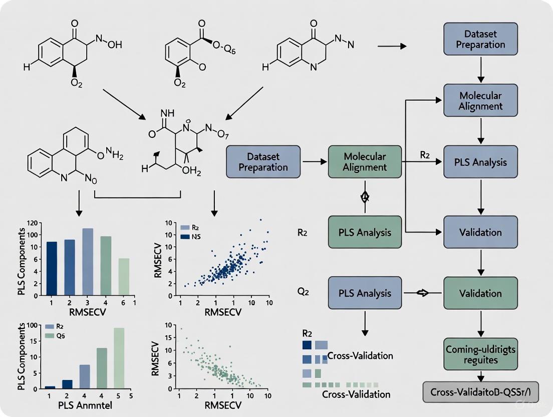
The following diagram illustrates the comprehensive workflow for developing 3D-QSAR models using PLS regression, integrating both model building and validation phases:
PLS Component Optimization Procedure
Optimizing the number of PLS components represents a critical step in model development to balance model complexity with predictive power. The following protocol outlines a standardized approach:
Step 1: Data Preprocessing Standardize both predictor and response variables to mean-centered distributions with unit variance. This ensures that variables measured on different scales contribute equally to the model [6].
Step 2: Initial Model Fitting
Fit a PLS model with the maximum number of components (up to the number of predictors). In R, this can be implemented using the plsr() function from the pls package:
Step 3: Cross-Validation Perform k-fold cross-validation (typically 5-10 folds) to evaluate model performance with different numbers of components. Record the Root Mean Squared Error of Prediction (RMSEP) for each component count [6].
Step 4: Optimal Component Selection Identify the number of components that minimizes the cross-validated RMSEP. As shown in Table 2, the optimal balance typically occurs when adding more components does not significantly improve predictive performance.
Step 5: Model Validation Validate the final model with the selected number of components using an external test set not used during model development. Calculate performance metrics including R² (goodness of fit) and Q² (predictive ability) [1] [5].
Table 2: Example Cross-Validation Results for PLS Component Selection
| Number of Components | Test RMSEP | R² (Training) | Q² (Cross-Validation) | Variance Explained in X | Variance Explained in Y |
|---|---|---|---|---|---|
| 1 | 40.57 | 0.6866 | 0.7184 | 68.66% | 71.84% |
| 2 | 35.48 | 0.8927 | 0.8174 | 89.27% | 81.74% |
| 3 | 36.22 | 0.9582 | 0.8200 | 95.82% | 82.00% |
| 4 | 36.74 | 0.9794 | 0.8202 | 97.94% | 82.02% |
| 5 | 36.67 | 1.0000 | 0.8203 | 100.00% | 82.03% |
Troubleshooting Guides and FAQs
Common Experimental Challenges and Solutions
Q1: My PLS model shows excellent fit but poor predictive performance. What might be causing this overfitting and how can I address it?
A: Overfitting typically occurs when the model contains too many components relative to the number of observations or when descriptors with minimal predictive value are included. Implement the following solutions:
- Apply rigorous descriptor selection: Use genetic algorithms for descriptor selection to eliminate irrelevant variables that contribute to noise rather than signal [1]. The genetic algorithm approach implemented in MFTA software can reduce descriptor count by 5-10 fold while maintaining or improving predictivity.
- Optimize component count: Determine the optimal number of PLS components through cross-validation rather than using the maximum possible. The optimal number typically corresponds to the minimum in cross-validated error (Figure 1).
- Increase validation rigor: Replace leave-one-out cross-validation with more robust k-fold cross-validation (k=5-10) or repeated double cross-validation, as LOOCV may overestimate predictivity [1] [7].
Q2: How should I handle highly correlated 3D descriptors in my PLS model?
A: Unlike traditional regression, PLS regression is specifically designed to handle correlated predictors. However, extreme correlation can still cause instability. Consider these approaches:
- Retain correlated descriptors: PLS components are linear combinations of original descriptors, and the method is robust to correlations between them [1] [3].
- Apply variance-based filtering: Remove descriptors with near-zero variance that provide no meaningful information [1].
- Standardize descriptors: Ensure all descriptors are standardized (mean-centered and scaled to unit variance) before model building to prevent dominance by high-variance variables [6].
Q3: What is the difference between Q² and R² in PLS model validation, and which should I prioritize?
A: These metrics serve distinct purposes in model evaluation:
- R² (coefficient of determination): Measures how well the model explains variance in the training data. High R² indicates good fit but does not guarantee predictive power.
- Q² (cross-validated R²): Assesses predictive performance on data not used in model building. Calculated as 1 - (PRESS/SSY), where PRESS is the prediction error sum of squares and SSY is the total sum of squares of Y [1].
Prioritize Q² as the primary metric for model selection, as it better indicates real-world predictive performance. A robust QSAR model should have Q² > 0.5, with values above 0.7 considered excellent [7] [5].
Q4: How can I interpret the contribution of individual molecular descriptors in a PLS model when the model uses latent variables?
A: Although PLS models use latent variables, you can trace back the contribution of original descriptors through several methods:
- Variable Importance in Projection (VIP): Calculate VIP scores that quantify each descriptor's contribution across all components. Descriptors with VIP > 1.0 are generally considered significant [3].
- Regression coefficients: Transform the PLS model back to original descriptor space to obtain standardized regression coefficients that indicate the direction and magnitude of each descriptor's effect [1].
- Contour maps: For 3D-QSAR models, visualize coefficient values spatially to identify regions where specific molecular features (steric bulk, electronegativity) enhance or diminish activity [5].
Q5: What are the common pitfalls in molecular alignment for 3D-QSAR, and how do they affect PLS models?
A: Molecular alignment represents one of the most critical and challenging steps in 3D-QSAR. Common issues include:
- Incorrect bioactive conformation: Using low-energy conformations rather than putative bioactive conformations can misalign key functional groups. Solution: Employ docking studies or pharmacophore modeling to guide conformation selection [5].
- Inconsistent alignment: Slight variations in alignment can dramatically alter descriptor values. Solution: Use robust alignment methods like maximum common substructure (MCS) or field-based alignment [5].
- Diverse binding modes: Assuming identical binding modes for structurally diverse compounds. Solution: For highly diverse datasets, consider alignment-independent descriptors or cluster compounds by suspected binding mode.
Alignment errors manifest in PLS models as poor predictive performance and inconsistent structure-activity relationships, as the mathematical model cannot compensate for fundamental spatial misrepresentation of molecular features.
Advanced Troubleshooting: Optimization of PLS Components
The following diagram illustrates the decision process for optimizing PLS components during model building, addressing the core thesis of component optimization in validation research:
Q6: How do I determine if I need more PLS components in my model?
A: Evaluate these diagnostic indicators:
- Cross-validation metrics: Add components until the cross-validated Q² reaches a plateau or begins to decrease. The optimal number typically occurs at the "elbow" point where additional components provide diminishing returns [1] [6].
- RMSEP plot: Plot Root Mean Squared Error of Prediction against component count. The minimum point indicates the optimal number (see Table 2 for example).
- Variance explanation: Monitor the percentage of Y-variance explained. While X-variance continues to increase with additional components, the relevant Y-variance typically plateaus.
Q7: What is the relationship between the number of descriptors, number of compounds, and optimal PLS components?
A: The optimal number of PLS components should be significantly less than both the number of compounds and the number of descriptors. As a general guideline:
- Minimum observations: 5-10 compounds per PLS component to ensure model stability [1]
- Component limit: The maximum number of meaningful PLS components cannot exceed the number of compounds in the training set
- Descriptor reduction: For datasets with thousands of descriptors (common in 3D-QSAR), apply feature selection before PLS to reduce the descriptor set to 50-100 most relevant variables [7]
Table 3: Essential Software Tools for 3D-QSAR with PLS Regression
| Tool Name | Type | Primary Function | Application in PLS-based QSAR |
|---|---|---|---|
| Sybyl-X | Commercial Software | Molecular modeling and 3D-QSAR | CoMFA and CoMSIA analysis, molecular alignment, PLS regression [8] [5] |
| RDKit | Open-source Cheminformatics | Molecular descriptor calculation | 2D/3D descriptor generation, maximum common substructure alignment [5] |
| alvaDesc | Commercial Descriptor Package | Molecular descriptor calculation | Calculation of >4000 molecular descriptors for QSAR modeling [4] |
| Dragon | Commercial Software | Molecular descriptor calculation | Calculation of 5,270 molecular descriptors for LINUX and WIN platforms [4] |
| PaDEL-Descriptor | Open-source Software | Molecular descriptor calculation | Calculation of 2D and 3D descriptors based on CDK library [4] |
| R pls package | Open-source Statistical Package | PLS regression analysis | Model building, cross-validation, component optimization [6] |
| Open3DQSAR | Open-source Tool | Pharmacophore modeling | Molecular interaction field calculation for 3D-QSAR [4] |
Table 4: Critical Statistical Metrics for PLS Model Validation
| Metric | Formula | Interpretation | Optimal Range |
|---|---|---|---|
| R² (Coefficient of Determination) | R² = 1 - (SSres/SStot) | Goodness of fit for training data | > 0.7 for reliable models |
| Q² (Cross-validated R²) | Q² = 1 - (PRESS/SStot) | Predictive ability on unseen data | > 0.5 (acceptable), > 0.7 (excellent) |
| RMSEP (Root Mean Square Error of Prediction) | RMSEP = √(∑(yᵢ-ŷᵢ)²/n) | Average prediction error | Lower values indicate better performance |
| VIP (Variable Importance in Projection) | VIP = √(p∑(SSbₕwₕ²)/∑SSbₕ²) | Contribution of each original variable | Variables with VIP > 1.0 are significant |
| SEE (Standard Error of Estimate) | SEE = √(SSres/(n-p-1)) | Precision of regression coefficients | Lower values indicate better precision |
Frequently Asked Questions (FAQs)
1. What is the primary advantage of using PLS over Multiple Linear Regression (MLR) in QSAR? PLS is specifically designed to handle data where the number of molecular descriptors exceeds the number of compounds and when these descriptors are highly correlated (multicollinear) [9] [10]. Unlike MLR, which becomes unstable or fails under these conditions, PLS creates a set of orthogonal latent variables (components) that maximize the covariance between the predictor variables (X) and the response variable (Y) [11] [12]. This makes it particularly suitable for QSAR models built from a large number of correlated 2D or 3D molecular descriptors [9] [13].
2. My 3D-QSAR model is overfitting. How can PLS help? Overfitting often occurs when a model has too many parameters relative to the number of observations. PLS combats this through dimensionality reduction. It extracts a small number of latent components that capture the essential variance in the descriptor data that is relevant for predicting biological activity [9]. The key is to optimize the number of PLS components, typically using cross-validation techniques to find the point that maximizes predictive performance without modeling noise [9] [14].
3. How do I determine the optimal number of PLS components for my model? The optimal number of components is found through cross-validation [9] [14]. A common method is k-fold cross-validation:
- Split your training set into k subsets (e.g., 5 folds).
- Train the PLS model on k-1 folds using a provisional number of components.
- Predict the held-out fold and calculate the error.
- Repeat this process until each fold has been left out once.
- Calculate the overall cross-validated correlation coefficient (Q²) and standard error.
- Repeat for different numbers of components.
- The number of components that gives the highest Q² value (or lowest error) is considered optimal [9]. This process is automated in many software packages like
rQSAR[14].
4. What are the key statistical metrics for validating a PLS-based QSAR model? A robust PLS-QSAR model should be evaluated using both internal and external validation metrics, summarized in the table below.
Table 1: Key Validation Metrics for PLS-QSAR Models
| Metric | Description | Interpretation |
|---|---|---|
| R² | Coefficient of determination for the training set | Goodness-of-fit for the training data [8] [13]. |
| Q² | Cross-validated correlation coefficient | Estimate of the model's predictive power and robustness [8] [13]. |
| SEE | Standard Error of Estimate | Measures the accuracy of the model for the training set [8]. |
| F Value | Fisher F-test statistic | Significance of the overall model [8]. |
| R²Test | Coefficient of determination for an external test set | The most reliable measure of a model's predictive ability on new data [9] [15]. |
5. Can PLS capture non-linear structure-activity relationships? Standard PLS is a linear method. However, several non-linear extensions have been developed to overcome this limitation, as shown in the table below [10].
Table 2: Common Non-Linear Extensions of PLS
| Method | Key Feature | Application in QSAR |
|---|---|---|
| Kernel PLS (KPLS) | Maps data to a high-dimensional feature space using kernel functions [10]. | Suitable for complex, non-linear relationships [10]. |
| Neural Network-based NPLS | Uses neural networks to extract non-linear latent variables or for regression [10]. | Captures intricate, hierarchical patterns in data [10]. |
| PLS with Spline Transformation | Uses spline functions for piecewise linear regression [10]. | Provides flexibility and good interpretability [10]. |
Troubleshooting Guides
Problem: Low Predictive Performance on External Test Set A model with good internal cross-validation statistics (Q²) may still perform poorly on new, unseen compounds. This is a sign of limited generalizability.
- Potential Cause 1: The model is built on molecular descriptors that are not sufficiently relevant to the biological activity, or it lacks key descriptors.
Solution: Perform rigorous feature selection before PLS modeling. Use methods like Genetic Algorithms (GA) [12] or filter methods based on correlation to identify and retain the most informative descriptors. This improves model interpretability and can enhance predictive performance [9].
Potential Cause 2: The model's Applicability Domain (AD) is not well-defined, and predictions are being made for compounds structurally different from the training set.
- Solution: Define the applicability domain of your model. This can be based on the leverage of compounds or their distance in the descriptor space. Clearly state that predictions for compounds outside this domain are unreliable [9].
Problem: Unstable Model - Small Changes in Data Lead to Large Changes in Results Model instability undermines its reliability for virtual screening or chemical design.
- Potential Cause: High leverage from outliers or an insufficient number of training compounds relative to the complexity of the structure-activity relationship.
- Solution:
- Check for Outliers: Analyze the model's residuals and leverage (Hat values) to identify influential compounds that may be distorting the model. Investigate these compounds for potential errors in structure or activity data [9].
- Increase Training Set Size and Diversity: If possible, curate a larger and more chemically diverse training set that adequately represents the chemical space of interest [9].
- Use Robust PLS Variants: Consider methods like Genetic Partial Least Squares (G/PLS), which combines genetic algorithm-based variable selection with PLS regression to build more stable and predictive models [12].
Problem: Difficulty Interpreting the PLS Model in a Chemically Meaningful Way While PLS is a "grey box" model, it should still offer insights into the Structural Features influencing activity.
- Potential Cause: Relying solely on the model's regression coefficients, which can be difficult to interpret when descriptors are correlated.
- Solution:
- Analyze Variable Importance in Projection (VIP): The VIP score measures the contribution of each descriptor to the PLS model. Focus on descriptors with a VIP score > 1.0, as these are the most relevant for explaining the activity [13].
- Visualize Contour Maps (for 3D-QSAR): If using 3D-QSAR methods like CoMFA or CoMSIA, the PLS coefficients can be visualized as 3D contour maps around a molecular scaffold. These maps intuitively show regions where specific chemical features (e.g., steric bulk, electropositive groups) increase or decrease biological activity [8].
Experimental Protocol: Developing and Validating a PLS-based 3D-QSAR Model
The following workflow, based on a recent study on MAO-B inhibitors [8], details the key steps for building a robust PLS model within a 3D-QSAR framework.
Figure 1: PLS-based 3D-QSAR Model Development Workflow
Step-by-Step Methodology:
Dataset Curation and Preparation
- Curate a set of molecules with known biological activities (e.g., IC₅₀, pIC₅₀) [9] [8].
- Standardize chemical structures: remove salts, normalize tautomers, define protonation states [9].
- For 3D-QSAR, generate low-energy 3D conformers for each compound. A common approach is to use the global minimum of the potential energy surface [15].
Molecular Alignment and Descriptor Calculation
- Align all molecules to a common template or a active reference molecule in the database. This is a critical step for 3D-QSAR methods like CoMFA and CoMSIA [8].
- Calculate 3D molecular field descriptors (e.g., steric, electrostatic, hydrophobic) using software such as Sybyl-X [8]. This generates a high-dimensional matrix (X) of molecular descriptors.
Data Set Partitioning
- Divide the dataset into a training set (typically ~80%) for model building and a test set (~20%) for external validation. Use methods like the Kennard-Stone algorithm to ensure the test set is representative of the chemical space covered by the training set [9].
PLS Model Construction and Cross-Validation
- Use the training set to build the initial PLS model, which finds latent variables that maximize covariance between the molecular fields (X) and biological activity (Y) [11] [8].
- Perform leave-one-out (LOO) or k-fold cross-validation to determine the optimal number of PLS components. The model with the highest cross-validated correlation coefficient (q² or Q²) is selected [8]. The statistical results from a published MAO-B inhibitor study are shown below.
Table 3: Exemplary PLS Model Statistics from a 3D-QSAR Study [8]
| Model | q² | r² | SEE | F Value | Optimal PLS Components |
|---|---|---|---|---|---|
| COMSIA | 0.569 | 0.915 | 0.109 | 52.714 | Reported as part of the model |
External Model Validation
Model Interpretation and Deployment
The Scientist's Toolkit: Essential Research Reagents & Software
Table 4: Key Software Tools for PLS-QSAR Modeling
| Tool Name | Type/Function | Use Case in PLS-QSAR |
|---|---|---|
| Sybyl-X | Molecular Modeling Suite | Performing 3D-QSAR (CoMFA, CoMSIA) and generating 3D molecular field descriptors for PLS regression [8]. |
| rQSAR (R Package) | Cheminformatics & Modeling | Building QSAR models using PLS, MLR, and Random Forest directly from molecular structures and descriptor tables [14]. |
| PaDEL-Descriptor | Descriptor Calculation Software | Generating a wide range of 1D and 2D molecular descriptors from chemical structures for input into PLS models [9]. |
| DRAGON | Molecular Descriptor Software | Calculating thousands of molecular descriptors for QSAR modeling; often used with PLS for variable reduction [13]. |
| COMSIA Method | 3D-QSAR Methodology | A specific 3D-QSAR technique that relies on PLS regression to correlate molecular similarity fields with biological activity [8]. |
Frequently Asked Questions
FAQ 1: Why does the total variance explained by all my PLS components not add up to 100%?
This is an expected behavior of Partial Least Squares (PLS) regression, not an error in your model. Unlike Principal Component Analysis (PCA), which creates components with orthogonal weight vectors to maximize explained variance in the predictor variable (X), PLS creates components with non-orthogonal weight vectors to maximize covariance between X and the response variable (Y) [16]. Because these weight vectors are not orthogonal, the variance explained by each PLS component overlaps, and the sum of variances for all components will be less than the total variance in the original dataset [16]. A robust PLS model for prediction does not require the components to explain 100% of the variance in X.
FAQ 2: How many PLS components should I select for a robust 3D-QSAR model?
Selecting the optimal number of components is critical to avoid overfitting. The goal is to find the point where adding more components no longer significantly improves the model's predictive power [3].
A standard methodology is to use k-fold cross-validation [5] [9]. The detailed protocol is:
- Define a range of component numbers to test (e.g., 1 to 10).
- For each number of components (
n) in this range, perform k-fold cross-validation on the training set. - Build a PLS model with
ncomponents on k-1 folds and predict the held-out fold. - Calculate the mean squared error (MSE) or the cross-validated correlation coefficient (Q²) for each
n. - Plot the performance metric (e.g., MSE) against the number of components.
- Select the number of components where the MSE is minimized or where the Q² value is maximized. Adding more components beyond this point typically leads to overfitting [3].
FAQ 3: What is the practical difference between a latent variable in PLS and a principal component in PCA?
Both are latent variables, but they are constructed with different objectives, which has direct implications for 3D-QSAR.
The table below summarizes the key differences:
| Feature | PLS (Partial Least Squares) | PCA (Principal Component Analysis) |
|---|---|---|
| Primary Goal | Maximize covariance with the response (Y) [3]. | Maximize variance in the descriptor data (X). |
| Model Role | Used for supervised regression; components are directly relevant to predicting activity [17]. | Used for unsupervised dimensionality reduction; components may not be relevant to activity. |
| Output | A predictive model linking X to Y. | A transformed, lower-dimensional representation of X. |
In 3D-QSAR, PLS is preferred because it directly uses the biological activity data (Y) to shape the latent variables, ensuring they are relevant for prediction [5] [18].
FAQ 4: My 3D-QSAR model has a high R² but poor predictive ability. What might be wrong?
This is a classic sign of overfitting. Your model has memorized the noise in the training data instead of learning the generalizable structure-activity relationship.
Troubleshooting steps include:
- Reduce Model Dimensionality: You may be using too many PLS components. Re-run the cross-validation to ensure the optimal number of components is selected [3].
- Check Applicability Domain: The new compounds you are predicting may fall outside the chemical space of the compounds used to train the model. The model's predictions for these compounds are unreliable [9].
- Validate the Alignment: For 3D-QSAR methods like CoMFA, a poor molecular alignment is a primary source of error and can lead to non-predictive models [5].
Experimental Protocol: Building and Validating a 3D-QSAR Model
This protocol outlines the key steps for developing a 3D-QSAR model using PLS regression.
1. Data Collection and Preparation
- Assemble a Dataset: Collect a series of compounds with experimentally determined biological activities (e.g., IC₅₀, Ki) measured under uniform conditions [5].
- Calculate 3D Descriptors:
- Generate a low-energy 3D conformation for each molecule [5].
- Align all molecules to a common reference frame based on a putative bioactive conformation [5].
- Calculate 3D molecular field descriptors using a method like CoMFA (steric and electrostatic fields) or CoMSIA (additional fields like hydrophobic, H-bond donor/acceptor) [5] [8].
2. Model Building and Optimization
- Split Data: Divide the dataset into a training set (for model building) and an independent test set (for final validation) [9].
- Perform Feature Selection (Optional): Use Variable Importance in Projection (VIP) scores from a preliminary PLS model to identify and retain only the most relevant descriptors [3].
- Determine Optimal PLS Components:
- Use the k-fold cross-validation method described in FAQ 2 on your training set.
- The optimal number of components is identified by the model with the highest cross-validated Q² value [5].
3. Model Validation and Interpretation
- Build Final Model: Construct the final PLS model using the optimal number of components on the entire training set.
- External Validation: Use the held-out test set to evaluate the model's predictive power. Report R² and RMSE for the test set predictions [19] [8].
- Interpret Contour Maps: Visualize the 3D-QSAR model as contour maps. These maps show regions where specific molecular properties (steric bulk, positive charge, etc.) are favorable or unfavorable for biological activity, providing a guide for chemical modification [5].
3D-QSAR Model Development Workflow
The Scientist's Toolkit: Essential Research Reagents & Software
The following table lists key software tools and their functions for 3D-QSAR modeling.
| Tool Name | Function in 3D-QSAR | Reference |
|---|---|---|
| Sybyl-X | A comprehensive molecular modeling suite used for structure building, geometry optimization, molecular alignment, and performing CoMFA/CoMSIA studies [5] [8]. | [5] [8] |
| RDKit | An open-source cheminformatics toolkit. Used for generating 2D and 3D molecular structures, calculating 2D descriptors, and performing maximum common substructure (MCS) searches for alignment [5] [20]. | [5] [20] |
| MATLAB (plsregress) | A high-level programming platform. Its plsregress function is used to perform PLS regression and calculate the percentage of variance explained (PCTVAR) by each component [21]. |
[21] |
| scikit-learn / OpenTSNE | Python libraries for machine learning. scikit-learn provides PCA and other utilities, while OpenTSNE offers efficient implementations of t-SNE for chemical space visualization [20]. | [20] |
The 3D-QSAR Design-Iterate Loop
The Critical Link Between PLS Components and Model Predictivity
Frequently Asked Questions (FAQs)
1. What is the fundamental role of PLS components in a 3D-QSAR model? PLS components are latent variables that serve as the foundational building blocks of a 3D-QSAR model. They are linear combinations of the original 3D molecular field descriptors (steric, electrostatic, hydrophobic, etc.) that are constructed with a specific goal: to maximize the covariance between the predictor variables (X) and the biological activity response (y). Unlike methods like Principal Component Regression (PCR) that only consider the variance in X, PLS explicitly uses the response variable y to guide the creation of components, ensuring they are relevant predictors of biological activity [22] [23].
2. How does the number of PLS components directly impact model predictivity? Selecting the optimal number of PLS components is critical to balancing model fit and predictive ability.
- Too few components lead to underfitting, where the model is too simple to capture the essential structure-activity relationship, resulting in high prediction errors for both training and new compounds [22].
- Too many components lead to overfitting, where the model starts to fit the noise in the training data rather than the underlying trend. While it may perfectly predict the training set, its performance will drop significantly when applied to new, unseen test data [22]. A robust model achieves a low estimated prediction error on an external test set, which is typically found at an intermediate, optimal number of components [23].
3. What are the key statistical metrics for validating a PLS-based 3D-QSAR model? A valid 3D-QSAR model should be evaluated using a suite of metrics, not just a single one [24]. The most common are:
- q² (Q²): The cross-validated coefficient of determination (e.g., from Leave-One-Out validation). It estimates the model's predictive power from the training process. A value above 0.5 is generally considered acceptable [8] [25].
- r² (R²): The conventional coefficient of determination for the training set. It measures the goodness-of-fit [8] [25].
- r²pred: The coefficient of determination for an external test set. This is the most reliable measure of a model's real predictive power for new compounds [25].
- SEE (or S): The Standard Error of Estimate, which indicates the average accuracy of the predictions [8].
The following table summarizes benchmark values from a robust 3D-QSAR study on steroids using the CoMSIA method:
Table 1: Benchmark Validation Metrics from a CoMSIA Study on Steroids [25]
| Metric | Reported Value | Interpretation |
|---|---|---|
| q² | 0.609 | Good internal predictive ability |
| r² | 0.917 | Excellent fit to the training data |
| SEE (S) | 0.33 | Low estimation error |
| Optimal Number of Components | 3 | Model of optimal complexity |
4. My model has a high R² but poor predictive power for new compounds. What is the most likely cause? This is a classic sign of overfitting [22]. Your model has likely been trained with too many PLS components, causing it to memorize the training data, including its experimental noise, instead of learning the generalizable structure-activity relationship. To fix this, you must re-evaluate your model using cross-validation or an external test set to find the optimal, lower number of components that minimizes the prediction error for new data [24] [22].
Troubleshooting Guides
Issue 1: How to Determine the Optimal Number of PLS Components
Detailed Protocol: The most statistically sound method for choosing the number of components is cross-validation (CV). The following workflow, which can be implemented in tools like R or Python, is recommended [22] [23]:
Figure 1: The workflow illustrates the process of determining the optimal number of PLS components through cross-validation, starting from data preparation, iterating through different component numbers, performing cross-validation to calculate MSEP, and finally selecting the number with the lowest MSEP for model building and validation.
- Prepare Data: Split your dataset into a training set and a separate, external test set. The test set will be used for final validation only.
- Iterate Component Numbers: For a reasonable range of component numbers (e.g., 1 to 10 or 15), perform k-fold cross-validation (e.g., 10-fold) on the training set.
- Calculate MSEP: For each number of components, calculate the Mean Squared Prediction Error (MSEP) across all cross-validation folds.
- Plot and Identify Minimum: Plot the MSEP values against the number of components. The optimal number is the one that minimizes the MSEP. Sometimes, a parsimonious choice is the number of components where the MSEP curve first plateaus or is not significantly worse than the minimum.
- Build and Validate: Build your final model on the entire training set using the optimal number of components. Finally, assess its predictivity using the held-out external test set by calculating r²pred [23].
Issue 2: Low q² and r²pred Values After Model Construction
A model with low predictive power (q² and r²pred < 0.5) indicates fundamental issues. Follow this diagnostic flowchart to identify and resolve the problem.
Figure 2: This decision tree helps diagnose the root cause of a model with low predictive power (low q² and r²pred), guiding the user to check for issues in data quality, molecular alignment, descriptor selection, and the final model validation step.
Potential Causes and Solutions:
- Data Quality Problem: The biological activity data may come from inconsistent experimental assays or have a narrow range, making it difficult to find a meaningful correlation [5]. Solution: Re-check and curate your input data, ensuring all activities were measured under uniform conditions and cover a wide enough potency range.
- Poor Molecular Alignment: In 3D-QSAR, the alignment of molecules is a critical and sensitive step. An incorrect alignment, which does not reflect the true bioactive conformations, will produce meaningless field descriptors [5]. Solution: Re-visit your alignment strategy. Use a robust maximum common substructure (MCS) algorithm or docked conformations to achieve a pharmacologically relevant alignment [5].
- Insufficient Molecular Descriptors: The chosen molecular fields (e.g., only steric and electrostatic) might not capture the key interactions governing binding affinity. Solution: Consider using the extended fields available in methods like CoMSIA, which include hydrophobic, and hydrogen-bond donor and acceptor fields, to provide a more holistic view of the interactions [25] [26].
The Scientist's Toolkit: Essential Research Reagents & Software
Table 2: Key computational tools and methods for developing and validating 3D-QSAR models.
| Tool/Method | Type | Primary Function in 3D-QSAR |
|---|---|---|
| Sybyl (Tripos) | Proprietary Software Suite | The historical industry standard for performing CoMFA and CoMSIA analyses, providing integrated tools for alignment, field calculation, and PLS regression [25]. |
| Py-CoMSIA | Open-Source Python Library | A modern, open-source implementation of CoMSIA that increases accessibility and allows for customization of the 3D-QSAR workflow [25]. |
| RDKit | Open-Source Cheminformatics Library | Used for generating 3D molecular structures from 2D representations, energy minimization (using UFF), and identifying maximum common substructures (MCS) for alignment [5]. |
| PLS Regression | Statistical Algorithm | The core multivariate regression method used to correlate 3D field descriptors with biological activity and build the predictive model [5] [22]. |
| Cross-Validation (e.g., LOOCV, 10-fold) | Validation Technique | A crucial method for estimating the predictive performance of a model during training and for selecting the optimal number of PLS components without overfitting [22] [23]. |
| Comparative Molecular Similarity Indices Analysis (CoMSIA) | 3D-QSAR Method | An advanced 3D-QSAR technique that uses Gaussian functions to calculate steric, electrostatic, hydrophobic, and hydrogen-bonding fields, often providing more interpretable and robust models than its predecessor, CoMFA [25] [26]. |
A Step-by-Step Guide to Building and Optimizing Your PLS 3D-QSAR Model
Frequently Asked Questions
Q1: What are the minimum data point requirements for calculating valid 3D descriptors and building reliable 3D-QSAR models? A sufficient number of data points is critical for a robust model. The absolute minimums are guided by the complexity of the molecular shape you are trying to fit [27].
- Cylinder: 5 points
- Cone: 6 points
- Sphere: 4 points
- Plane: 3 points
Using only the absolute minimum points will result in a measured shape error of zero, which is not realistic. It is recommended to densely measure features with more points to capture true shape variations for effective fitting in your 3D-QSAR studies [27].
Q2: My dataset contains both continuous (e.g., IC50) and categorical (e.g., active/inactive) biological activity data. How should I structure this for analysis? You must first determine the nature of your data, as this dictates the visualization and analysis approach [28]. Biological activity data typically falls into these categories:
- Quantitative Data (IC50, pIC50): These are ratio-level data. They have an absolute zero (no activity) and you can meaningfully calculate ratios (e.g., a 10 nM IC50 is ten times more potent than a 100 nM IC50).
- Qualitative/Categorical Data (Active/Inactive): These are nominal or ordinal data. For example, classifying compounds as "Active," "Inactive," or "Intermediate" represents an ordinal scale.
For 3D-QSAR, pIC50 (-logIC50) is the preferred continuous variable because it linearizes the relationship with binding energy [29].
Q3: What is the recommended color palette for visualizing different data types in my 3D-QSAR results? Using color palettes aligned with your data type prevents misinterpretation [28].
- Table 1: Recommended Color Palettes for Biological Data Visualization
| Data Type | Example | Recommended Palette | Purpose |
|---|---|---|---|
| Sequential | pIC50 values (low to high) | Viridis | Shows ordered data from lower to higher values. Luminance increases monotonically. |
| Diverging | Residuals (negative vs. positive) | ColorBrewer Diverging | Highlights deviation from a median value (e.g., mean activity). |
| Qualitative | Different protein targets | Tableau 10 | Distinguishes between categories with no inherent order. |
These palettes are perceptively uniform and friendly to users with color vision deficiencies [28].
Q4: How do I handle errors related to "feature direction" or "polar axis" during 3D descriptor alignment? This error arises when the alignment of your molecules does not match the polar coordinate system defined by your 3D-QSAR software [27]. To resolve this:
- Ensure all molecules are aligned such that their dominant axes are nominally parallel to the polar axis defined by the common framework.
- The benchmark reference frame must define a clear polar origin. Check that your alignment protocol correctly establishes this axis.
- If your molecules are coaxial with the alignment axis, a radial (diameter-based) tolerance zone might be more appropriate than a polar one [27].
Troubleshooting Guides
Problem: Low Correlation or Poor Model Performance During 3D-QSAR Validation Poor performance can stem from issues in data curation, descriptor calculation, or model optimization.
Potential Cause 1: Incorrect or Inconsistent Biological Activity Data.
- Solution: Implement a rigorous data curation protocol.
- Protocol: Standardize activity measures (e.g., consistently use pIC50 over IC50). Identify and handle outliers using statistical methods (e.g., Z-scores). Verify that all data points are from comparable experimental assays (e.g., same cell line, pH, incubation time).
Potential Cause 2: Inadequate Constraint of Molecular Conformation and Alignment.
- Solution: Ensure your molecular alignment protocol properly constrains all degrees of freedom.
- Protocol: The benchmark reference frame used for aligning molecules must fully define the orientation. If the software reports that the "benchmark reference frame must define a clear polar origin," review your alignment rules. As noted in troubleshooting guides, "Ensure the benchmark reference frame defines a clear polar axis" [27].
Potential Cause 3: Suboptimal Number of PLS Components.
- Solution: Systematically determine the optimal number of PLS components to avoid overfitting or underfitting.
- Protocol: Use cross-validation (e.g., leave-one-out or group cross-validation). The optimal number of components is typically indicated by the number that gives the minimum cross-validated standard error of prediction. A scree plot of the cross-validated correlation coefficient (q²) against the number of components can visually identify the point where adding more components no longer significantly improves the model.
Problem: "Feature点数过少, 无法有效拟合" (Insufficient Feature Points for Effective Fitting) This error indicates that a molecular feature or descriptor does not have enough data points to define its 3D shape uniquely [27].
- Potential Cause: The molecular structure or the field around it has been sampled with too few points for the software to perform a reliable fit.
- Solution:
- Increase the density of points used to represent the molecular structure or its interaction fields.
- For complex, nearly symmetric surfaces, ensure the benchmark reference frame uses other benchmarks to constrain the uncertain degrees of freedom [27].
- Refer to the minimum point requirements in FAQ #1 as a baseline and exceed them where possible.
Problem: "特征方向必须与其对应的极坐标公差带匹配" (Feature Direction Must Match Polar Tolerance Zone) This error is related to the incorrect orientation of molecules or their descriptors relative to the defined alignment axis [27].
- Potential Cause: The theoretical (THEO) direction of the molecular feature or the entire molecule is not parallel to the polar axis established by the benchmark reference frame.
- Solution:
- Check the nominal orientation of your aligned molecules in the software.
- Ensure the alignment protocol correctly constrains the primary molecular axis to the polar axis of the system. The software expects that "all molecular features must nominally be parallel to the polar axis defined by the benchmark reference frame" [27].
- If the issue persists, review the fundamental alignment rules in your molecular spreadsheet.
The Scientist's Toolkit
- Table 2: Essential Research Reagent Solutions for 3D-QSAR
| Item | Function in 3D-QSAR Workflow |
|---|---|
| Curated Bioactivity Database (e.g., ChEMBL) | Provides publicly available, standardized bioactivity data (e.g., IC50, Ki) for model building and validation. |
| Molecular Spreadsheet Software (e.g., Sybyl) | The core environment for storing molecular structures, calculated descriptors, and biological activity data, and for performing statistical analysis. |
| 3D-QSAR Software with CoMFA/CoMSIA | Enables the calculation of steric, electrostatic, and other molecular interaction fields (MIFs) that form the 3D descriptors for the model [29]. |
| Docking Software (e.g., AutoDock Vina) | Used to generate a common alignment hypothesis for molecules by docking them into a protein's active site, which can then be used for 3D descriptor calculation. |
| Geometry Optimization Software (e.g., Gaussian) | Used to calculate the minimal energy 3D conformation of each molecule, which is a critical first step before alignment and descriptor calculation [29]. |
Workflow and Troubleshooting Diagrams
The following diagram illustrates the core workflow for data preparation and the key troubleshooting checkpoints.
3D-QSAR Data Prep and Troubleshooting
When a troubleshooting step is triggered (e.g., a "Descriptor Error"), the following detailed logic path should be followed to resolve the issue.
Resolving 3D Descriptor Calculation Errors
Frequently Asked Questions (FAQs)
Q1: Why is molecular alignment considered the most critical step in CoMFA/CoMSIA studies? Molecular alignment is the foundation of CoMFA/CoMSIA because these methods are highly alignment-dependent [30]. The three-dimensional fields (steric, electrostatic, etc.) that are calculated and correlated with biological activity are entirely determined by the spatial orientation of the molecules. An incorrect alignment introduces significant noise into the descriptor matrix, leading to models with little to no predictive power. The signal in a 3D-QSAR model primarily comes from the alignments themselves [31].
Q2: What are the common methods available for aligning molecules? Several methods are commonly used for molecular alignment, each with its own strengths:
- Atom-Based Superimposition: This method involves atom-to-atom pairing between molecules, typically aligning a common structural core or pharmacophore [32].
- Field and Shape-Guided Alignment: This approach uses molecular fields (steric and electrostatic) and overall molecular shape to find the optimal superposition, often resulting in a more biologically relevant alignment than rigid atom-based methods [31].
- Field Fit Procedure: This technique minimizes the differences in the calculated steric and electrostatic fields between various molecules to achieve an optimal alignment [33].
Q3: I have an outlier in my model with poor predictive activity. Should I realign it to improve the fit? No. This is a common but critical error. You must not alter the alignment of any molecule based on the output of the model (i.e., its predicted activity) [31]. Doing so biases the model by making the input data (the alignments) dependent on the output data (the activities), which invalidates the model's statistical validity and predictive power. Alignment must be fixed before running the QSAR analysis, and activities should be ignored during the alignment process.
Q4: What is the key difference in the fields calculated by CoMFA and CoMSIA? The key difference lies in the potential functions used:
- CoMFA uses Lennard-Jones (steric) and Coulombic (electrostatic) potentials. These potentials can be very steep near the molecular surface, leading to singularities and requiring the user to define arbitrary cutoff limits [30] [32].
- CoMSIA uses a Gaussian-type distance dependence for all its fields (steric, electrostatic, hydrophobic, H-bond donor, H-bond acceptor). This results in much "softer" potentials without singularities, which avoids the issues of cutoffs and steep gradients [30] [34].
Q5: How do the interpretation of CoMFA and CoMSIA contour maps differ? The contour maps provide different guides for design:
- CoMFA maps indicate regions in space around the aligned molecules where interactions with a putative receptor environment are favored or disfavored [30].
- CoMSIA maps highlight regions within the area occupied by the ligand skeletons that require a specific physicochemical property for high activity. This is often a more direct guide for modifying the ligand structure itself [30] [34].
Troubleshooting Guide
Poor Model Predictivity (q²orr²pred)
| Symptom | Possible Cause | Solution |
|---|---|---|
Low cross-validated correlation coefficient (q²) and poor predictive r² for the test set. |
Incorrect or inconsistent molecular alignment. This is the most common source of failure. | Re-check all alignments visually and based on chemical intuition. Use multiple reference molecules to constrain the alignment of the entire set [31]. |
| The chosen bioactive conformation is incorrect for one or more molecules. | Re-visit conformational analysis. If available, use experimental data (e.g., X-ray crystallography, NMR) or docking poses to inform the bioactive conformation [32]. | |
| The dataset is non-congeneric or molecules have different binding modes. | Ensure all compounds act via the same mechanism. Consider splitting the dataset into more congeneric subsets. |
Unstable or Fragmented Contour Maps
| Symptom | Possible Cause | Solution |
|---|---|---|
| Contour maps are fragmented, disconnected, and difficult to interpret chemically. | Using standard CoMFA with its steep potential fields, which are sensitive to small changes in atom position. | Switch to CoMSIA. The Gaussian functions used in CoMSIA produce smoother, more contiguous, and more interpretable contour maps [30] [34]. |
| The molecular alignment is too rigid, not accounting for plausible flexibility in binding. | Ensure the alignment reflects a plausible pharmacophore. Using field-based or field-fit alignment can sometimes produce more coherent maps than rigid atom-based alignment. |
Model Overfitting
| Symptom | Possible Cause | Solution |
|---|---|---|
High r² for the training set but very low r² for the test set, often with too many PLS components. |
The number of PLS components is too high relative to the number of molecules. | Use cross-validation to determine the optimal number of components. The component number that gives the highest q² and lowest Standard Error of Prediction (SEP) should be selected. |
| Inadvertent bias introduced during alignment by tweaking based on activity. | Strictly follow the protocol of finalizing all alignments before any model processing or analysis, without considering activity values [31]. |
Experimental Protocols
Standard Workflow for Molecular Alignment and 3D-QSAR
The following diagram illustrates the critical, multi-step workflow for a robust CoMFA/CoMSIA study, emphasizing the iterative alignment process that must be completed before model building.
Detailed Methodology for Robust Alignment
This protocol expands on the "Check All Alignments" step from the workflow above.
Objective: To achieve a consistent, biologically relevant alignment for a congeneric series of compounds prior to CoMFA/CoMSIA analysis. Principle: Use a combination of substructure and field-based alignment, iteratively refined with multiple reference molecules to ensure the entire dataset is well-constrained [31].
Procedure:
- Initial Setup:
Primary Alignment:
- Align the entire dataset to the single template molecule. Use a substructure alignment algorithm to ensure the common core of the series is perfectly overlaid.
- Subsequently, employ a field-based alignment (or "Maximum" scoring mode) to optimize the orientation of substituents based on steric and electrostatic similarity [31].
Iterative Checking and Refinement:
- Visually inspect every molecule in the aligned set. Pay special attention to molecules with substituents that point into regions not occupied by the initial template.
- For any molecule that appears poorly aligned (e.g., a ring system is flipped, a chain is pointing in the wrong direction), do not simply manually adjust it. Instead:
- Select a representative of the poorly-aligned group and manually tweak its alignment to a chemically sensible orientation, ignoring its biological activity.
- Promote this molecule to a reference.
- Re-align the entire dataset against the now multiple references (the original template plus the new ones), again using substructure and field-based alignment.
- Repeat this process until all molecules in the dataset are aligned in a consistent and chemically logical manner. For most datasets, 3-4 reference molecules are sufficient to constrain all others [31].
Pre-QSAR Freeze:
- Once satisfied with the alignment, freeze the molecular coordinates. This is the final alignment that will be used for all subsequent steps.
- Crucial: Do not modify the alignment after this point, regardless of initial model outcomes [31].
Protocol for CoMSIA Field Calculation
Objective: To calculate the five similarity indices fields used in a Comparative Molecular Similarity Indices Analysis. Principle: A common probe atom is placed at each point on a lattice surrounding the aligned molecules, and similarity indices are calculated using a Gaussian function to avoid singularities [30] [35].
Procedure:
- Grid Box Creation: Place the aligned molecules in the center of a 3D lattice. The grid should typically extend 2.0 Å beyond the molecular dimensions in all directions. A standard grid spacing of 2.0 Å is often used [30].
- Probe Definition: A common probe atom with a radius of 1.0 Å and charge of +1.0 is used. Its hydrophobicity and hydrogen bond donor/acceptor properties are typically set to 1 [30].
- Field Calculation: Calculate the five CoMSIA similarity fields at each grid point using the Gaussian function for the following properties [30] [35]:
- Steric (van der Waals interactions)
- Electrostatic (Coulombic interactions)
- Hydrophobic
- Hydrogen Bond Donor
- Hydrogen Bond Acceptor
- Model Building: The calculated field energies serve as descriptors. Use the Partial Least Squares (PLS) regression method to correlate these descriptors with the biological activity data and build the predictive model [30] [36].
Research Reagent Solutions
The following table lists essential computational tools and methodological components for conducting CoMFA/CoMSIA studies.
| Item Name | Function / Role in Experiment | Key Features / Notes |
|---|---|---|
| SYBYL-X | Integrated molecular modeling software suite. | A commercial platform that provides comprehensive tools for CoMFA and CoMSIA, including structure building, minimization, alignment, and statistical analysis [35]. |
| OpenEye Orion | Software for 3D-QSAR model building and prediction. | A modern implementation that uses shape and electrostatic featurization, machine learning, and provides prediction error estimates [37]. |
| Cresset Forge/Torch | Software for ligand-based design and 3D-QSAR. | Specializes in field-based molecular alignment and similarity calculations, which are foundational for its 3D-QSAR implementations [31]. |
| Partial Least Squares (PLS) | Statistical regression method. | The standard algorithm for correlating the thousands of field descriptors (X-matrix) with biological activity (Y-matrix) in CoMFA/CoMSIA. It handles collinear data and is a reduced-rank regression method [30] [36]. |
| Gaussian Potential Function | Mathematical function for calculating molecular fields. | Used in CoMSIA to compute similarity indices. Provides a "softer" potential than CoMFA, avoiding singularities and producing more interpretable contour maps [30] [34]. |
| Lennard-Jones & Coulomb Potentials | Mathematical functions for calculating molecular fields. | Traditional potentials used in CoMFA to compute steric and electrostatic fields, respectively. They can be sensitive to small changes in atom position [32]. |
Determining the Optimal Number of PLS Components Using Cross-Validation
Frequently Asked Questions (FAQs)
1. What is the primary purpose of cross-validation in a PLS-based 3D-QSAR model? The primary purpose is to determine the optimal number of PLS components (latent variables) to use in the final model, thereby ensuring its predictive accuracy and generalizability for new, unseen compounds. Cross-validation helps avoid both underfitting (too few components, model is too simple) and overfitting (too many components, model is too adapted to calibration data and performs poorly on new data) [22].
2. What is the key statistical metric for selecting the optimal number of components during cross-validation? The key metric is the cross-validated correlation coefficient, denoted as Q² (or q²). The optimal number of components is typically the one that maximizes the Q² value [1]. Sometimes, the component number just before the Q² value plateaus or begins to decrease is selected to enforce model parsimony.
3. What is the difference between Leave-One-Out (LOO) and repeated double cross-validation (rdCV)?
- Leave-One-Out (LOO): A single compound is excluded from the training set, a model is built with the remaining compounds, and the activity of the excluded compound is predicted. This is repeated until every compound has been excluded once [38] [1]. While common, it may sometimes overestimate the model's predictivity [1].
- Repeated Double Cross-Validation (rdCV): A more robust and cautious strategy. It involves an outer loop to estimate the prediction error for test sets and an inner loop to optimize the model complexity (i.e., the number of PLS components) for each outer training set. This process is repeated multiple times to ensure stability [22].
4. My model has a high fitted correlation coefficient (R²) but a low cross-validated Q². What does this indicate? A high R² coupled with a low Q² is a classic sign of overfitting. The model has too many components and has learned the noise and specific details of the training set instead of the underlying structure-activity relationship. This leads to poor performance when predicting new compounds. You should reduce the number of PLS components in your model [22] [1].
5. How does variable selection impact the optimal number of PLS components? Including a large number of irrelevant or noisy descriptors can destabilize the PLS solution and lead to a model that requires more components to capture the true signal. Applying variable selection (e.g., using genetic algorithms) to reduce descriptors to a relevant subset often results in a model with a lower optimal number of components, improved stability, and higher predictivity (Q²) [1].
Troubleshooting Guides
Issue 1: Unstable or Poor Q² Values
Problem: The Q² value from cross-validation is low, does not converge, or changes dramatically with small changes in the number of components.
Solution:
- Verify Data Pre-processing: Ensure your biological activity data (e.g., IC50) is measured under uniform conditions and is accurate. Confirm that molecular structures are correctly built and optimized, and that the molecular alignment is pharmacologically relevant [5].
- Check for Outliers: Identify and investigate compounds that are consistently poorly predicted during cross-validation. These outliers may have erroneous activity data or possess a unique binding mode not captured by the model [25].
- Increase Validation Rigor: Switch from a simple LOO cross-validation to a more robust method like repeated double cross-validation (rdCV) or use multiple random test sets. This provides a more reliable and cautious estimate of the optimal number of components and model performance [22].
- Implement Variable Selection: Use a genetic algorithm or other feature selection methods to eliminate noisy, irrelevant, or constant descriptors. This can significantly improve the Q² and stabilize the model [1].
Issue 2: Selecting the Correct Number from a Q² Plot
Problem: The Q² plot shows multiple local maxima or a very shallow peak, making it difficult to choose the definitive optimal number of components.
Solution:
- Apply the "One Standard Error" Rule: Calculate the standard error of the Q² estimates. Often, selecting the least complex model (fewer components) whose Q² is within one standard error of the maximum Q² value is a good practice. This promotes a simpler, more robust model.
- Examine the Validation Plot: The following diagram illustrates a typical workflow for evaluating cross-validation results to select the optimal number of components.
- Prioritize Parsimony: When in doubt, choose the model with fewer components. A simpler model is generally more interpretable and more likely to be generalizable. For example, in a 3D-QSAR study on oxadiazole antibacterials, an optimal number of 5 or 6 components was chosen based on the highest q² value [38].
Comparative Analysis of Cross-Validation Methods
The table below summarizes the characteristics of different cross-validation methods used to determine the optimal number of PLS components.
| Method | Key Feature | Advantage | Disadvantage | Reported Use Case |
|---|---|---|---|---|
| Leave-One-Out (LOO) | Sequentially excludes one compound, models the rest, and predicts the excluded one [1]. | Simple to implement; efficient for small datasets. | Can overestimate predictivity; potentially unstable estimates [22] [1]. | Standard CoMFA/CoMSIA models (e.g., oxadiazole antibacterials [38]). |
| Repeated Double CV (rdCV) | Nested loop: outer loop estimates test error, inner loop optimizes components for each training set [22]. | Provides a more reliable and cautious performance estimate; robust against overfitting. | Computationally intensive. | Rigorous evaluation of QSPR models for polycyclic aromatic compounds [22]. |
| Test Set Validation | Dataset is split once into a training set (for model building) and a test set (for final validation) [38]. | Provides a straightforward assessment of predictive power on unseen data. | Dependent on a single, potentially unlucky, data split; does not directly optimize component number. | 3D-QSAR on oxadiazoles (25-molecule test set) [38]. |
Experimental Protocols
Protocol 1: Standard Procedure for Determining PLS Components via LOO-CV
This protocol outlines the common steps for using Leave-One-Out Cross-Validation in 3D-QSAR studies, as implemented in software like Sybyl or Py-CoMSIA [38] [25].
1. Objective: To establish the optimal number of latent variables (PLS components) for a 3D-QSAR model that maximizes the predictive ability for new compounds.
2. Materials and Software:
- A dataset of compounds with known biological activities (e.g., IC50, pMIC).
- Pre-calculated 3D molecular field descriptors (e.g., from CoMFA or CoMSIA).
- Software with PLS and cross-validation capabilities (e.g., Sybyl, Py-CoMSIA [25], R packages
plsorchemometrics[22]).
3. Procedure:
- Step 1: Import the aligned molecules and their calculated 3D field descriptors (steric, electrostatic, etc.) into the modeling software.
- Step 2: Initiate the PLS regression analysis with the LOO cross-validation option.
- Step 3: Set the maximum number of components to test (e.g., 10-15). The software will then:
a. For a given number of components
A, repeatedly build a model using (N-1) compounds. b. Predict the activity of the one omitted compound. c. Calculate the Predicted Residual Sum of Squares (PRESS) for all N cycles: ( PRESS = \sum (y{actual} - y{predicted})^2 ) [1]. - Step 4: The software computes the cross-validated ( R^2 ), or ( Q^2 ), for each component count
Aas: ( Q^2 = 1 - \frac{PRESS}{SS} ) where ( SS ) is the total sum of squares of the activity values' deviations from the mean [1]. - Step 5: Identify the number of components that yields the highest Q² value. This is considered the optimal number for the final model.
Protocol 2: Advanced Validation Using Repeated Double Cross-Validation (rdCV)
This protocol describes a more rigorous method for model optimization and validation, recommended for high-stakes applications [22].
1. Objective: To obtain a stable and reliable estimate of the optimal number of PLS components and the model's prediction error, minimizing the risk of over-optimism.
2. Procedure:
- Step 1: Outer Loop. Split the entire dataset into ( k ) segments (folds). For each unique fold as the test set:
- Step 2: Inner Loop. Use the remaining (k-1) folds as the training set. On this training set, perform another cross-validation (e.g., LOO) to determine the optimal number of components,
A_opt, that gives the best Q². - Step 3: Using this
A_opt, build a PLS model on the entire (k-1) training folds. - Step 4: Predict the compounds in the held-out test fold and calculate the prediction errors.
- Step 2: Inner Loop. Use the remaining (k-1) folds as the training set. On this training set, perform another cross-validation (e.g., LOO) to determine the optimal number of components,
- Step 5: Repeat the entire process (e.g., 100-1000 times) with different random segmentations of the data into ( k ) folds to ensure stability.
- Step 6: The overall model performance is estimated from the pooled predictions of all test sets across all repetitions. The distribution of the selected
A_optfrom the inner loops indicates the stable optimal number of components.
The Scientist's Toolkit: Essential Research Reagents & Solutions
The table below lists key computational tools and their functions used in PLS component optimization for 3D-QSAR.
| Tool / Resource | Type | Primary Function in PLS Optimization |
|---|---|---|
| R Software Environment [22] | Open-source Programming Language | Provides a flexible platform for statistical computing; packages like pls and chemometrics offer PLS regression and cross-validation routines. |
| Sybyl (Tripos) [38] [25] | Commercial Software Suite | The classic platform for CoMFA/CoMSIA studies; includes integrated tools for molecular alignment, field calculation, PLS, and LOO cross-validation. |
| Py-CoMSIA [25] | Open-source Python Library | A modern, accessible implementation of CoMSIA; allows for calculation of similarity indices and building of PLS models with cross-validation. |
| Genetic Algorithm (GA) [1] | Computational Method | Used for variable selection prior to PLS; optimizes descriptor subset to maximize Q², leading to more robust models with fewer components. |
| Partial Least Squares (PLS) [22] [1] | Regression Algorithm | The core method that handles correlated descriptors and projects them into latent variables (components), the number of which is optimized by cross-validation. |
Frequently Asked Questions
Q1: In my 3D-QSAR model, how should I interpret a regression coefficient for a specific region in the contour map? A1: Regression coefficients in 3D-QSAR models, such as those from PLS-based methods like L3D-PLS, link molecular structure to biological activity [39]. A positive coefficient in a region indicates that introducing bulky or electrostatically favorable groups at that location is likely to increase the compound's biological activity. Conversely, a negative coefficient suggests that introducing groups there may decrease activity. These coefficients are visually represented in contour maps, where different colors (e.g., green for favorable, red for unfavorable) show these structural requirements [39].
Q2: What does a VIP Score less than 0.8 tell me about a specific field descriptor in my model? A2: The Variable Importance in the Projection (VIP) score measures a descriptor's contribution to the model's predictive power [40]. A VIP score below 0.8 generally indicates that the descriptor is unimportant for predicting biological activity [40]. You can consider excluding such descriptors from future models to simplify the model and potentially improve its interpretability and robustness.
Q3: My contour map seems to contradict the VIP scores. Which one should I trust for lead optimization? A3: This is not necessarily a contradiction but rather a view of different information. Use them in conjunction:
- VIP Scores tell you which descriptors are most important globally for the model's predictive power [40].
- Contour Maps and Regression Coefficients show where in 3D space specific structural features impact activity (steric, electrostatic) and in what direction [39].
For lead optimization, prioritize modifying structures in the high-impact regions identified by the contour map, especially those associated with descriptors that have high VIP scores. This ensures you are focusing on changes that the model deems most critical for activity.
Q4: What is the optimal number of PLS components to use in my 3D-QSAR model to avoid overfitting? A4: The optimal number of PLS components is determined through cross-validation [40] [22]. The standard method is to use a Leave-one-out cross-validation process. A PRESS Plot is used to find the point where the root mean PRESS is at a minimum. The number of components at this minimum is the optimal number [40]. Using more components than this will lead to overfitting, where the model fits the training data well but performs poorly on new, test compounds [22].
Troubleshooting Guides
Problem 1: Low Predictive Accuracy of the 3D-QSAR Model A model that performs well on training data but poorly on test data is likely overfitted.
- Potential Cause 1: Too many PLS components were used in the model [22].
- Solution: Re-evaluate the number of components using repeated double cross-validation (rdCV). Use the number of components where the prediction error for the test sets is minimized [22].
- Potential Cause 2: The molecular alignment of your compound set is incorrect or suboptimal.
- Solution: Revisit the ligand alignment protocol. The accuracy of methods like L3D-PLS is dependent on pre-aligned molecular datasets [39]. Ensure the bioactive conformation and a consistent frame of reference are used.
- Potential Cause 3: The chemical space of your training set is too narrow or does not represent the test set.
- Solution: Curate your training set to ensure it is congeneric and covers a broad, relevant chemical space. The model cannot reliably extrapolate to entirely new chemotypes [41].
Problem 2: Interpreting Complex Contour Maps with Ambiguous Regions It can be difficult to derive clear design rules when contour maps are crowded or show conflicting guidance.
- Potential Cause: The model is being influenced by multiple, correlated steric and electrostatic fields.
- Solution:
- Refer to VIP Scores: Identify the most important field descriptors (VIP > 0.8) and focus your interpretation on those regions [40].
- Analyze Regression Coefficients: Look at the numerical regression coefficients for the specific grid points in the ambiguous region. The magnitude and sign of the coefficient will clarify the direction and strength of the effect [39].
- Use the Model Prospectively: Design a few test compounds based on your interpretation and use the model to predict their activity. This iterative process helps validate your hypotheses.
- Solution:
Problem 3: High Variation in Model Performance with Small Changes in the Dataset The model's performance is unstable when compounds are added or removed.
- Potential Cause 1: The dataset is too small, or the model complexity is too high relative to the number of compounds.
- Solution: For building a stable model, a sufficient number of compounds is necessary. If working with a small dataset, use simpler models with very few components and consider methods like L3D-PLS which are designed for small datasets [39].
- Potential Cause 2: The presence of outliers or errors in the experimental activity data.
- Solution: Rigorously check the quality of the input data. Ensure molecular structures are correct (e.g., stereochemistry) and that the experimental biological data is reliable. Remove or correct any identified outliers [41].
Key Quantitative Data in 3D-QSAR with PLS
The following tables summarize critical metrics and thresholds for interpreting and validating your PLS-based 3D-QSAR models.
Table 1: Interpreting Key PLS Model Outputs
| Output | Description | Interpretation Guide | Common Threshold |
|---|---|---|---|
| Regression Coefficients | Indicates the magnitude and direction of a field descriptor's effect on biological activity [39]. | Positive: Favorable for activity. Negative: Unfavorable for activity. | N/A (Relative magnitude is key) |
| VIP Score | Measures a variable's importance in explaining the variance in both predictors (X) and response (Y) [40]. | VIP ≥ 0.8: Important variable. VIP < 0.8: Unimportant variable [40]. | 0.8 |
| R² / Q² | R²: Goodness-of-fit. Q²: Goodness-of-prediction from cross-validation [22]. | High R² & Q² (e.g., >0.6) indicate a robust model. Large gap between R² and Q² suggests overfitting [22]. | > 0.6 (Field dependent) |
| Optimal PLS Components | The number of latent variables that minimizes prediction error [40] [22]. | Determined via cross-validation; look for the minimum in a PRESS plot [40]. | N/A (Data dependent) |
Table 2: Essential Research Reagent Solutions for 3D-QSAR Modeling
| Item | Function in 3D-QSAR |
|---|---|
| Molecular Descriptor Software (e.g., Dragon) | Generates quantitative descriptors (e.g., topological, geometrical, electronic) from molecular structures that serve as the independent variables (X-block) in the QSAR model [22]. |
| 3D Structure Generator (e.g., Corina) | Converts 2D molecular structures into 3D conformations, which are a prerequisite for calculating 3D molecular fields and achieving molecular alignment [22]. |
| PLS & Validation Software (e.g., R packages) | Provides the computational environment for performing partial least squares regression, cross-validation (e.g., rdCV), and calculating key metrics like VIP scores and regression coefficients [22]. |
| Contour Mapping & Visualization Tool | Translates the numerical output of the PLS model (regression coefficients for 3D grids) into visual, 3D contour maps that guide chemical intuition and compound design [39]. |
Experimental Protocol: Rigorous 3D-QSAR Model Building with PLS
This protocol outlines the key steps for creating and validating a 3D-QSAR model using the Partial Least Squares (PLS) method, ensuring reliable results for lead optimization.
Step 1: Dataset Curation and Preparation
- Activity Data: Collect a set of compounds with consistent, high-quality experimental binding affinity or activity data (e.g., IC₅₀, Ki).
- 3D Structure Generation: Generate a reasonable 3D conformation for each compound, typically a low-energy conformation believed to represent the bioactive state. Software like Corina is used for this [22].
- Molecular Alignment: Superimpose all molecules according to a common pharmacophore or molecular framework. This is a critical step, as the model's interpretability depends on a correct alignment [39].
Step 2: Molecular Field Calculation and Descriptor Generation
- Calculate molecular interaction fields (e.g., steric, electrostatic) for each aligned compound. This creates a set of 3D grid points around the molecules.
- Use software like Dragon to compute a wide array of molecular descriptors if using alternative 3D-QSAR methods [22].
Step 3: PLS Model Construction and Variable Selection
- Data Assembly: Assemble the molecular field values (or other descriptors) into the predictor matrix (X) and the biological activities into the response vector (Y).
- Variable Selection: Apply variable selection methods (e.g., stepwise selection) to reduce a large pool of descriptors (e.g., 2688) to a more manageable and relevant subset (e.g., 22), which helps prevent overfitting and improves model interpretability [22].
- PLS Regression: Build the PLS model, which relates the X-matrix to the Y-vector via latent variables (components) [22].
Step 4: Model Validation using Repeated Double Cross-Validation (rdCV)
- This is the most crucial step for estimating the model's predictive power for new compounds.
- Process: An outer loop splits the data repeatedly into training and test sets. For each training set, an inner cross-validation loop is run to determine the optimal number of PLS components. The model is then fitted on the entire training set with that optimal number and used to predict the held-out test set [22].
- Output: The rdCV provides a reliable estimate of the model's prediction error (e.g., ±12 units for a retention index model), ensuring the model is not overfitted [22].
Step 5: Model Interpretation and Visualization
- Identify Optimal Components: From the cross-validation, note the number of components that gives the lowest prediction error [40].
- Extract VIP Scores: Calculate VIP scores for all variables/descriptors. Focus on those with scores above 0.8 as the most influential [40].
- Generate Contour Maps: Create 3D contour maps by plotting the regression coefficients for the molecular field grids. These maps provide a visual guide for chemical modification, highlighting regions where steric bulk or electrostatic interactions are favorable (e.g., green contours) or unfavorable (e.g., red contours) for activity [39].
Workflow and Relationship Diagrams
Diagram 1: 3D-QSAR Model Development and Application Workflow.
Diagram 2: Interpreting Key PLS Outputs for Drug Design.
FAQs: Troubleshooting 3D-QSAR Model Validation
Q1: My 3D-QSAR model shows a high R² but a low Q² in cross-validation. What does this indicate and how can I resolve it?
- A: This discrepancy signals overfitting – your model fits the training data perfectly but fails to predict new compounds reliably [5]. To address this:
- Reduce PLS Components: Systematically decrease the number of PLS components used in the model. A high variance explained by the first one or two components is ideal [5].
- Review Molecular Alignment: Imperfect alignment of molecules to a common bioactive conformation is a primary cause. Re-check your alignment hypothesis using a robust maximum common substructure (MCS) approach [5].
- Increase Dataset Diversity: Ensure your training set encompasses a wide range of structural features and activity values to build a more generalizable model [5].
Q2: What are the accepted statistical thresholds for a validated 3D-QSAR model?
- A: While thresholds can vary, a model with Q² > 0.5 is generally considered to have good predictive ability, and R² > 0.8 indicates a strong descriptive capability for the training set [42]. The model from the CYP1B1 case study achieved a Q² of 0.658 and R² of 0.959, demonstrating acceptable predictive and descriptive power [43] [42].
Q3: How can I use the 3D-QSAR contour maps to design a new MAO-B inhibitor?
- A: The contour maps provide a visual guide for chemical modification [5] [44].
- Green Contours: Indicate regions where increasing steric bulk is favorable for activity. Consider adding bulky groups like phenyl rings here [5] [44].
- Yellow Contours: Indicate regions where steric bulk is unfavorable and should be avoided [5] [44].
- Blue Contours: Show regions where electropositive groups enhance activity [5].
- Red Contours: Show regions where electronegative groups are beneficial [5].
Q4: My newly synthesized compound, designed using the model, shows much lower activity than predicted. What went wrong?
- A: This often results from an incorrectly assumed binding mode.
- Verify the Binding Pose: Use molecular docking to check if your new compound adopts a similar conformation and orientation in the protein's active site as the training set molecules. Inconsistent binding modes invalidate the 3D-QSAR model alignment [43] [45].
- Check for Novel Interactions: The new compound might introduce functional groups that cause steric clashes or unfavorable interactions not accounted for in the original model [44].
Experimental Protocols for 3D-QSAR Model Development
Protocol 1: Building a Robust 3D-QSAR Model
This protocol outlines the core steps for developing a 3D-QSAR model, optimized for PLS component validation [5].
1. Data Curation - Collect a minimum of 20-30 compounds with consistent, experimentally determined biological activity (e.g., IC50, Ki). - Ensure structural diversity while maintaining a common core or pharmacophore to enable meaningful alignment.
2. Molecular Modeling and Conformational Analysis - Generate 3D structures from 2D representations using tools like RDKit or Sybyl. - Optimize geometries using molecular mechanics (e.g., Universal Force Field - UFF) or quantum mechanical methods to achieve low-energy conformations. - For each molecule, select the putative bioactive conformation, often the lowest energy conformer.
3. Molecular Alignment - Align all molecules to a common reference frame using the Maximum Common Substructure (MCS) or a template-based method. - This is a critical step; the quality of the alignment directly dictates the success of the model [5].
4. Descriptor Calculation (CoMFA/CoMSIA) - Place the aligned molecules into a 3D grid. - Use a probe atom to calculate steric (Lennard-Jones) and electrostatic (Coulombic) fields at each grid point (CoMFA). - Alternatively, use CoMSIA to calculate additional fields like hydrophobic, and hydrogen bond donor/acceptor fields, which are less sensitive to alignment artifacts [5].
5. PLS Regression and Model Validation - Use Partial Least Squares (PLS) regression to correlate the field descriptors with biological activity [5]. - Perform Leave-One-Out (LOO) cross-validation to determine the optimal number of PLS components and calculate Q². - Build the final model with the optimal number of components and calculate the conventional R². - External Validation: Predict the activity of a test set of compounds that were not used in model building.
Protocol 2: Integrating 3D-QSAR with Molecular Docking for CYP1B1 Inhibitor Design
This protocol was successfully applied in the design of novel CYP1B1 inhibitors [43] [45].
1. Pharmacophore Modeling - Generate a pharmacophore model from a set of known active compounds using software like GALAHAD. The model for CYP1B1 identified six hydrophobic regions and one hydrogen bond acceptor [42].
2. 3D-QSAR Model Building - Follow Protocol 1, using the pharmacophore model to guide molecular alignment. - Generate the CoMFA/CoMSIA model and contour maps.
3. Molecular Docking - Dock training set and newly designed compounds into the target's active site (e.g., CYP1B1 crystal structure or homology model). - Analyze key interactions. For CYP1B1, this often involves hydrogen bonds with residues like Arg155 and Arg519 [42].
4. Electrostatic Complementarity (EC) Analysis - Calculate the electrostatic complementarity between the ligand and the protein binding site. This provides an additional metric to prioritize compounds with optimal electrostatic fit [43].
5. Design and Synthesis - Use the 3D-QSAR contour maps and docking poses to design novel compounds. For example, rigidifying a flexible bridge or introducing electron-rich moieties [45]. - Synthesize the top-ranking designed compounds for biological testing.
The workflow below illustrates the integration of these computational methods.
Diagram 1: Integrated 3D-QSAR and Docking Workflow.
Table 1: Statistical Performance of 3D-QSAR Models from Case Studies
| Target | Method | Number of Compounds | Optimal PLS Components | Q² (Cross-validated R²) | R² (Conventional) | Reference |
|---|---|---|---|---|---|---|
| CYP1B1 | CoMFA | 148 | Not Specified | 0.658 | 0.959 | [43] [42] |
| CYP11B1 | CoMFA | ~38 | 2 | 0.666 | 0.978 | [42] |
| CYP11B1 | CoMSIA | ~38 | Not Specified | 0.721 | 0.972 | [42] |
Table 2: Key Residues for Ligand Binding from Docking Studies
| Target | Key Binding Site Residues | Interaction Type | Role in Inhibitor Design |
|---|---|---|---|
| CYP1B1 | Arg155, Arg519 | Hydrogen Bonding | Critical for anchoring inhibitors; electronegative groups at these positions enhance activity [42]. |
| MAO-B | Tyr398, Tyr435 | Hydrophobic / π-Stacking | Form a hydrophobic pocket; aromatic rings in inhibitors interact here [46]. |
| MAO-B | Cys397 | Covalent (FAD Cofactor) | Targeted by irreversible inhibitors (e.g., propargylamine derivatives) [46]. |
Signaling Pathways in Target Biology
Understanding the biological role of the targets is crucial for inhibitor design. The diagrams below summarize key pathways for CYP1B1 and MAO-B.
Diagram 2: CYP1B1 Role in BBB Integrity and Neurotoxicity.
Diagram 3: MAO-B in Cancer Pathogenesis.
The Scientist's Toolkit: Research Reagent Solutions
Table 3: Essential Reagents and Software for 3D-QSAR and Inhibitor Design
| Item Name | Function / Application | Example in Case Study |
|---|---|---|
| Molecular Database (e.g., Comptox) | Curating datasets of compounds with known biological activity for model building. | Used to gather human TPO inhibitors with IC50 values for 3D-QSAR [47]. |
| Cheminformatics Toolkit (e.g., RDKit) | Generating 3D structures, optimizing conformations, and calculating 2D/3D descriptors. | Converting 2D representations to optimized 3D coordinates for alignment [5]. |
| Molecular Modeling Software (e.g., Sybyl, Flare) | Performing molecular alignment, CoMFA/CoMSIA field calculation, and generating contour maps. | Used for geometry optimization and the core 3D-QSAR calculations [5] [44]. |
| Docking Software (e.g., Surflex-Dock) | Predicting the binding pose and affinity of ligands in the protein's active site. | Used to dock CYP11B1 inhibitors and identify key H-bond interactions with Arg155/Arg519 [42]. |
| Pharmacophore Modeling Software (e.g., GALAHAD) | Identifying the essential 3D features responsible for biological activity across a set of active compounds. | Identified a 6-hydrophobe, 1-acceptor model for CYP11B1 inhibitors [42]. |
Troubleshooting Common Pitfalls and Advanced Optimization Strategies for PLS-QSAR
Frequently Asked Questions (FAQs)
1. What is the fundamental difference between R² and Q² in model validation?
- R² (Goodness-of-Fit) measures how well your model reproduces the data it was trained on. It represents the proportion of variance in the dependent variable that is predictable from the independent variables in your model [48].
- Q² (Goodness of Prediction), often called Q², measures the model's ability to predict new, unseen data. It is calculated using predictive residual sum of squares (PRESS) from validation techniques like cross-validation or a test set [48]. While R² tells you about consistency with the training data, Q² tells you about the model's likely performance in real-world applications.
2. How can R² and Q² together diagnose overfitting?
- Overfitting occurs when a model is too complex and learns the noise in the training data rather than the underlying relationship. This is characterized by a high R² but a low Q² [48]. The model appears excellent on paper (high R²) but fails to make reliable predictions for new compounds (low Q²). A large gap between R² and Q² is a primary indicator of an overfitted model.
3. What are the acceptable thresholds for R² and Q² in a reliable QSAR model?
- While context-dependent, a model with a high R² (e.g., > 0.8) and a Q² above a certain threshold (e.g., > 0.5) is often considered reasonably predictive [49]. However, the absolute value is less important than the trend. As you add PLS components, R² will continuously improve, but Q² will eventually peak and then decrease. The optimal number of components is at or just before this peak in Q² [48].
4. Besides R² and Q², what other diagnostics are crucial for a complete model assessment?
- Residual Analysis: Plotting residuals (differences between observed and predicted values) against predicted values can reveal non-linearity, heteroscedasticity (non-constant variance), and outliers [50].
- Variance Inflation Factor (VIF): This detects multicollinearity—when two or more independent variables are highly correlated. A VIF above 10 (or in some cases, above 4) indicates significant multicollinearity that can make the model unreliable and inflate standard errors [51] [52].
- Learning Curves: These plot training and validation error (like R² and Q²) as a function of training set size. They help diagnose overfitting (high variance) and underfitting (high bias) [53].
5. My model has a high Q² but a low R². Is this possible, and what does it mean?
- This is an unusual but possible scenario. It often suggests underfitting, meaning the model is too simple to capture the underlying trend in the training data (low R²). However, by chance or due to a simple relationship, its predictions on the test set might be reasonable (decent Q²). You should likely increase model complexity, for instance, by adding more relevant PLS components or molecular descriptors.
Troubleshooting Guides
Problem: The model fits the training data perfectly but fails to predict new compounds.
Symptoms:
- Very high R² value (e.g., > 0.95) on the training set.
- Low Q² value (e.g., < 0.5) from cross-validation or the test set.
- A large gap between R² and Q².
Diagnosis: Overfitting due to excessive model complexity relative to the amount of data.
Solutions:
- Reduce the Number of PLS Components: The most direct solution in PLS modeling. Use cross-validation to find the number of components that maximizes Q², not R² [48].
- Increase the Sample Size: If possible, add more diverse compounds to your training set. This provides more information for the model to learn the true structure-activity relationship rather than noise.
- Simplify the Descriptor Set: Reduce the number of molecular descriptors. Use feature selection methods (e.g., SelectKBest) [19] or domain knowledge to retain only the most relevant descriptors, minimizing redundancy and noise.
- Apply Regularization Techniques: While less common in classic PLS, modern implementations can incorporate regularization to penalize overly complex models.
Problem: The model performs poorly on both training and test data.
Symptoms:
- Low R² value on the training set.
- Low Q² value on the test set.
Diagnosis: Underfitting. The model is too simple to capture the underlying structure-activity relationship.
Solutions:
- Increase Model Complexity: Add more PLS components to your model. This allows the model to capture more of the variance in the data.
- Feature Engineering: Investigate if your current molecular descriptors are insufficient. Incorporate different types of descriptors (e.g., 3D descriptors) that might better capture the relevant chemical information [19].
- Check for Data Preprocessing Errors: Ensure that the data has been cleaned, scaled, and handled for missing values correctly. Incorrect preprocessing can obscure the real signal in the data.
Problem: The model's coefficients are unstable and difficult to interpret.
Symptoms:
- Coefficients change dramatically with small changes in the training data.
- High variance in the estimated regression coefficients.
Diagnosis: High multicollinearity among the independent variables (descriptors).
Solutions:
- Calculate Variance Inflation Factors (VIFs):
- Interpret the VIFs:
- Address High VIFs:
- Remove Highly Correlated Descriptors: Identify pairs of descriptors with high correlation and remove one from each pair.
- Use Principal Component Analysis (PCA): Transform the original descriptors into a smaller set of uncorrelated principal components (PCs) and use these PCs as new variables in your regression [51].
Quantitative Data and Benchmarks
The following table summarizes key validation metrics and their interpretation for diagnosing overfitting in QSAR models, based on common practices in the literature [19] [49] [54].
Table 1: Key Model Validation Metrics and Interpretation Guidelines
| Metric | Formula | Interpretation | Desirable Value |
|---|---|---|---|
| R² (Coefficient of Determination) | ( R^2 = 1 - \frac{RSS}{TSS} )RSS: Residual Sum of SquaresTSS: Total Sum of Squares | Measures goodness-of-fit to the training data. An inflationary metric that always increases with more components. | Consistently high, but always viewed in relation to Q². |
| Q² (Predictive Coefficient of Determination) | ( Q^2 = 1 - \frac{PRESS}{TSS} )PRESS: Predictive Residual Sum of Squares | Measures predictive ability on validation/test data. The key metric for avoiding overfitting. | > 0.5 is often considered acceptable, but higher is better. The goal is to maximize it. |
| RMSE (Root Mean Square Error) | ( RMSE = \sqrt{MSE} ) | Measures the average difference between observed and predicted values, in the units of the activity. | As low as possible. Compare training vs. test RMSE; a large gap indicates overfitting. |
| VIF (Variance Inflation Factor) | ( VIF = \frac{1}{1 - Ri^2} )( Ri^2 ): R² from regressing the i-th descriptor on others | Diagnoses multicollinearity. Inflated variances of coefficients lead to unreliable models. | < 5 (or a stricter threshold of 4) is generally acceptable [51] [52]. |
Experimental Protocols for Key Diagnostics
Protocol 1: Calculating R² and Q² via k-Fold Cross-Validation
This protocol provides a robust method for estimating Q² and is standard practice in QSAR modeling.
- Data Preparation: Standardize your dataset of compounds and their bioactivity values (e.g., pIC50).
- Split Data: Randomly split your dataset into k subsets (folds) of approximately equal size. A common choice is k=5 or k=10.
- Iterative Training and Validation:
- For each fold i (where i=1 to k):
- Hold out fold i to serve as the temporary validation set.
- Use the remaining k-1 folds as the training set.
- Build a PLS model using the training set.
- Use this model to predict the activities of compounds in the validation set (fold i).
- Record the predicted values.
- For each fold i (where i=1 to k):
- Calculate Metrics:
- After all k iterations, you will have a predicted value for every compound in the dataset.
- Calculate Q²: Use these predictions and the true activities to calculate the PRESS and then Q² [48].
- Calculate R²: Build a final model on the entire dataset and calculate R².
Protocol 2: Assessing Multicollinearity with Variance Inflation Factors (VIF)
This protocol helps ensure the stability and interpretability of your model's coefficients [51] [52].
- Build Auxiliary Regression Models: For each molecular descriptor (Xi) in your model, build a linear regression model where (Xi) is the dependent variable and all other descriptors are the independent variables.
- Extract R² Values: For each of these auxiliary regressions, note the R² value, denoted as (R_i^2).
- Compute VIF: For each descriptor, calculate its VIF using the formula: ( VIFi = \frac{1}{1 - Ri^2} ).
- Interpret Results: Analyze the computed VIF values using the guidelines in Table 1. Descriptors with VIF > 10 (or 5) warrant investigation for removal or combination.
Model Validation Workflow and Decision Pathway
The following diagram illustrates the logical process of using R², Q², and other diagnostics to optimize your PLS model and diagnose common problems.
Research Reagent Solutions
Table 2: Essential Computational Tools and Resources for QSAR Model Diagnostics
| Item / "Reagent" | Function in Diagnostics | Example Tools / Libraries |
|---|---|---|
| Cross-Validation Module | Systematically splits data to estimate model performance (Q²) on unseen data, preventing overfitting. | scikit-learn (Python), caret (R) |
| PLS Regression Algorithm | The core modeling technique that projects original variables into latent factors to handle correlated descriptors. | scikit-learn, pls (R package) |
| VIF Calculation Script | Computes Variance Inflation Factors to detect multicollinearity among molecular descriptors. | statsmodels (Python), custom script in R |
| Descriptor Calculation Software | Generates numerical representations (descriptors) of chemical structures from molecular inputs. | RDKit, Dragon, PaDEL-Descriptor |
| Model Diagnostics & Visualization Library | Creates plots for residual analysis, learning curves, and calibration assessment. | model-diagnostics (Python) [55], ggplot2 (R), seaborn (Python) [53] |
Identifying and Managing Outliers in the Training Set
Frequently Asked Questions (FAQs)
Q1: Why is identifying outliers in a QSAR training set so critical? Outliers can severely distort your QSAR model by influencing the principal components or regression parameters, leading to a model that does not accurately represent the underlying structure-activity relationship. This compromises the model's predictive capability and generalizability for new compounds. Reliable model predictions require the model to be used only within its defined chemical domain, and outlier diagnostics help ensure this [56].
Q2: What are the common types of outliers encountered in QSAR data? Outliers can generally be categorized based on their origin:
- Y-Outliers: Records where the experimental biological activity is anomalous or erroneous. These can sometimes be detected during the model training phase [56].
- X-Outliers (Structural Outliers): Compounds whose structural or descriptor values fall outside the chemical space covered by the majority of the training set.
- Model Outliers: Samples that exhibit a poor fit to the model, often due to a combination of unusual descriptor values and biological activity. These can be identified by large residuals after projection into the model space [57].
Q3: Can a robust PLS method completely eliminate the problem of outliers? While robust methods like Partial Robust M-regression (PRM) or RoBoost-PLSR significantly reduce the influence of outliers on the final model, they do not eliminate the need for careful data inspection. These methods work by down-weighting the influence of suspected outliers during model calibration, making the model more stable. However, it remains good practice to identify and understand the nature of any outliers in your dataset [58].
Q4: What is the single most important diagnostic for identifying prediction outliers? The distance to the model is a crucial diagnostic. A substance is likely a prediction outlier if it lies far from the model's chemical space as defined by the training set compounds. This can be assessed using leverage and Hotelling's T² in PCA/PLS models. No prediction should be considered reliable if the compound is an outlier in the descriptor (X) space [56].
Troubleshooting Guides
Problem 1: Poor Predictive Performance of the Validated QSAR Model
Potential Cause: The presence of outliers in the training set has skewed the model's parameters, causing it to learn an incorrect structure-activity relationship.
Solution: Implement a Robust Validation Protocol A model with a high coefficient of determination (R²) for the training set may still be invalid if it has not been properly assessed for outliers and validated.
- Step 1: Do not rely on the R² value alone. A study evaluating 44 QSAR models found that using R² alone could not indicate the validity of a model [59].
- Step 2: Perform internal and external validation. Split your data into a training and a test set. Develop the model on the training set and assess its predictive power on the untouched test set.
- Step 3: Calculate a suite of validation parameters. The same study recommends using multiple statistical parameters for external validation, as no single criterion is sufficient [59].
Problem 2: Instability in Model Coefficients When Adding/Removing Compounds
Potential Cause: Highly influential outliers are exerting a disproportionate effect on the Partial Least Squares (PLS) regression.
Solution: Employ Robust PLS Regression Methods Standard PLSR is sensitive to outliers. Use robust variants that iteratively reduce the weight of outlying samples.
- Step 1: Consider using Partial Robust M-regression (PRM). PRM weights samples based on a combination of their leverage and Y-residuals from a preliminary PLS model [58].
- Step 2: Explore newer algorithms like RoBoost-PLSR. This method combines principles of gradient boosting with PLSR. It defines weak learners as weighted one-latent variable PLSR models and iteratively adjusts weights to reduce the contribution of outliers, making it robust against various outlier types [58].
- Step 3: The core principle is to use a method that identifies and down-weights outliers during the model calibration process itself, rather than as a separate pre-processing step.
Problem 3: Identifying Outliers in High-Dimensional Descriptor Space
Potential Cause: Visual inspection is impossible in high dimensions, and simple univariate tests fail to detect outliers that are multivariate in nature.
Solution: Apply Robust Principal Component Analysis (PCA) and Coherence Pursuit Projection methods like PCA can identify a low-dimensional subspace containing the signal. Robust versions are needed to prevent outliers from distorting this subspace.
- Step 1: Use Coherence Pursuit for automated outlier detection. This non-iterative algorithm is well-suited for identifying outlier records (e.g., piled-up pulses or pathological readings in spectral data) [57].
- Step 2: The algorithm works by calculating the mutual coherence between all pairs of pulse-record vectors. Outlier records will have a much lower sum of mutual coherence with all other records than non-outliers will [57].
- Step 3: The workflow involves:
- Subtracting a baseline (e.g., median pretrigger value).
- Normalizing each record (column) by its L2 norm.
- Computing the pairwise mutual coherence matrix.
- Identifying outliers as records with a low mean coherence value.
The following diagram illustrates the logical workflow for a comprehensive outlier management strategy.
Research Reagent Solutions: Essential Tools for Outlier Management
The following table lists key methodological solutions for handling outliers in QSAR modeling.
| Tool / Method | Type | Primary Function in Outlier Management |
|---|---|---|
| Coherence Pursuit [57] | Algorithm | Robust PCA method for identifying outlier records in high-dimensional data by analyzing mutual coherence between samples. |
| RoBoost-PLSR [58] | Algorithm | A robust Partial Least Squares regression method that uses a boosting-inspired approach to reduce the weight of outliers during model calibration. |
| Partial Robust M-Regression (PRM) [58] | Algorithm | A robust regression method that iteratively reweights samples based on their leverage and residuals from a preliminary PLS model. |
| Statistical Molecular Design (SMD) [56] | Methodology | Selects a training set that optimally spans the chemical domain, reducing the chance of including structural outliers and improving model robustness. |
| Distance to Model (Leverage) [56] | Diagnostic | A critical diagnostic plot or metric to identify if a new compound is outside the model's chemical domain, flagging potentially unreliable predictions. |
Advanced Experimental Protocol: Implementing RoBoost-PLSR
This protocol provides a detailed methodology for implementing the RoBoost-PLSR algorithm to calibrate a robust 3D-QSAR model in the presence of outliers [58].
Objective: To develop a robust PLS regression model for a 3D-QSAR analysis that is less sensitive to outliers in the calibration set.
Principles of the Method: RoBoost-PLSR combines principles of gradient boosting with a modified PLSR framework. It assembles a series of weak learners (defined as weighted one-latent variable PLSR models) that are adjusted iteratively. The weights are updated to reduce the contribution of outliers, and the final prediction is the sum of the predictions from each weak learner. This allows for sample weighting independent of the number of latent variables while considering the multivariate nature of the data [58].
Step-by-Step Procedure:
- Data Preparation: Compile your calibration (training) set. Let matrix ( X ) contain the 3D molecular descriptors and vector ( y ) the biological activity values. Center and scale ( X ) and ( y ) as required for standard PLSR.
- Algorithm Initialization:
- Set the initial sample weights ( w_i^0 ) for all samples ( i ) in the calibration set to 1.
- Set the number of weak learners (latent variables), ( K ).
- Initialize the overall model prediction ( \hat{y} = 0 ).
- Iterative Boosting Loop: For each weak learner ( k = 1 ) to ( K ):
- Weighted PLS1: Calibrate a one-latent variable PLS model on the weighted data ( (X, y) ) using the current weights ( wi^{k-1} ).
- Prediction & Residual Calculation: Use this weak model to predict the activity, yielding ( \hat{y}{weak}^k ). Calculate the residual for each sample: ( ri^k = yi - \hat{y}{weak}^k ).
- Weight Update: Compute new weights ( wi^k ) based on the residuals. Samples with larger residuals (potential outliers) receive lower weights. The specific weighting function is designed to be parsimonious, reducing the influence of outliers while retaining some of their valuable information [58].
- Model Update: Add the weak learner's prediction to the overall model: ( \hat{y} = \hat{y} + \hat{y}_{weak}^k ).
- Final Model: The final robust model is the sum of all ( K ) weak learners. The sequence of weights assigned through the iterations provides insight into which samples were consistently down-weighted as potential outliers.
Software and Implementation:
- The RoBoost-PLSR algorithm can be implemented in R. The original research provides functions and data available on Github (
RoBoost-PLSR) [58]. - The method was evaluated on both simulated datasets (with controlled Y-outliers, X-outliers, and orthogonal outliers) and a real spectral dataset, showing superior calibration and prediction performance in the presence of outliers compared to standard PLSR and PRM [58].
Strategies for Improving Model Robustness and Generalizability
A technical support guide for researchers navigating the complexities of 3D-QSAR model validation.
Frequently Asked Questions
FAQ 1: What is the most effective way to split my dataset to ensure my model generalizes well? A robust data splitting strategy is fundamental to model generalizability. The optimal method often depends on your dataset size and the project's goals. For standard scenarios, a random split is commonly used. The 3D QSAR Model: Builder floe, for instance, defaults to a random method, typically using 90% of records for training and 10% for testing, and it recommends performing this random split 50 times to ensure stability in the performance estimates [60]. For temporal validation, where predicting future compounds is the goal, a temporal split based on approval dates is more appropriate [61]. For smaller datasets, leave-one-out cross-validation is a viable option provided in many tools [60] [62].
FAQ 2: My model performs well on the training set but poorly on new data. What steps should I take? This is a classic sign of overfitting. We recommend a multi-pronged approach:
- Re-sampling Techniques: For imbalanced data, use techniques like oversampling or undersampling on your training set. A study on PfDHODH inhibitors found that a balance oversampling technique yielded excellent results, with most Matthews Correlation Coefficient (MCC) values for cross-validation and external testing exceeding 0.65 [63].
- Rigorous External Validation: Always test your final model on a completely held-out external validation set that was not used in any model building or tuning steps. This is the gold standard for proving generalizability [61] [64].
- Define the Applicability Domain (AD): Explicitly define the chemical space your model is valid for. Predictions for compounds outside this domain should be treated as unreliable. The leverage method is one common approach for defining the AD [64] [65].
FAQ 3: Which performance metrics are most relevant for assessing a robust 3D-QSAR model in a drug discovery context? While R² (coefficient of determination) is common, a robust validation report should include multiple metrics [61]. For classification tasks, Accuracy, Sensitivity, and Specificity should all be above 80%, complemented by the Matthews Correlation Coefficient (MCC), which is considered a more balanced measure [63]. For regression, the cross-validated R² (Q²) and the Root Mean Square Error (RMSE) of cross-validation (e.g., RSRCV) are critical [62]. The area under the receiver-operating characteristic curve (AUC-ROC) is also widely used, though its direct relevance to drug discovery has been questioned [61].
FAQ 4: How can I make my complex machine learning model more interpretable for my research team? Interpretability is key for gaining trust and guiding chemistry. Modern QSAR frameworks now include feature importance analysis. The Gini index in Random Forest models can identify which molecular features (e.g., nitrogenous groups, fluorine atoms, aromatic moieties) most influence the predicted activity [63]. Other advanced methods like SHAP (SHapley Additive exPlanations) and LIME (Local Interpretable Model-agnostic Explanations) are also being integrated to explain which descriptors drive any given prediction [66].
Troubleshooting Guide
This section addresses specific experimental issues, their probable causes, and actionable solutions.
Problem: Model performance is unstable and varies greatly with different data splits.
| Probable Cause | Investigation Questions | Recommended Solution |
|---|---|---|
| Insufficient Model Robustness | How large is my dataset? Is the chemical diversity too high? | Increase the number of cross-validation folds or random split iterations (e.g., 50 times) to better estimate true performance [60]. |
| Inadequate Data Curation | Was the biological activity data collected from a single, standardized experimental protocol? | Re-curate the dataset to ensure activity values are comparable. Remove compounds with potency values outside a trustworthy range (e.g., log potency between 0.0 and 15.0) [60] [64]. |
Problem: The model fails to predict the activity of newly synthesized compounds accurately.
| Probable Cause | Investigation Questions | Recommended Solution |
|---|---|---|
| Overfitting to the Training Set | How many descriptors/PLS components am I using compared to the number of training compounds? | Apply feature selection techniques like ANOVA or LASSO to reduce the number of descriptors to only the most statistically significant ones [66] [64]. |
| Violation of the Applicability Domain | Are the new compounds structurally different from those in the training set? | Calculate the applicability domain (e.g., using the leverage method) and only trust predictions for new compounds that fall within this domain [64] [65]. |
Problem: My 3D-QSAR model has low predictive power even with a seemingly good training set.
| Probable Cause | Investigation Questions | Recommended Solution |
|---|---|---|
| Suboptimal 3D Alignment | How were the input conformations generated and aligned? Is the alignment biologically relevant? | For a structure-based setting, use pre-aligned conformations from a reliable source like bound ligands from crystallographic design units. For ligand-based, ensure the conformational generation and alignment protocol is sound [60]. |
| Ineffective Number of PLS Components | Have I optimized the number of latent variables in my k-PLS model? | Use the hyperparameter optimization tools in your software (e.g., 3D QSAR Model: Builder) to find the optimal number of components, as this critically balances model complexity and predictive ability [60]. |
Benchmarking and Validation Metrics
A robust QSAR model must be validated using multiple strategies and metrics. The table below summarizes key benchmarks based on current literature and software.
Table 1: Key Metrics for Model Validation and Their Target Benchmarks
| Validation Type | Metric | Ideal Benchmark | Context & Notes |
|---|---|---|---|
| Internal Validation | R² (Coefficient of Determination) | > 0.8 | Measures goodness-of-fit for the training set [62]. |
| Q² (Q²CV) | > 0.8 | Cross-validated R²; indicates internal predictive ability [62]. | |
| RSRCV (Root Square Error of Cross-Val.) | < 0.5 | A normalized measure of cross-validation error; lower is better [62]. | |
| External Validation | Q²EXT (External Q²) | > 0.5 | The critical metric for generalizability on a true test set [62]. |
| Classification Performance | Accuracy/Sensitivity/Specificity | > 80% | Should be reported for internal, cross-validation, and external sets [63]. |
| Matthews Corr. Coeff. (MCC) | > 0.65 | A robust metric for binary classifications, especially on imbalanced sets [63]. |
This table lists key software, databases, and computational tools essential for building and validating robust 3D-QSAR models.
Table 2: Key Resources for Robust QSAR Modeling
| Resource Name | Function / Utility | Relevance to Robustness |
|---|---|---|
| ChEMBL | Public database of bioactive molecules with drug-like properties. | Source of curated, standardized bioactivity data (e.g., IC50) for model building [63]. |
| mordred | Open-source software for calculating 1D, 2D, and 3D molecular descriptors. | Provides a cogent set of >1600 descriptors for creating generalizable models with tools like fastprop [67]. |
| OCHEM | Web-based platform for calculating molecular descriptors and building models. | Calculates a large number of descriptors (e.g., 12,072) for comprehensive molecular representation [62]. |
| PyQSAR | Free, open-source Python tool for descriptor selection and model construction. | Facilitates entire QSAR workflow, including feature selection and validation, ensuring reproducibility [62]. |
| 3D QSAR Model: Builder (OpenEye) | Commercial floe for building 3D-QSAR models with ROCS- and EON-based kernels. | Automates hyperparameter optimization, cross-validation, and external validation for 3D-QSAR [60]. |
| CETSA (Cellular Thermal Shift Assay) | Experimental method for validating direct target engagement in cells. | Provides empirical, system-level validation of predictions, bridging the in silico / in vitro gap [68]. |
Experimental Protocol: A Standard Workflow for Robust 3D-QSAR
The following diagram outlines a generalized, robust workflow for 3D-QSAR model development and validation, integrating best practices from the cited literature.
Diagram 1: Robust 3D-QSAR modeling workflow.
Step-by-Step Protocol:
- Data Curation: Collect a sufficiently large dataset (typically >20 compounds) with comparable biological activity values (e.g., IC50) obtained from a standardized experimental protocol [64]. Convert IC50 to pIC50 (-logIC50) for modeling [62].
- 3D Conformer Generation: Use reliable methods to generate 3D conformations. For structure-based models, use pre-aligned conformations from crystallographic data if possible. Software-specific parameters, like a minimum POSIT probability of 0.5, can ensure conformer quality [60].
- Descriptor Calculation & Data Splitting: Calculate a comprehensive set of molecular descriptors using tools like
mordred[67] orOCHEM[62]. Split the dataset into training and a held-out external test set. A common practice is a random split with 90% for training and 10% for testing [60]. - Feature Selection and Model Training: Reduce dimensionality by selecting the most relevant descriptors using methods like ANOVA [64], LASSO [66], or built-in tools in
PyQSAR[62]. Train the model (e.g., k-PLS, Random Forest) on the training set using cross-validation. - Hyperparameter Optimization: Optimize critical parameters like the number of PLS components. This can be done using tools like the 3D QSAR Model: Builder, which incorporates automated hyperparameter optimization [60].
- External Validation & AD Definition: The most critical step. Use the held-out test set for a final, unbiased evaluation. Calculate Q²EXT and other external metrics [62]. Finally, define the model's Applicability Domain to identify where future predictions are reliable [64] [65].
Integrating Machine Learning Featurizations with Traditional 3D-QSAR
Frequently Asked Questions (FAQs)
FAQ 1: What is the primary advantage of integrating machine learning featurizations with traditional 3D-QSAR methods like CoMSIA? Traditional 3D-QSAR methods, such as Comparative Molecular Similarity Indices Analysis (CoMSIA), rely on grid-based molecular field descriptors (steric, electrostatic, hydrophobic, hydrogen bond donor/acceptor) to establish a relationship between molecular structure and biological activity [25]. The integration of ML featurizations, such as graph-based molecular representations learned by Graph Neural Networks (GNNs), provides a more comprehensive and task-specific description of the molecule that can capture complex, non-linear relationships often missed by traditional descriptors [69] [70]. This hybrid approach can enhance predictive accuracy and model robustness.
FAQ 2: My hybrid 3D-QSAR/ML model is overfitting. What are the key strategies to address this? Overfitting is a common challenge in high-dimensional QSAR modeling. Key strategies to mitigate it include:
- Feature Selection: Use filter methods (e.g., variance thresholding, correlation-based selection) or embedded methods (e.g., Lasso regularization) to reduce descriptor redundancy and select the most informative features [69] [70].
- Regularization: Apply L1 (Lasso) or L2 (Ridge) regularization within your regression models to penalize overly complex models [70].
- Validation: Employ robust validation techniques like repeated k-fold cross-validation and use an external test set to evaluate the model's generalizability [70].
FAQ 3: How do I determine the optimal number of components for Partial Least Squares (PLS) regression in my model? The optimal number of PLS components is a critical parameter to avoid underfitting or overfitting. The standard methodology is to use leave-one-out (LOO) or k-fold cross-validation on the training set. The number of components that yields the highest cross-validated ( q^2 ) value (or the lowest cross-validated error) should be selected for building the final model [25].
FAQ 4: My molecular alignment is a major source of variability in my 3D-QSAR models. Are there ML approaches that are less sensitive to alignment? Yes. While traditional 3D-QSAR methods like CoMSIA are less sensitive to alignment than their predecessors (like CoMFA), alignment can still impact results [25]. Graph Neural Networks (GNNs) offer an alternative as they operate on the molecular graph structure (atoms and bonds) and are inherently invariant to translation and rotation, thus eliminating the alignment step altogether [70].
FAQ 5: How can I quantify the uncertainty of predictions from a hybrid 3D-QSAR/ML model? Advanced validation techniques like Conformal Prediction can be employed to generate prediction intervals with specified confidence levels, providing a measure of uncertainty for each prediction [70]. This is particularly valuable for defining the model's applicability domain and assessing the reliability of individual predictions.
Troubleshooting Guides
Problem 1: Poor Predictive Performance on External Test Set
Symptoms: High training set accuracy (( R^2 )) but low predictive ( R^2 ) (( R^2_{pred} )) on the test set.
Diagnosis and Solutions:
| Potential Cause | Diagnostic Steps | Corrective Actions |
|---|---|---|
| Overfitting | Check for a large gap between cross-validated ( q^2 ) and training ( R^2 ). | • Increase regularization strength [70].• Apply stricter feature selection to reduce the number of descriptors [69] [70]. |
| Incorrect PLS Components | Plot ( q^2 ) against the number of components. | Re-run cross-validation to find the optimal number of components that maximizes ( q^2 ) [25]. |
| Data Drift / Applicability Domain | Analyze if test compounds are structurally dissimilar from the training set. | • Monitor fingerprint similarity (e.g., Tanimoto distance) [70].• Retrain the model with more representative data [70]. |
Problem 2: Inconsistent or Uninterpretable CoMSIA Contour Maps
Symptoms: Contour maps are noisy, do not align with the active site, or provide contradictory guidance.
Diagnosis and Solutions:
| Potential Cause | Diagnostic Steps | Corrective Actions |
|---|---|---|
| Poor Molecular Alignment | Visually inspect the alignment of all molecules, especially the common scaffold. | • Re-align molecules based on a rigid, common core structure.• Use a receptor-based alignment if the protein structure is available. |
| Suboptimal Grid Parameters | Check the original publication's methods for standard parameters. | Adjust the grid spacing and attenuation factor (e.g., standard is 1Å spacing and 0.3 attenuation) [25]. |
Problem 3: Failure to Integrate ML Featurizations Effectively
Symptoms: Model performance does not improve, or worsens, after adding ML-generated descriptors.
Diagnosis and Solutions:
| Potential Cause | Diagnostic Steps | Corrective Actions |
|---|---|---|
| Descriptor Redundancy | Calculate correlations between traditional 3D fields and new ML descriptors. | Use feature importance scores (e.g., from Random Forest) to select the most predictive descriptors from the combined pool [70]. |
| Improper Data Splitting | Ensure the test set was held out from all training and feature selection steps. | Implement a strict nested cross-validation workflow to ensure no data leakage [70]. |
Experimental Protocols & Data Presentation
Protocol 1: Benchmarking a Hybrid 3D-QSAR/ML Workflow
This protocol outlines the steps for validating a hybrid model against a traditional 3D-QSAR approach, using a standard steroid dataset [25].
1. Data Preparation and Alignment:
- Obtain a benchmark dataset (e.g., 31 steroids with pre-defined training/test split) [25].
- Use a pre-aligned molecular dataset or perform a consistent molecular alignment based on a common scaffold.
2. Descriptor Calculation:
- Traditional 3D-QSAR: Calculate CoMSIA fields (Steric, Electrostatic, Hydrophobic, Hydrogen Bond Donor, Hydrogen Bond Acceptor) using standard parameters (grid spacing: 1Å, attenuation: 0.3) [25].
- ML Featurizations: Calculate graph-based descriptors or use a pre-trained GNN to generate molecular feature vectors [69] [70].
3. Model Building and Validation:
- Model Types: Build separate models: a) Traditional CoMSIA (e.g., SEH fields), b) ML-only model, c) Hybrid model (combined descriptors).
- PLS Optimization: For each model, use Leave-One-Out Cross-Validation (LOOCV) on the training set to determine the optimal number of PLS components.
- Evaluation: Train the final model with the optimal components and predict the held-out test set. Record ( R^2 ), ( q^2 ), and predictive ( R^2 ) (( R^2_{pred} )).
4. Quantitative Comparison: The following table summarizes expected outcomes from a benchmark study comparing different modeling approaches on a steroid dataset [25]:
Table 1: Benchmarking Model Performance on a Steroid Dataset
| Model Type | Descriptors Used | Optimal PLS Components | Cross-validated ( q^2 ) | Training ( R^2 ) | Predictive ( R^2_{pred} ) |
|---|---|---|---|---|---|
| Traditional CoMSIA | Steric, Electrostatic, Hydrophobic (SEH) | 3 | 0.609 | 0.917 | 0.40 [25] |
| Traditional CoMSIA | All Five Fields (SEHAD) | 3 | 0.630 | 0.898 | 0.186 [25] |
| Hybrid Model | SEH + ML Featurizations | To be determined experimentally |
Protocol 2: Optimizing PLS Components via Cross-Validation
A precise protocol for determining the optimal number of components in PLS regression.
Method:
- Training Set: Use only the training set data for this entire protocol.
- Component Sweep: Set a maximum reasonable number of components (e.g., 10).
- Cross-Validation: For each number of components ( n ) (from 1 to max), perform k-fold (or LOO) cross-validation.
- Calculate ( q^2 ): For each ( n ), calculate the cross-validated ( q^2 ): ( q^2 = 1 - \frac{\sum (y{actual} - y{predicted})^2}{\sum (y{actual} - \bar{y}{train})^2} )
- Selection: The optimal number of components is the one that gives the highest ( q^2 ). Sometimes, a parsimonious model with one component less is chosen if the ( q^2 ) is not significantly worse.
- Final Training: Train a final model on the entire training set using the optimal number of components.
The figure below illustrates the relationship between the number of components and the model's cross-validated performance, which is used to select the optimum [25].
The Scientist's Toolkit: Research Reagent Solutions
Table 2: Essential Software and Tools for Hybrid 3D-QSAR/ML Research
| Tool Name | Type | Primary Function | Key Advantage |
|---|---|---|---|
| Py-CoMSIA [25] | Open-source Python Library | Implements the CoMSIA algorithm. | Replaces discontinued proprietary software (e.g., Sybyl); freely accessible. |
| RDKit [69] [25] | Cheminformatics Toolkit | Calculates molecular descriptors and fingerprints. | Open-source; integrates seamlessly with Python ML stacks (e.g., scikit-learn). |
| Schrödinger / MOE [25] | Commercial Software Suite | Provides integrated platforms for molecular modeling and 3D-QSAR. | Well-supported, user-friendly environments with advanced functionalities. |
| Dragon [70] | Software | Calculates thousands of molecular descriptors. | Comprehensive descriptor coverage for traditional QSAR. |
| Uni-QSAR [70] | Automated Workflow | Unifies 1D, 2D, and 3D representations for model building. | Uses automated ensemble stacking to achieve state-of-the-art performance. |
Leveraging Prediction Error Estimates to Guide Future Experiments
Frequently Asked Questions (FAQs)
FAQ 1: Why is a simple training/test split sometimes insufficient for validating my 3D-QSAR model? A single training/test split can provide a fortuitous overestimation or underestimation of your model's true predictive performance due to the specific compounds chosen for the test set. This is especially critical under model uncertainty, where the optimal model parameters or descriptor set is not known in advance. Using a method like double cross-validation is recommended because it repeatedly performs the train/test split, providing a more robust and reliable average estimate of your prediction error, thus giving you greater confidence in your model's real-world performance [71].
FAQ 2: What is the difference between model selection and model assessment, and why does it matter for error estimation? These are two critical, distinct steps in the modeling workflow. Model selection is the process of choosing the optimal model complexity (e.g., the number of PLS components or the best descriptor subset) from many candidates. Model assessment is the final, unbiased evaluation of the selected model's prediction error on new data. The key is that the data used for assessment must not be used in any way during model selection. If the same data is used for both, it leads to model selection bias and over-optimistic error estimates. Double cross-validation rigorously separates these steps [71].
FAQ 3: My 3D-QSAR model has an excellent R² for the training set but performs poorly on new compounds. What is the most likely cause and how can I prevent it? This is a classic sign of overfitting, where your model has learned the noise in the training data rather than the underlying structure-activity relationship. To prevent this:
- Optimize Model Complexity: Use cross-validation in the inner loop of a double cross-validation scheme to select the optimal number of PLS components, avoiding an excessively complex model [22].
- Use Error Estimates: Rely on the prediction error estimates from the outer loop of double cross-validation, not the training set performance, to assess your model's true predictive power [71].
- Validate with External Sets: If possible, finally test your model on a completely held-out external test set [59].
FAQ 4: Which diagnostic statistics are most reliable for evaluating the performance of my classification-based QSAR model? For classification models (e.g., active vs. inactive), research suggests that the Number of Misclassifications (NMC) and the Area Under the Receiver Operating Characteristic Curve (AUROC) are more powerful and reliable for detecting true differences between groups. Statistics like Q² and Discriminant Q² (DQ²) may prefer less complex models and require more permutation tests to accurately estimate statistical significance [72].
FAQ 5: How can prediction error estimates directly guide my next experimental steps? Prediction error estimates act as a practical decision-making tool:
- Prioritize Compounds for Testing: Focus your experimental resources on compounds for which your model makes confident predictions (low prediction error) [37].
- Identify Model Improvement Areas: A large confidence interval or high average prediction error indicates your model may be lacking critical information. This signals that specific new experimental data is needed to improve the model, for instance, by synthesizing compounds to fill a chemical space gap [37] [71].
- Choose Modeling Methods: If error estimates are consistently high, it may guide you to employ more rigorous, physics-based free energy calculations for critical compounds [37].
Troubleshooting Guides
Issue 1: Unreliable or Over-optimistic Prediction Error Estimates
Problem: The estimated prediction error from your model validation is much lower than the error observed when predicting new, external compounds.
Solution: Implement a repeated double cross-validation (rdCV) protocol.
Protocol: Detailed rdCV Workflow The following procedure ensures a rigorous separation between model selection and model assessment, providing an unbiased estimate of prediction error [71] [22].
Outer Loop (Model Assessment): Split the entire dataset into k test sets (e.g., k=8). For each test set:
- The remaining data is designated as the training set for the next step.
- Hold the test set aside; it must not be used until the very end of this cycle.
Inner Loop (Model Selection & Optimization): Take the training set from the outer loop and split it into j validation sets (e.g., j=7). For each validation set:
- Use the remaining data to build a series of PLS models with varying complexity (e.g., 1 to n latent variables).
- Use the validation set to calculate a performance statistic (e.g., lowest NMC or highest AUROC) for each model.
- Determine the optimal model complexity (number of PLS components) that gives the best average performance across all j validation sets.
Build and Test Final Model: Using the entire training set and the optimized complexity from Step 2, build a final PLS model. Use this model to predict the held-out test set from Step 1.
Repeat and Average: Repeat steps 1-3 for all k test sets in the outer loop. The final prediction error estimate is the average of the errors from all k test set predictions. For extra robustness, the entire rdCV process can be repeated M times (e.g., 30) with different random splits [72] [22].
Issue 2: Inconsistent Model Performance Across Different Datasets or Descriptors
Problem: Your model's predictive ability varies significantly when applied to different test sets or when using different molecular descriptors/alignments.
Solution: Adopt a comprehensive ensemble approach and perform meticulous 3D molecular alignment.
Protocol 1: Implementing a Comprehensive Ensemble Model
- Create Diversity: Generate multiple individual QSAR models. Diversify them by:
- Method: Use different learning algorithms (e.g., Random Forest, SVM, Neural Networks) [73].
- Representation: Use different molecular fingerprints or descriptors (e.g., PubChem, ECFP, MACCS) or raw SMILES strings [73].
- Data Sampling: Use bagging (bootstrap sampling) to create different training data subsets.
- Train Individual Models: Train each of the diversified models.
- Meta-Learning (Stacking): Use a second-level machine learning model (e.g., a linear regression or neural network) to learn how to best combine the predictions of the first-level individual models. The inputs to this meta-model are the predictions from the individual models, and the output is a final, consolidated prediction [73].
- Interpretation: Analyze the weights learned by the meta-model to understand which individual models contribute most, providing insight into the best methods and descriptors for your specific problem [73].
Protocol 2: Rigorous 3D Structural Alignment for 3D-QSAR Inaccurate molecular superposition is a major source of error in 3D-QSAR. For datasets with structural diversity:
- Stratify by Molecular Weight: Divide your dataset into subsets based on molecular weight ranges to make alignment more relevant and manageable [74].
- Advanced Pairwise Alignment: Use a method like the AlphaQ protocol, which performs pairwise 3D structural alignments by optimizing the quantum mechanical cross-correlation with a template molecule, rather than relying solely on atom-by-atom matching. This is particularly useful for aligning structurally diverse molecules that lack a common chemical scaffold [74].
- Validate Alignment Quality: The accuracy of the alignment is ultimately reflected in the predictive capability of the final 3D-QSAR model. A successful alignment will lead to a model with high predictive R² for both training and test sets [74].
Key Statistical Parameters for Validation
Table 1: Key Diagnostic Statistics for QSAR Model Validation
| Statistic | Formula | Interpretation | Advantages/Limitations |
|---|---|---|---|
| Area Under the ROC Curve (AUROC) | Graphical plot of True Positive Rate vs. False Positive Rate. | Value of 1 indicates perfect classification; 0.5 indicates no discriminative power. | Powerful for classification; provides a single measure of overall performance independent of threshold [72]. |
| Number of Misclassifications (NMC) | NMC = Σ I(ŷi ≠ yi) | Count of incorrectly classified samples. Lower values indicate better performance. | Simple, intuitive, and reliable for two-group discrimination [72]. |
| Q² | Q² = 1 - (SS{PRESS}/SS{TOTAL}) | Proportion of variance predicted in cross-validation. Closer to 1 is better. | Can be biased; may prefer less complex models; requires careful interpretation [72]. |
| Discriminant Q² (DQ₂) | A variant of Q² used for discriminant analysis. | Similar interpretation to Q². | Similar limitations to Q²; may require many permutation tests for accurate significance estimation [72]. |
| Squared Correlation Coefficient for Test Set (R²test) | R²test = 1 - [Σ(yi - ŷi)² / Σ(yi - ȳtest)²] | Proportion of variance in the test set explained by the model. | Common but should not be used alone to indicate model validity [59]. |
| Root Mean Squared Error (RMSE) | RMSE = √[ Σ(yi - ŷi)² / n ] | Average magnitude of prediction error. Lower values are better. | Useful for regression models; expressed in the same units as the dependent variable. |
The Scientist's Toolkit: Essential Research Reagents & Solutions
Table 2: Key Software and Computational Tools for 3D-QSAR and Validation
| Tool / Resource | Type | Primary Function in Research | Example Use Case |
|---|---|---|---|
| R Software Environment | Programming Language | Open-source platform for statistical computing and graphics. | Performing repeated double cross-validation, PLS regression, and generating custom validation plots [22]. |
| PLS-DA | Statistical Method | A supervised method for classification and dimensionality reduction that uses class labels to maximize separation between groups. | Discriminating between active and inactive compounds based on their metabolite or descriptor profiles [72] [75]. |
| Double Cross-Validation | Validation Protocol | A nested validation method that provides unbiased prediction error estimates under model uncertainty. | Rigorously evaluating the true predictive performance of a QSAR model when also optimizing its parameters [71] [22]. |
| Variable Importance in Projection (VIP) | Model Metric | Scores the contribution of each descriptor variable to the PLS-DA model. | Identifying the most important molecular descriptors or fields driving the biological activity prediction [75]. |
| Permutation Testing | Validation Test | A non-parametric method to assess the statistical significance of a model's performance. | Verifying that a model's classification accuracy is better than what would be expected by random chance [72] [75]. |
| Dragon Software | Descriptor Calculator | Computes a large number of molecular descriptors from molecular structures. | Generating independent variables (descriptors) for building QSPR/QSAR models [22]. |
| ROCS & EON | Molecular Shape/Electrostatics | Software for calculating 3D molecular shape and electrostatic similarity. | Featurizing molecules for 3D-QSAR models based on full 3D similarity [37]. |
Ensuring Predictive Power: Rigorous Validation and Comparative Analysis of QSAR Models
Frequently Asked Questions (FAQs) on Internal Validation for 3D-QSAR Models
1. What does the q² value from Leave-One-Out (LOO) cross-validation tell us about my 3D-QSAR model? The q² value (or Q²) is a key metric for internal validation that estimates the predictive ability of your model. A q² value greater than 0.5 is generally considered to indicate a robust and reliable model with good predictive power [76]. This value is obtained by systematically leaving out one compound from the training set, building a model with the remaining compounds, and then predicting the activity of the omitted compound. This process is repeated for every compound in the training set.
2. My q² value is below 0.5. What could be the cause and how can I troubleshoot this? A low q² value often signals a model that lacks robustness. Common causes and troubleshooting steps include:
- Incorrect Number of Principal Components: Using too many components can lead to overfitting, while too few may fail to capture important trends in the data. Use cross-validation to determine the Optimal Number of Components (ONC) [76].
- Problematic Data Structure: The relationship between your descriptors and the biological activity may not be linear, or there may be excessive noise. Re-examine your descriptor set and consider using different variable selection methods.
- Presence of Outliers: A single outlier can significantly distort the model. Analyze the residuals of your model to identify and investigate potential outliers.
3. How do I interpret the Standard Error of Estimate (SEE) and the F-value? The SEE and F-value are traditional metrics of goodness-of-fit.
- Standard Error of Estimate (SEE): This measures the average difference between the actual activity values and the values predicted by the model for the training set. A lower SEE indicates a better fit of the model to the training data [8].
- F-value: This is a measure of the statistical significance of the overall model. A high F-value typically indicates that the model is significant and that the relationship between the descriptors and the activity is unlikely to be due to chance [8]. It is calculated as the ratio of the variance explained by the model to the variance not explained by the model.
4. Are internal validation parameters like q² and r² sufficient to prove my model is good? No, internal validation parameters are necessary but not sufficient. A model can have a high q² and r² for the training set but still perform poorly at predicting new, external compounds. The OECD principles for QSAR model validation mandate that a model must be validated both internally and externally [77]. Relying solely on internal validation is a common pitfall; external validation with a test set is crucial to confirm the model's true predictive power [76] [59].
5. What is the relationship between the number of PLS components (ONC) and model overfitting? Selecting the Optimal Number of Components (ONC) is critical to balance model complexity and predictive ability.
- Too Few Components: The model is too simple and fails to capture important patterns in the data (underfitting), leading to poor predictive performance.
- Too Many Components: The model starts to fit the noise in the training data rather than the true underlying relationship (overfitting). While this may give an excellent fit to the training data (high r², low SEE), it will perform poorly on new data (low external q² or R²pred). The ONC is typically chosen as the number of components that gives the highest q² value during cross-validation [76].
Internal Validation Metrics at a Glance
The table below summarizes the key internal validation parameters for 3D-QSAR models.
| Validation Metric | Interpretation & Threshold | Common Troubleshooting Targets |
|---|---|---|
| q² (LOO-CV) | Predictive robustness; q² > 0.5 indicates a reliable model [76]. | Optimize PLS components; check for outliers and data structure. |
| Optimal Number of Components (ONC) | Model complexity; chosen to maximize q² and avoid overfitting [76]. | Use cross-validation to find the ONC; avoid too many or too few components. |
| Standard Error of Estimate (SEE) | Goodness-of-fit; a lower SEE indicates a better fit to the training data [8]. | Review descriptor selection and model alignment; a high SEE suggests poor fit. |
| F-value | Statistical significance of the model; a higher F-value indicates a more significant model [8]. | A low F-value may indicate an insignificant model or poor descriptor-activity relationship. |
Workflow for Internal Validation of a 3D-QSAR Model
This diagram illustrates the logical process of building and internally validating a 3D-QSAR model, highlighting the role of key metrics.
Research Reagent Solutions for 3D-QSAR Modeling
The table below lists essential software tools and their primary functions in 3D-QSAR model development and validation.
| Software/Tool | Primary Function in 3D-QSAR |
|---|---|
| Sybyl-X | A comprehensive molecular modeling suite used for compound construction, optimization, and for performing COMSIA/CoMFA studies to generate 3D-QSAR models [8]. |
| PLS Algorithm | The core statistical method (Partial Least Squares regression) used to relate 3D-field descriptors to biological activity and to derive the final predictive model [78] [76]. |
| ChemDraw | A standard tool for drawing chemical structures, which are then imported into molecular modeling software for further optimization and analysis [8]. |
Technical Support Center
Frequently Asked Questions (FAQs)
Q1: My model's q² value is below 0.5, but the r² is above 0.9. What does this mean and how can I fix it?
- A: This indicates a model that is overfitted. It memorizes the training set but has poor predictive power for new compounds. To address this:
- Reduce PLS Components: Systematically reduce the number of PLS components used in the model. Overfitting often occurs when too many components capture noise instead of the true underlying structure-activity relationship.
- Review Descriptors: Check for irrelevant or highly correlated descriptors. Apply feature selection techniques.
- Expand Training Set: Ensure your training set is diverse and representative of the chemical space you are modeling.
- A: This indicates a model that is overfitted. It memorizes the training set but has poor predictive power for new compounds. To address this:
Q2: Both my q² and r² values are low (<0.5). What are the primary causes?
- A: This suggests a fundamental issue with the model's ability to explain the data.
- Insufficient or Poor-Quality Data: The biological data may be too noisy, or the dataset may be too small.
- Inadequate Descriptors: The 3D molecular descriptors calculated are not capturing the relevant chemical interactions for the biological target.
- Incorrect Alignment: In CoMFA/CoMSIA, the molecular alignment in the 3D grid is incorrect or not pharmacophorically relevant.
- A: This suggests a fundamental issue with the model's ability to explain the data.
Q3: What is the exact workflow for calculating q² and r² in a 3D-QSAR model?
- A: The standard protocol involves a two-step validation process, as detailed in the Experimental Protocol section below.
Q4: How many PLS components should I use for my model?
- A: The optimal number is determined by the point at which the cross-validated standard error of prediction (PRESS) is minimized. Most software packages will calculate this automatically and suggest the optimal number of components. Using more components beyond this point increases the risk of overfitting.
Experimental Protocol: Core Model Validation Workflow
Objective: To build and validate a robust 3D-QSAR model using Partial Least Squares (PLS) regression.
Methodology:
- Dataset Division: Split the compound dataset into a Training Set (~80%) for model building and a Test Set (~20%) for external validation.
- Model Building & Internal Validation (q²):
- Perform a Leave-One-Out (LOO) or Leave-Group-Out (LGO) cross-validation on the Training Set.
- For each cross-validation cycle, a model is built with one (or a group of) compound(s) excluded. The activity of the excluded compound(s) is then predicted.
- The predicted residual sum of squares (PRESS) is calculated from these predictions.
- q² is computed as:
q² = 1 - (PRESS / SS), where SS is the sum of squares of the deviations of the biological activity values from their mean.
- Final Model Fitting (r²):
- Using the optimal number of PLS components identified from the cross-validation, a final PLS model is built using the entire Training Set.
- The r² value is calculated by predicting the activities of the Training Set compounds using this final model.
- External Validation (r²_pred):
- The final model from Step 3 is used to predict the activities of the compounds in the held-out Test Set.
- The r²_pred is calculated similarly to q² but for the external test set:
r²_pred = 1 - (PRESS_test / SS_test).
Data Presentation
Table 1: Benchmark Interpretation for 3D-QSAR Model Reliability
| Metric | Threshold for Reliability | Interpretation |
|---|---|---|
| q² | > 0.5 | The model has significant predictive power. A value above 0.5 is considered good, and above 0.9 is excellent. |
| r² | > 0.9 | The model has a high explanatory power for the training set data. |
| r²_pred | > 0.5 | The model successfully predicts the activity of new, external compounds. |
| PLS Components | Minimized | The number of components should be the minimum required to achieve a high q², avoiding overfitting. |
Table 2: Troubleshooting Guide Based on Metric Outcomes
| q² Value | r² Value | Diagnosis | Recommended Action |
|---|---|---|---|
| < 0.5 | > 0.9 | Overfitted Model | Reduce PLS components; apply feature selection. |
| < 0.5 | < 0.5 | Underfitted/Weak Model | Review descriptor calculation and molecular alignment; check data quality. |
| > 0.5 | < 0.9 | Potentially Useful Model | The model has predictive power but may be improved by refining descriptors or adding more training data. |
| > 0.5 | > 0.9 | Robust and Predictive Model | Model is reliable for activity prediction and design of new compounds. |
Visualizations
3D-QSAR Model Validation Workflow
Troubleshooting Logic Based on q² and r²
The Scientist's Toolkit
Table 3: Essential Research Reagents & Software for 3D-QSAR
| Item | Function in 3D-QSAR |
|---|---|
| Molecular Modeling Software (e.g., Sybyl, MOE) | Provides the environment for compound sketching, energy minimization, conformational analysis, and molecular alignment. |
| 3D-QSAR Module (e.g., CoMFA, CoMSIA) | Calculates interaction field descriptors (steric, electrostatic, etc.) around aligned molecules in a grid. |
| Partial Least Squares (PLS) Algorithm | The core statistical method used to correlate the multitude of 3D descriptors with biological activity. |
| Cross-Validation Script/Tool | Automates the Leave-One-Out (LOO) or Leave-Group-Out (LGO) process to calculate the q² value. |
| Test Set Compounds | A set of synthesized compounds with known activity, withheld from model building, used for external validation (r²_pred). |
Frequently Asked Questions (FAQs)
Q1: Why is external validation necessary for 3D-QSAR models, and why isn't a high R² from internal validation sufficient?
Internal validation checks a model's self-consistency, but external validation is the gold standard for assessing its real-world predictive power on new, unseen compounds [71].
- The Risk of Overfitting: A model with many descriptors can overfit the training data, memorizing noise instead of learning the true structure-activity relationship. This leads to deceptively high internal validation scores but poor performance on new data [71].
- Model Selection Bias: The internal cross-validated error can be a biased estimate because the validation data influences the model selection process. The only way to get an unbiased error estimate is to use a test set that was completely excluded from model building and selection [71].
- Evidence from Research: A 2022 study evaluating 44 QSAR models concluded that relying on the coefficient of determination (r²) alone could not indicate the validity of a QSAR model, highlighting the critical need for rigorous external validation [59].
Q2: How do I calculate Rpred² and MAE for my 3D-QSAR model?
These two metrics are calculated from your external test set and are fundamental for assessing predictive accuracy.
Calculation of Rpred² (Predictive Correlation Coefficient) The formula for Rpred² is [76]: Rpred² = 1 - (PRESS / SD)
- PRESS is the Prediction Residual Sum of Squares. It is the sum of the squared differences between the experimental (actual) activities and the model-predicted activities for all test set compounds.
- SD is the Sum of Squared Deviations between the experimental activity of each test set compound and the mean activity of the training set compounds. Using the training set mean is crucial as it tests the model's ability to predict against the baseline it learned.
Calculation of MAE (Mean Absolute Error) The formula for MAE is [76]: MAE = ( Σ |Yactual - Ypredicted| ) / n
- Yactual and Ypredicted are the experimental and predicted activity values for a test set compound.
- n is the number of compounds in the test set.
- The MAE provides a straightforward interpretation of the average magnitude of prediction errors.
Q3: What are the accepted threshold values for a validated model?
While context-dependent, the following thresholds are widely cited for a model with acceptable predictive ability:
| Metric | Threshold for Predictive Ability | Source |
|---|---|---|
| Rpred² | > 0.5 | [76] |
| MAE | ≤ 0.1 × (Training Set Activity Range) | [76] |
For example, if your training set pIC50 values range from 5.0 to 8.0 (a range of 3.0), your MAE should be ≤ 0.3 for the model to be considered predictive.
Q4: My Rpred² is above 0.5, but my MAE is too high. What does this mean?
This discrepancy indicates a model with good correlative power but poor predictive accuracy.
- High Rpred² suggests that your model correctly identifies the rank order of activity in the test set (e.g., it knows which compounds are more active than others).
- High MAE means the model is consistently getting the precise numerical value wrong. This could be due to an underlying bias in the model or a few poor predictions inflating the average error.
- Action: Investigate your test set predictions for outliers. A single severe misprediction can significantly impact the MAE. You should also check if the model's applicability domain covers the test set compounds.
Troubleshooting Guides
Problem: Low Rpred² Value After External Validation
A low Rpred² value suggests your model has failed to generalize to the external test set.
Potential Causes and Solutions:
Cause: Overfitting to the Training Set
- Solution: Re-evaluate your model complexity. In the context of PLS, you may have used too many latent variables. Use tools like double cross-validation on your training set to reliably select the optimal number of PLS components before final external validation [71].
Cause: Fundamental Differences Between Training and Test Sets
- Solution: Ensure your test set is representative of the training set in terms of chemical structure and activity range. The test compounds should be within the model's "applicability domain." If the test set contains new scaffolds not represented in the training data, the model will understandably perform poorly.
Cause: Inadequate Molecular Alignment or Conformer Selection
- Solution: Since 3D-QSAR is highly sensitive to alignment, revisit this critical step. Ensure all molecules are superimposed based on a reliable bioactive conformation, using a common scaffold or a maximum common substructure (MCS) [5]. Consider using methods like CoMSIA, which are somewhat more robust to minor alignment errors [25].
Problem: Acceptable Rpred² but Unacceptable MAE
As discussed in the FAQs, this points to an accuracy issue.
Potential Causes and Solutions:
Cause: Incorrect Calculation of MAE Threshold
- Solution: Double-check your calculation. The MAE threshold is 0.1 × (max activity in training set - min activity in training set) [76]. Using the wrong range is a common mistake.
Cause: Systematic Bias or a Few Large Errors
- Solution:
- Plot the residuals (predicted vs. actual) for the test set. A clear pattern (e.g., all predictions are too high) indicates a systematic bias in the model.
- Identify if one or two test compounds have massive prediction errors. These outliers may be structurally unique or have problematic experimental data and might be justifiably excluded after careful investigation.
- Solution:
Workflow for Robust 3D-QSAR Model Validation
The following diagram illustrates the double cross-validation process, a robust method for model selection and error estimation that helps prevent overfitting.
The Scientist's Toolkit: Essential Reagents & Software
The table below lists key resources used in the development and validation of 3D-QSAR models, as cited in recent literature.
| Tool / Resource | Function in 3D-QSAR | Example from Literature |
|---|---|---|
| Orion 3D-QSAR [37] | Proprietary software for building ML-based 3D-QSAR models featurized with shape and electrostatics. | Used for binding affinity prediction with associated confidence estimates [37]. |
| Py-CoMSIA [25] | An open-source Python implementation of the CoMSIA method. | Provides an accessible alternative to proprietary software for calculating similarity indices and building models [25]. |
| RDKit [5] [25] | Open-source cheminformatics toolkit. | Used for generating 3D molecular structures from 2D representations and for molecular alignment [5]. |
| Double Cross-Validation [71] | A statistical resampling method for reliable error estimation under model uncertainty. | Used to unbiasedly estimate prediction errors and select the optimal model, preventing overfitting [71]. |
| Golbraikh and Tropsha Criteria [76] | A set of statistical criteria for rigorous external validation. | Used to check model fitness and predictability beyond Rpred² (e.g., R² > 0.6, 0.85 < k < 1.15) [76]. |
Applying Golbraikh and Tropsha's Criteria for Model Acceptability
Quantitative Structure-Activity Relationship (QSAR) models are fundamental tools in modern drug discovery and development, providing mathematical relationships between chemical structures and biological activities [64]. The fundamental principle of QSAR methods is to establish mathematical relationships that quantitatively connect the molecular structure of small compounds, represented by molecular descriptors, with their biological activities through data analysis techniques [64]. However, the true value of these models lies not just in their ability to describe training data but in their capacity to make accurate predictions for new, unseen compounds.
The validation of QSAR models ensures their reliability and predictive power for new chemical entities. Golbraikh and Tropsha's seminal work established rigorous statistical guidelines that moved beyond relying solely on internal validation parameters like q², providing a comprehensive framework for external validation that has become a standard in the field [79]. These criteria help researchers avoid overfitted models that appear excellent for training data but fail to generalize to new compounds, thus ensuring that QSAR models provide genuine predictive value in drug discovery pipelines.
Understanding Golbraikh and Tropsha's Criteria
The Limitations of Internal Validation Alone
Before Golbraikh and Tropsha's influential work, the cross-validated correlation coefficient (q²) was often considered the primary indicator of a QSAR model's predictive ability [79]. The cross-validation parameter Q² shows to what extent the factor model constructed is better than random selection [1]. However, Golbraikh and Tropsha demonstrated that q² alone is insufficient to estimate the predictive capability of QSAR models, highlighting the necessity of external validation [79].
The Core Validation Criteria
Golbraikh and Tropsha proposed a set of statistical guidelines for the test set to ensure model robustness and true predictive power [79]. These criteria have been widely adopted in QSAR research and medicinal chemistry applications:
- Correlation Coefficient: ( r^2 > 0.6 ) where ( r^2 ) is the squared correlation coefficient between the predicted and observed values of the activity [79].
- Regression Through Origin: ( (r^2 - r0^2)/r^2 < 0.1 ) or ( (r^2 - r0'^2)/r^2 < 0.1 ) where ( r0^2 ) or ( r0'^2 ) are the squared correlation coefficient obtained using predicted versus observed activities and observed versus predicted activities, respectively, using regression through origin (RTO) [79].
- Slope of Regression Lines: ( 0.85 < k < 1.15 ) or ( 0.85 < k' < 1.15 ) where k and k' are the slopes of regression lines through the origin for fits to experimental and predicted data, respectively [79].
These criteria collectively ensure that a QSAR model demonstrates not only strong correlation but also proper proportionality between predicted and observed values, indicating true predictive power rather than statistical artifact.
Troubleshooting Guide: Common Issues and Solutions
FAQ 1: Why does my model pass internal validation but fail Golbraikh-Tropsha criteria?
Issue: A model with high q² value (>0.5) but poor performance on external test set according to Golbraikh-Tropsha criteria.
Root Causes:
- Overfitting: The model complexity is too high relative to the amount and diversity of training data, causing it to memorize noise rather than learn generalizable patterns [22]. With PLS regression, overfitting occurs when excessive factors are included, increasing training accuracy but decreasing predictivity as the model starts to represent random noise and individual training set features [1].
- Insufficient Training Data: The training set lacks adequate structural diversity or size to capture the true structure-activity relationship [64].
- Improper Data Division: The training and test sets come from different chemical spaces or distributions [80].
- Descriptor Over-redundancy: Too many correlated or irrelevant descriptors are included, introducing noise without meaningful information [22].
Solutions:
- Optimize Model Complexity: For PLS models, use cross-validation to determine the optimal number of latent variables. The complexity of the model can be controlled by the number of components, and thus overfitting can be avoided and maximum prediction performance for test set data can be approached [22].
- Apply Feature Selection: Implement genetic algorithm-based descriptor selection to eliminate redundant variables. Genetic algorithms can reduce the number of descriptors 5-10 fold while maintaining or improving predictivity [1].
- Ensure Representative Sampling: Use chemical space analysis to verify that training and test sets cover similar regions of descriptor space [80].
- Increase Training Diversity: Expand the training set to include more diverse chemical scaffolds that better represent the domain of applicability.
Experimental Protocol for PLS Component Optimization:
- Begin with a mean-centered descriptor matrix X and activity vector y [1].
- Perform leave-one-out or leave-multiple-out cross-validation with increasing numbers of PLS components [1].
- Calculate ( Q^2 ) for each model: ( Q^2 = 1 - \frac{\sum(yi - \hat{y}i)^2}{\sum(yi - \bar{y})^2} ) where ( \hat{y}i ) is the predicted value and ( \bar{y} ) is the mean observed value [1].
- Select the number of components where ( Q^2 ) is maximized or begins to plateau.
- Validate with an external test set and apply Golbraikh-Tropsha criteria.
Validation Workflow for QSAR Models
FAQ 2: How should I handle inconsistent results between different statistical software packages when applying regression through origin (RTO)?
Issue: Calculations of ( r0^2 ) and ( r0'^2 ) yield different values in Excel versus SPSS or R, leading to confusion in applying Golbraikh-Tropsha criteria [79].
Technical Background: There are significant inconsistencies in how statistical packages calculate RTO correlation coefficients [79]:
- Excel provides two different numerical values for correlation coefficients in RTO (( r0^2 ) and ( r0'^2 )) using the formula: ( r^2 ) or ( r0^2 = 1 - \frac{\sum(Yi - Yi')^2}{\sum(Yi - \bar{Y})^2} ) where ( Yi ) is the experimental value and ( Yi' ) is the predicted value [79].
- SPSS provides only a single value for squared correlation coefficient in both conditions [79].
- R environments provide consistent implementations through packages like
chemometricsandpls[22].
Solutions:
- Standardize Software: Use R or SPSS for consistent RTO calculations rather than Excel [79].
- Alternative Validation Metrics: Consider supplementing Golbraikh-Tropsha criteria with additional metrics:
- Concordance Correlation Coefficient: Measures agreement between two variables [79].
- Absolute Error Analysis: Compare average absolute errors between training and test sets using t-test [79].
- ( rm^2 ) Metric: ( rm^2 = r^2 \times (1 - \sqrt{r^2 - r_0^2}) ) provides an alternative validation measure [79].
Experimental Protocol for Consistent RTO Calculation:
- For test set predictions, plot observed (y) vs. predicted (ŷ) values.
- In R, use the
lm()function with zero intercept:model <- lm(observed ~ predicted + 0) - Extract the correlation coefficient from the model summary.
- Calculate ( r_0^2 ) using the standard formula.
- Verify results against multiple statistical packages if discrepancies are suspected.
FAQ 3: What are the best practices for test set selection to ensure robust external validation?
Issue: Even with proper statistical criteria, poor test set selection can compromise validation results.
Root Causes:
- Chemical Space Mismatch: Test set compounds occupy different regions of descriptor space than training compounds [80].
- Size Insufficiency: Test set is too small to provide meaningful statistical power [64].
- Selection Bias: Test set is not representative of the application domain.
Solutions:
- Use Rational Splitting Methods: Implement Kennard-Stone or sphere exclusion algorithms to ensure training and test sets cover similar chemical space [80].
- Maintain Adequate Size: Allocate sufficient compounds (typically 20-30% of total dataset) to the test set [64].
- Define Applicability Domain: Clearly specify the structural domain where the model can reliably predict [64].
- Use Temporal Validation: For some applications, use time-split validation where newer compounds form the test set [81].
Experimental Protocol for Proper Dataset Division:
- Calculate molecular descriptors for the entire compound set.
- Perform principal component analysis (PCA) on the descriptor matrix.
- Use a rational algorithm (e.g., Kennard-Stone) to select training and test sets that span similar PCA space.
- Verify set similarity by comparing distributions of key descriptors.
- Ensure activity ranges are comparable between training and test sets.
FAQ 4: How can I optimize PLS components specifically to meet Golbraikh-Tropsha criteria?
Issue: PLS models require careful component selection to balance fit and predictive ability.
Root Causes:
- Underfitting: Too few components capture insufficient variance [22].
- Overfitting: Too many components model noise rather than signal [22] [1].
- Component Degeneration: Later components provide minimal predictive improvement.
Solutions:
- Repeated Double Cross Validation (rdCV): Use rdCV for optimizing PLS model complexity and obtaining a cautious estimation of performance for new cases [22].
- Genetic Algorithm for Descriptor Selection: Combine GA with PLS to select optimal descriptor subsets before component optimization [1].
- Monitor Multiple Metrics: Track both ( Q^2 ) and Golbraikh-Tropsha criteria during component selection.
Experimental Protocol for PLS with Descriptor Selection:
- Start with a large descriptor set and apply preliminary filtering to remove low-variance descriptors [1].
- Implement a genetic algorithm with bit mask chromosomes representing descriptor subsets [1].
- For each subset, build PLS models with varying components and compute ( Q^2 ) via cross-validation.
- Select the descriptor subset and component number that maximizes ( Q^2 ) [1].
- Validate the final model externally using Golbraikh-Tropsha criteria.
PLS Optimization with Descriptor Selection
Research Reagent Solutions
Table 1: Essential Computational Tools for QSAR Validation
| Tool Category | Specific Examples | Function in Validation | Key Features |
|---|---|---|---|
| Statistical Software | R (chemometrics, pls packages) [22] | Consistent RTO calculation, model building | Open-source, reproducible analyses, avoids Excel inconsistencies [79] |
| Molecular Descriptors | Dragon Software [22] | Generates comprehensive molecular descriptors | 2688+ descriptors for QSPR/QSAR models [22] |
| 3D Structure Generation | Corina [22] | Computes 3D molecular structures from 2D | Generates 3D structures for 3D-QSAR and descriptor calculation [22] |
| Variable Selection | Genetic Algorithms [1] | Selects optimal descriptor subsets | Reduces descriptors 5-10 fold, improves predictivity [1] |
| Model Validation | Repeated Double Cross Validation [22] | Estimates model performance for new cases | Provides cautious performance estimation, optimizes model complexity [22] |
Advanced Applications and Case Studies
Successful Implementation in Pharmaceutical Research
The practical utility of rigorous QSAR validation is demonstrated in studies predicting critical drug properties. In one notable application, researchers developed and validated binary classification QSAR models capable of predicting potential 5-HT2B binders associated with valvular heart disease [80]. The classification accuracies of the models to discriminate 5-HT2B actives from inactives were as high as 80% for the external test set, demonstrating robust predictive power [80]. These models were used to screen in silico 59,000 compounds from the World Drug Index, with 122 predicted as actives with high confidence [80]. Experimental testing confirmed 9 out of 10 selected compounds as true actives, suggesting a 90% success rate and demonstrating the real-world value of properly validated QSAR models [80].
Emerging Trends: Machine Learning and 3D-QSAR
Recent advances integrate traditional QSAR with modern machine learning approaches. Novel methodologies like 3D-QSAR using machine learning for binding affinity prediction leverage the full 3D similarity of molecules, using shape and electrostatics as featurizations [37]. These approaches provide predictions on-par with or better than published methods while offering error estimates that help users identify the right compounds for the right reasons [37]. Similarly, topomer CoMFA approaches have demonstrated remarkable prediction accuracy, with average errors of pIC50 prediction as low as 0.5 for external test sets across multiple discovery organizations [82]. These advances build upon the foundational validation principles established by Golbraikh and Tropsha while extending QSAR into new methodological territories.
The application of Golbraikh and Tropsha's criteria remains essential for establishing reliable, predictive QSAR models in pharmaceutical research. By addressing common implementation challenges through systematic troubleshooting, optimizing PLS components with robust cross-validation, and leveraging appropriate computational tools, researchers can develop models with genuine predictive power. The integration of these classical validation approaches with emerging machine learning methods promises to further enhance the reliability and applicability of QSAR in drug discovery, ultimately contributing to more efficient development of safer therapeutic agents.
In the field of chemometrics and computational drug design, selecting the optimal modeling technique is crucial for building predictive and interpretable Quantitative Structure-Activity Relationship (QSAR) models. Within the specific context of 3D-QSAR model validation research, Partial Least Squares (PLS) regression serves as a fundamental statistical method, particularly valued for its handling of high-dimensional, collinear data where predictors exceed observations [36]. This technical support document provides a comparative analysis of PLS performance against Artificial Neural Networks (ANN) and Multiple Linear Regression (MLR), framed within the broader objective of optimizing PLS components. The following sections offer troubleshooting guides, FAQs, and detailed protocols to assist researchers in navigating the selection, implementation, and validation of these algorithms.
Performance Comparison Tables
The following tables summarize key quantitative findings from comparative studies, providing a baseline for performance expectations.
Table 1: Comparative Model Performance for Predicting Biological and Nutritional Properties
| Study Context | Model | R² | MSE/Other Metrics | Reference |
|---|---|---|---|---|
| Predicting TMEn of Meat & Bone Meal [83] | MLR | 0.38 | Not Specified | [83] |
| PLS | 0.36 | Not Specified | [83] | |
| ANN | 0.94 | Not Specified | [83] | |
| Predicting Locomotion Score in Dairy Cows [84] | MLR | 0.53 | MSE: 0.36 | [84] |
| ANN | 0.80 | MSE: 0.16 | [84] | |
| Drug Release Prediction (Polysaccharide-coated) [85] | AdaBoost-MLP (ANN) | 0.994 | MSE: 0.000368 | [85] |
| PLS (for dimensionality reduction) | Part of Pipeline | Part of Pipeline | [85] |
Table 2: Key Characteristics and Application Domains of Modeling Techniques
| Characteristic | Partial Least Squares (PLS) | Multiple Linear Regression (MLR) | Artificial Neural Networks (ANN) |
|---|---|---|---|
| Core Strength | Handles multicollinear, high-dimensional data (p > n) [36] |
Simple, highly interpretable | Models complex, non-linear relationships without prior assumptions [84] |
| Typical 3D-QSAR Use Case | Standard for CoMFA, other 3D-QSAR; building models with 3D descriptors [60] [39] | Limited use in high-dimensional 3D-QSAR | Used in advanced methods like L3D-PLS for feature extraction [39] |
| Robustness | Surprising robustness, good for forecasting with economic shocks [86] | Prone to overfitting with correlated predictors | Can overfit without sufficient data or regularization |
| Data Requirements | Effective with few observations relative to variables [86] [36] | Requires more observations than variables, no multicollinearity | Generally requires large datasets for robust training |
Experimental Protocols & Workflows
Protocol for Building and Validating a 3D-QSAR PLS Model
This protocol outlines the key steps for building a 3D-QSAR model using PLS, as implemented in tools like the 3D QSAR Model: Builder Floe [60].
Data Preparation and Molecular Alignment:
- Structures: Collect a set of molecules with known biological activity (e.g., IC50, pIC50).
- 3D Conformer Generation: Generate low-energy 3D conformers for each molecule. Software like Sybyl or OpenEye toolkits can be used. You may choose to
Use Input 3Dif pre-aligned conformers are available [60]. - Alignment: Superimpose molecules based on a common pharmacophore or the active conformation of a high-affinity ligand. A recommended method is to extract bound ligands from protein design units [60].
Descriptor Calculation and Field Generation:
- Calculate interaction energy fields (e.g., steric, electrostatic) around each aligned molecule using a probe atom. This creates the
Xmatrix of predictors.
- Calculate interaction energy fields (e.g., steric, electrostatic) around each aligned molecule using a probe atom. This creates the
Model Building with PLS:
- Potency Data: Input the experimental biological activity as the
Ymatrix [60]. - Component Selection: The optimal number of Latent Variables (LVs) is determined via cross-validation to minimize the model's prediction error (e.g., RMSEP) and avoid overfitting [85].
- Hyperparameter Optimization: Some software, like the
3D QSAR Model: Builder, can perform hyperparameter optimization for kernel-PLS models [60].
- Potency Data: Input the experimental biological activity as the
Model Validation:
- Internal Validation: Use cross-validation (e.g., leave-one-out, random splits) on the training set. The
3D QSAR Model: Builderallows configuration of split methods and number of splits [60]. - External Validation: Use a held-out test set of molecules not used in training. This is the gold standard for evaluating predictive ability [59]. The floe can perform this if an external validation set is tagged [60].
- Internal Validation: Use cross-validation (e.g., leave-one-out, random splits) on the training set. The
Figure 1: 3D-QSAR PLS Model Development Workflow
Protocol for a Comparative Model Analysis
To objectively compare PLS, ANN, and MLR, follow this experimental design.
Dataset Curation:
- Use a single, consistent dataset split into identical training and external test sets.
- Ensure the dataset has characteristics relevant to your research (e.g., high dimensionality, non-linearity).
Model Implementation:
- PLS: Implement with cross-validation to determine optimal LVs.
- ANN: Design a network architecture (e.g., feed-forward with one hidden layer). Use a backpropagation algorithm like Levenberg-Marquardt for training, with MSE as the performance function [84]. Apply techniques to prevent overfitting.
- MLR: Develop using the standard linear equation. Ensure the validity of MLR assumptions is checked [84].
Evaluation and Comparison:
- Calculate standard performance metrics (R², MSE, MAE) for all models on the external test set.
- Use statistical tests to determine if performance differences are significant.
- Analyze model interpretability alongside raw performance.
Figure 2: Comparative Model Analysis Framework
Troubleshooting Guides & FAQs
FAQ 1: When should I prefer PLS over ANN in my 3D-QSAR research?
Prefer PLS when:
- Your Dataset is Small: PLS can work effectively with fewer observations than variables, a common scenario in early-stage drug discovery [86] [39] [36].
- Interpretability is Key: The PLS model's latent variables are directly related to the original descriptors, allowing for easier interpretation of which molecular fields drive activity.
- You Have Collinear Predictors: PLS is designed to handle highly correlated independent variables, such as those in 3D interaction fields [36].
- You Need a Robust Baseline: PLS is a well-established, robust method that provides a strong benchmark against which to compare more complex models like ANN [86].
Consider ANN when you have a large amount of data and suspect strong non-linearities in the structure-activity relationship, and when predictive power is more critical than model interpretability [83] [84].
FAQ 2: How do I determine the optimal number of components (LVs) for my PLS model, and what happens if I choose too many?
The optimal number of Latent Variables (LVs) is determined through cross-validation.
- Method: Perform cross-validation (e.g., leave-one-out or k-fold) on your training data. Calculate the prediction error (e.g., RMSEP or MSE) for models with an increasing number of LVs.
- Selection Rule: The optimal number is the point where the cross-validation error is minimized. Adding more LVs beyond this point leads to overfitting.
Troubleshooting Guide: Overfitting in PLS Model
- Symptom: Excellent fit and low error on training data, but poor predictive performance on the external test set.
- Potential Cause: Too many PLS components (LVs) were used, causing the model to fit the noise in the training data rather than the underlying signal.
- Solution:
- Re-run Cross-Validation: Systematically determine the optimal number of LVs using your training set. A tool like the
3D QSAR Model: Builderautomates this process [60]. - Check the Validation Plot: Look for the "elbow" point in the cross-validation error plot where the error stops decreasing significantly and starts to level off or increase [85].
- Use an External Test Set: Always validate the final model, with its chosen number of LVs, on a completely independent test set.
- Re-run Cross-Validation: Systematically determine the optimal number of LVs using your training set. A tool like the
FAQ 3: My ANN model is outperforming PLS. Does this mean PLS is invalid for my project?
Not necessarily. While ANNs can capture complex, non-linear relationships and may achieve higher predictive accuracy [83] [84], a well-validated PLS model remains extremely valuable.
- Interpretability: A PLS model can provide clear, actionable insights into the molecular features that enhance or diminish activity, which is a primary goal in 3D-QSAR. ANNs are often "black boxes."
- Robustness: PLS is less prone to overfitting on small datasets and is a statistically robust method [86].
- Consensus Modeling: The best approach might be to use both. PLS can guide molecular design based on interpretable fields, while ANN can be used for high-accuracy activity prediction of proposed compounds. Some modern approaches even combine them, using a CNN for feature extraction followed by a PLS model for fitting [39].
FAQ 4: What are the best practices for validating my model to ensure the comparison is fair?
Relying solely on the coefficient of determination (R²) is insufficient to validate a QSAR model [59].
- Mandatory External Validation: Always reserve a portion of your data (a test set) that is never used for model training or parameter tuning. This provides an unbiased estimate of the model's predictive power [59].
- Use Multiple Metrics: Beyond R², report metrics like Mean Squared Error (MSE), Mean Absolute Error (MAE), and Theil's U to comprehensively assess performance [83] [85].
- Apply Consensus Criteria: For external validation, use established criteria that go beyond simple correlation, which assess the model's reliability and robustness [59].
The Scientist's Toolkit: Research Reagent Solutions
Table 3: Essential Software and Tools for 3D-QSAR and Machine Learning Modeling
| Tool/Software | Function | Use Case in Model Development |
|---|---|---|
| Sybyl-X / OpenEye Toolkits | Molecular modeling, 3D conformer generation, force field calculations, and COMSIA/CoMFA analysis. | Generating and optimizing 3D molecular structures; calculating 3D field descriptors for QSAR [87]. |
| 3D QSAR Model: Builder Floe | A specialized tool for building models with 3D descriptors. | Automates PLS model building, hyperparameter optimization, cross-validation, and external validation [60]. |
| MATLAB (with Neural Network Toolbox) | High-level technical computing and neural network design. | Constructing, training, and evaluating ANN and MLR models [84]. |
| Python (with Scikit-learn, TensorFlow/PyTorch) | General-purpose programming with extensive machine learning libraries. | Implementing and comparing PLS, ANN, and other ML models; customizing deep learning architectures. |
| Dragon / PaDEL-Descriptor | Molecular descriptor calculation software. | Calculating a wide range of 1D, 2D, and 3D molecular descriptors for model input [59]. |
Conclusion
Optimizing PLS components is not merely a statistical exercise but a fundamental practice for developing 3D-QSAR models with true predictive power in drug discovery. A model's success hinges on a rigorous, multi-faceted validation strategy that combines robust internal cross-validation with stringent external testing against a well-defined test set. By adhering to established statistical criteria and leveraging modern computational featurizations, researchers can create highly reliable tools. These optimized models provide actionable insights for rational molecular design, ultimately reducing the time and cost associated with experimental screening. The future of 3D-QSAR lies in the deeper integration of machine learning for error estimation and the application of these validated models to overcome challenging biological targets, such as those in neurodegenerative diseases and oncology, paving the way for more efficient development of novel therapeutics.
References
- 1. Partial Least Squares Program - Method Description [https://vcclab.org/lab/pls/m_description.html]
- 2. 16 Partial Least Squares Regression | All Models Are Wrong [https://allmodelsarewrong.github.io/pls.html]
- 3. Partial Least Squares Regression (PLS) [https://builtin.com/articles/partial-least-squares]
- 4. Molecular Descriptors [https://fiehnlab.ucdavis.edu/staff/kind/chemoinformatics/concepts/descriptors]
- 5. Beginner's Guide to 3D-QSAR in Drug Design [https://neovarsity.org/blogs/beginners-guide-3d-qsar-drug-design]
- 6. Partial Least Squares in R (Step-by-Step) [https://www.statology.org/partial-least-squares-in-r/]
- 7. mini review article multivariate linear qspr/qsar models [https://www.sciencedirect.com/science/article/pii/S2001037014600350]
- 8. 3D-QSAR, design, molecular docking and dynamics ... [https://pmc.ncbi.nlm.nih.gov/articles/PMC11841475/]
- 9. A Beginner's Guide to QSAR Modeling in Cheminformatics ... [https://neovarsity.org/blogs/cheminformatics-qsar-beginner-guides]
- 10. A novel regression method: Partial least distance square ... [https://www.sciencedirect.com/science/article/abs/pii/S0169743923000771]
- 11. Partial Least Squares (PLS): Taming High-Dimensional Data ... [https://nachi-keta.medium.com/plscanonical-object-has-no-attribute-x-weights-taming-high-dimensional-data-and-capturing-c8c0f0d1eaac]
- 12. Current Mathematical Methods Used in QSAR/QSPR Studies [https://pmc.ncbi.nlm.nih.gov/articles/PMC2695261/]
- 13. AI-Integrated QSAR Modeling for Enhanced Drug Discovery [https://www.mdpi.com/1422-0067/26/19/9384]
- 14. QSAR Workflow [https://cran.r-project.org/web/packages/rQSAR/vignettes/QSAR-Workflow.html]
- 15. Alignment-independent technique for 3D QSAR analysis - PMC [https://pmc.ncbi.nlm.nih.gov/articles/PMC4833814/]
- 16. Why do all the PLS components together explain only a part of ... [https://stats.stackexchange.com/questions/157087/why-do-all-the-pls-components-together-explain-only-a-part-of-the-variance-of-th]
- 17. Latent variable multivariate regression modeling [https://www.sciencedirect.com/science/article/abs/pii/S0169743999000180]
- 18. Modeling Structure-Activity Relationships - NCBI - NIH [https://www.ncbi.nlm.nih.gov/books/NBK6353/]
- 19. 2D and 3D QSAR-Based Machine Learning Models for ... [https://www.sciencedirect.com/science/article/pii/S2468227625005381]
- 20. Exploring Dimensionality Reduction for Chemical Space ... [https://pmc.ncbi.nlm.nih.gov/articles/PMC11733715/]
- 21. Variance explained by the PLS components? [https://www.mathworks.com/matlabcentral/answers/224457-variance-explained-by-the-pls-components]
- 22. Multivariate linear QSPR/QSAR models: Rigorous evaluation ... [https://pmc.ncbi.nlm.nih.gov/articles/PMC3962078/]
- 23. Partial Least Squares Regression and Principal ... [https://www.mathworks.com/help/stats/partial-least-squares-regression-and-principal-components-regression.html]
- 24. Comparison of various methods for validity evaluation of ... [https://bmcchem.biomedcentral.com/articles/10.1186/s13065-022-00856-4]
- 25. Py-CoMSIA: An Open-Source Implementation of ... [https://pmc.ncbi.nlm.nih.gov/articles/PMC11945924/]
- 26. 3D-QSAR : Principles and Methods [https://drugdesign.org/chapters/3d-qsar/]
- 27. 对错误消息和警告进行故障排除 [https://docs.hexagonmi.com/pcdmis/2021.1/zh-HANS/helpcenter/mergedProjects/core/geometric_tolerances/Troubleshooting_error_messages_and_warnings.htm]
- 28. 生物数据可视化着色的十个简单规则 [https://www.guhejk.com/wordpress/?p=2936]
- 29. Recent Developments in 3D QSAR and Molecular Docking ... [https://pmc.ncbi.nlm.nih.gov/articles/PMC7123761/]
- 30. Comparative Molecular Similarity Indices Analysis [https://www.sciencedirect.com/topics/biochemistry-genetics-and-molecular-biology/comparative-molecular-similarity-indices-analysis]
- 31. The three secrets to great 3D-QSAR: Alignment, alignment ... [https://cresset-group.com/about/news/the-three-secrets-to-great-3d-qsar-alignment-align/]
- 32. Comparative Molecular Field Analysis - an overview [https://www.sciencedirect.com/topics/biochemistry-genetics-and-molecular-biology/comparative-molecular-field-analysis]
- 33. COMPARATIVE MOLECULAR FIELD ANALYSIS (CoMFA) [https://patents.google.com/patent/EP0592421B1/en]
- 34. Molecular similarity indices in a comparative analysis ... [https://pubmed.ncbi.nlm.nih.gov/7990113/]
- 35. 3.2. Molecular Modeling and Molecular Alignment [https://bio-protocol.org/exchange/minidetail?id=10399275&type=30]
- 36. Partial least squares regression [https://en.wikipedia.org/wiki/Partial_least_squares_regression]
- 37. Science Brief: 3D-QSAR Machine Learning for Binding ... [https://www.eyesopen.com/science-briefs/3d-qsar-machine-learning]
- 38. Three-Dimensional QSAR Analysis and Design of New 1,2 ... [https://pmc.ncbi.nlm.nih.gov/articles/PMC4849414/]
- 39. An improved 3D quantitative structure-activity relationships ... [https://www.sciencedirect.com/science/article/pii/S2667318523000090]
- 40. Origin Help - Interpreting Results of Partial Least Squares [https://www.originlab.com/doc/Origin-Help/PLS-Interpreting-Results]
- 41. Troubleshooting computational methods in drug discovery [https://www.sciencedirect.com/science/article/abs/pii/S1056871910000213]
- 42. Combined Pharmacophore Modeling, 3D-QSAR ... [https://pmc.ncbi.nlm.nih.gov/articles/PMC6272247/]
- 43. 3D-QSAR assisted identification of selective CYP1B1 ... [https://pubmed.ncbi.nlm.nih.gov/36441444/]
- 44. Create and analyze 3D-QSAR - Cresset Group [https://cresset-group.com/discovery/specific/create-and-analyze-3d-qsar/]
- 45. Discovery of novel selective CYP1B1 inhibitors [https://www.sciencedirect.com/science/article/pii/S0045206825007187?dgcid=rss_sd_all]
- 46. Targeting MAO-B with Small-Molecule Inhibitors: A Decade of ... [https://pmc.ncbi.nlm.nih.gov/articles/PMC11722196/]
- 47. Development and experimental validation of 3D QSAR ... [https://www.sciencedirect.com/science/article/pii/S2405844024057876]
- 48. Validation metrics (R2 and Q2) for Partial Least Squares (PLS ... [https://stats.stackexchange.com/questions/292673/validation-metrics-r2-and-q2-for-partial-least-squares-pls-regression]
- 49. QSAR analysis on a large and diverse set of potent ... [https://pmc.ncbi.nlm.nih.gov/articles/PMC9005662/]
- 50. Model Diagnostics: Statistics vs Machine Learning [https://www.r-bloggers.com/2025/04/model-diagnostics-statistics-vs-machine-learning/]
- 51. Variance Inflation Factor (VIF) - Overview, Formula, Uses [https://corporatefinanceinstitute.com/resources/data-science/variance-inflation-factor-vif/]
- 52. Detecting Multicollinearity Using Variance Inflation Factors [https://online.stat.psu.edu/stat501/lesson/12/12.4]
- 53. Understanding Model Diagnostics in Machine Learning [https://blog.bytescrum.com/understanding-model-diagnostics-in-machine-learning-a-comprehensive-guide]
- 54. Benchmarks for interpretation of QSAR models - PMC [https://pmc.ncbi.nlm.nih.gov/articles/PMC8157407/]
- 55. Model Diagnostics in Python - Michael's and Christian's Blog [https://lorentzen.ch/index.php/2023/07/16/model-diagnostics-for-python/]
- 56. The importance of outlier detection and training set ... [https://www.sciencedirect.com/science/article/abs/pii/S0045653505008982]
- 57. A Robust Principal Component Analysis for Outlier ... [https://pmc.ncbi.nlm.nih.gov/articles/PMC7754256/]
- 58. A novel robust PLS regression method inspired from ... [https://www.sciencedirect.com/science/article/abs/pii/S0003267021006498]
- 59. Comparison of various methods for validity evaluation ... [https://pmc.ncbi.nlm.nih.gov/articles/PMC9396839/]
- 60. 3D QSAR Model: Builder [https://docs.eyesopen.com/floe/modules/models_3dqsar/docs/source/floes/3D_QSAR_Model%3A_Builder.html]
- 61. Strategies for robust, accurate, and generalizable ... [https://pmc.ncbi.nlm.nih.gov/articles/PMC12607264/]
- 62. a case-study using a library of di(hetero)cyclic amines or ... [https://link.springer.com/article/10.1007/s44371-025-00290-0]
- 63. Quantitative structure-activity relationship (QSAR) studies ... [https://www.sciencedirect.com/science/article/pii/S3050787125000186]
- 64. Advancing QSAR models in drug discovery for best ... [https://www.sciencedirect.com/science/article/abs/pii/S0169743925002291]
- 65. A Review of Quantitative Structure–Activity Relationship ... [https://pmc.ncbi.nlm.nih.gov/articles/PMC12474327/]
- 66. AI-Integrated QSAR Modeling for Enhanced Drug Discovery [https://pmc.ncbi.nlm.nih.gov/articles/PMC12525248/]
- 67. Generalizable, fast, and accurate DeepQSPR with fastprop [https://jcheminf.biomedcentral.com/articles/10.1186/s13321-025-01013-4]
- 68. Top 5 Drug Discovery Trends 2025 Driving Breakthroughs [https://www.pelagobio.com/cetsa-drug-discovery-resources/blog/drug-discovery-trends-2025/]
- 69. Leveraging machine learning models in evaluating ADMET ... [https://pmc.ncbi.nlm.nih.gov/articles/PMC12205928/]
- 70. Quantitative Structure-Activity Relationship Models [https://www.emergentmind.com/topics/quantitative-structure-activity-relationship-qsar-models]
- 71. Reliable estimation of prediction errors for QSAR models ... [https://jcheminf.biomedcentral.com/articles/10.1186/s13321-014-0047-1]
- 72. Double-check: validation of diagnostic statistics for PLS-DA ... [https://pmc.ncbi.nlm.nih.gov/articles/PMC3337399/]
- 73. Comprehensive ensemble in QSAR prediction for drug ... [https://bmcbioinformatics.biomedcentral.com/articles/10.1186/s12859-019-3135-4]
- 74. Derivation of Highly Predictive 3D-QSAR Models for hERG ... [https://pmc.ncbi.nlm.nih.gov/articles/PMC10675541/]
- 75. Partial Least Squares Discriminant Analysis (PLS-DA) [https://www.metabolon.com/bioinformatics/pls-da/]
- 76. Validation of 3D-QSAR models [https://bio-protocol.org/exchange/minidetail?id=3616172&type=30]
- 77. Validation of QSAR Models [https://basicmedicalkey.com/validation-of-qsar-models/]
- 78. Principal Component Analysis (PCA) and Partial Least ... [https://docs.tibco.com/pub/stat/14.0.0/doc/html/UsersGuide/GUID-F02AD2C4-E4C1-4E55-95A9-4E18F3D4B72D.html]
- 79. Is regression through origin useful in external validation of ... [https://www.sciencedirect.com/science/article/abs/pii/S0928098714001109]
- 80. The Development, Validation, and Use of Quantitative ... - PMC [https://pmc.ncbi.nlm.nih.gov/articles/PMC3438292/]
- 81. Development and validation of a machine-learning model ... [https://www.frontiersin.org/journals/pharmacology/articles/10.3389/fphar.2025.1565420/full]
- 82. Rethinking 3D-QSAR - PMC [https://pmc.ncbi.nlm.nih.gov/articles/PMC3051061/]
- 83. A comparison of artificial neural networks with other ... [https://www.sciencedirect.com/science/article/pii/S0032579119362996]
- 84. Comparison of artificial neural networks and multiple linear ... [https://pmc.ncbi.nlm.nih.gov/articles/PMC8094148/]
- 85. Implementing partial least squares and machine learning ... [https://www.nature.com/articles/s41598-025-06227-y]
- 86. The Surprising Robustness of Partial Least Squares [https://arxiv.org/html/2409.05713v1]
- 87. 3D-QSAR, design, molecular docking and dynamics ... [https://www.frontiersin.org/journals/pharmacology/articles/10.3389/fphar.2025.1545791/full]