Leveraging PLS Regression in 3D-QSAR Modeling for Advanced MCF-7 Breast Cancer Drug Discovery
This article provides a comprehensive overview of the application of Partial Least Squares (PLS) regression in three-dimensional Quantitative Structure-Activity Relationship (3D-QSAR) modeling for the discovery of novel inhibitors targeting the...
Leveraging PLS Regression in 3D-QSAR Modeling for Advanced MCF-7 Breast Cancer Drug Discovery
Abstract
This article provides a comprehensive overview of the application of Partial Least Squares (PLS) regression in three-dimensional Quantitative Structure-Activity Relationship (3D-QSAR) modeling for the discovery of novel inhibitors targeting the MCF-7 breast cancer cell line. Aimed at researchers, scientists, and drug development professionals, it explores the foundational principles of 3D-QSAR, details the critical role of PLS regression in building robust predictive models, and offers practical guidance for model optimization and troubleshooting. By synthesizing recent case studies and methodological advances, the content also covers rigorous validation protocols and comparative analyses with other computational techniques, serving as a valuable resource for accelerating the design of potent and selective anti-breast cancer agents.
Foundations of 3D-QSAR and PLS Regression for MCF-7 Breast Cancer Research
The MCF-7 cell line, established in 1973 by Dr. Soule and colleagues at the Michigan Cancer Foundation, represents one of the most pivotal in vitro models in breast cancer research [1]. This cell line was isolated from the pleural effusion of a 69-year-old woman with metastatic breast cancer who had undergone multiple treatments, including mastectomy and hormone therapy [1]. A landmark discovery in 1973 revealed that MCF-7 cells expressed the estrogen receptor (ER), fundamentally shaping our understanding of hormone-responsive breast cancers and establishing this cell line as the cornerstone for studying ER-positive breast cancer biology [1]. The subsequent demonstration in 1975 that the anti-estrogen tamoxifen inhibited MCF-7 growth—an effect reversible by estrogen—further cemented its utility for testing endocrine therapies [1].
Over more than four decades of continuous use, MCF-7 has generated more practical knowledge for patient care than any other breast cancer cell line [1]. Its enduring relevance stems from its ability to model luminal A molecular subtype characteristics, being ER-positive and progesterone receptor (PR)-positive, while exhibiting poorly aggressive and non-invasive behavior in its parental form [1]. This review comprehensively details the MCF-7 cell line's characteristics and its indispensable role in modern drug discovery, with particular emphasis on its application in 3D-QSAR modeling utilizing PLS regression analysis.
Molecular and Phenotypic Characterization of MCF-7
Core Molecular Profile
MCF-7 cells exhibit a well-defined molecular signature that makes them particularly suitable for breast cancer research and drug discovery. As estrogen-sensitive cells, their proliferation depends on 17β-estradiol (E2) stimulation [1]. They express high levels of ERα transcripts with comparatively lower expression of ERβ, and demonstrate strong PR expression in the parental line [1]. Beyond nuclear hormone receptors, MCF-7 cells express moderate levels of plasma membrane-associated growth factor receptors, including epidermal growth factor receptor (EGFR) and human epidermal growth factor receptor-2 (HER2) [1].
These cells maintain features of differentiated mammary epithelium, expressing epithelial markers such as E-cadherin, β-catenin, and cytokeratin 18, while remaining negative for mesenchymal markers like vimentin and smooth muscle actin [1]. They also maintain expression of intercellular junction proteins including claudins and zona occludens protein 1 (ZO-1), but are notably CD44-deficient [1]. This molecular profile creates a defined system for investigating hormone-responsive breast cancer pathways and testing targeted therapies.
Heterogeneity and Cellular Plasticity
Despite often being treated as a uniform entity, the MCF-7 line actually comprises numerous individual phenotypes with variations in gene expression profiles, receptor expression, and signaling pathways [1]. This heterogeneity manifests cytogenetically as extensive aneuploidy, with chromosome numbers ranging from 60 to 140 across different variants [1]. This genetic instability enables the emergence of sub-lines under selective pressures, mirroring the clinical development of anti-estrogen therapy resistance in breast cancer patients [1].
Recent research demonstrates that MCF-7 cells can undergo significant phenotypic changes when exposed to different microenvironmental conditions. Successive co-culture with hematopoietic cells and bone marrow-derived mesenchymal stem/stromal cells induces stable morphologic, behavioral, and gene expressional changes, including reduced E-cadherin and estrogen receptor α, along with loss of progesterone receptor [2]. This plasticity enables the study of cancer cell heterogeneity during breast cancer progression and metastasis.
Table 1: Key Molecular Characteristics of MCF-7 Breast Cancer Cell Line
| Feature Category | Specific Characteristic | Expression/Status in MCF-7 |
|---|---|---|
| Hormone Receptors | Estrogen Receptor α (ERα) | High expression [1] |
| Estrogen Receptor β (ERβ) | Low expression [1] | |
| Progesterone Receptor (PR) | Strong in parental line [1] | |
| Growth Factor Receptors | EGFR (HER1) | Moderate expression [1] |
| HER2 | Present [1] | |
| IGF-IR | Responsive to signaling [1] | |
| Epithelial Markers | E-cadherin | Positive [1] |
| β-catenin | Positive [1] | |
| Cytokeratin 18 | Positive [1] | |
| Mesenchymal Markers | Vimentin | Negative [1] |
| Smooth Muscle Actin | Negative [1] | |
| Other Markers | CD44 | Deficient [1] |
| Claudins/ZO-1 | Positive [1] |
MCF-7 in Modern Drug Discovery Paradigms
3D-QSAR and PLS Regression Analysis
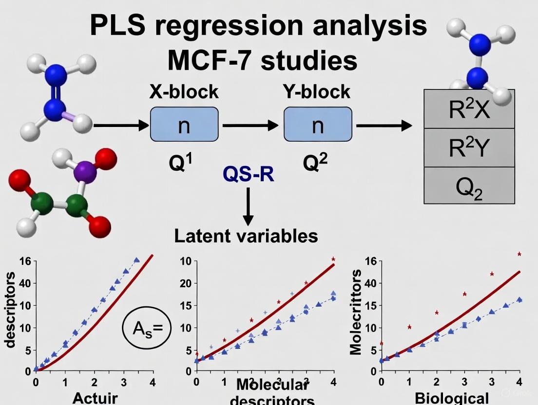
Three-dimensional Quantitative Structure-Activity Relationship (3D-QSAR) modeling represents a powerful computational approach in breast cancer drug discovery, with MCF-7 serving as the primary biological validation system. This methodology quantitatively correlates the three-dimensional molecular structures of compounds with their biological activities against MCF-7 cells, typically measured as half-maximal inhibitory concentration (IC₅₀) values converted to pIC₅₀ (-log IC₅₀) for modeling [3] [4]. The core computational technique employed in these analyses is Partial Least Squares (PLS) regression, which effectively handles the multidimensional nature of 3D molecular descriptors while mitigating issues of collinearity [4].
The typical 3D-QSAR workflow begins with molecular alignment, where compounds are spatially superimposed based on their predicted pharmacophoric features [5]. Subsequently, molecular field descriptors are calculated using either Comparative Molecular Field Analysis (CoMFA) or Comparative Molecular Similarity Indices Analysis (CoMSIA) methodologies [3]. These descriptors capture essential steric, electrostatic, hydrophobic, and hydrogen-bonding properties that influence biological activity. Recent studies have demonstrated robust 3D-QSAR models with high predictive power, including CoMFA (Q² = 0.62, R² = 0.90) and CoMSIA (Q² = 0.71, R² = 0.88) models for tetrahydrobenzo[4,5]thieno[2,3-d]pyrimidine derivatives, validated through external validation (R²ext = 0.90 and R²ext = 0.91, respectively) [3].
The application of these models has successfully identified novel inhibitor candidates with significant binding affinities and robust stabilities, as confirmed through molecular docking, molecular dynamics simulations, and binding free energy calculations [3]. For natural products like maslinic acid analogs, 3D-QSAR modeling has yielded excellent statistical parameters (r² = 0.92, q² = 0.75), enabling virtual screening of potential analogs and identification of compound P-902 as a promising hit against multiple targets including AKR1B10, NR3C1, PTGS2, and HER2 [4].
Diagram 1: 3D-QSAR Workflow with PLS Regression
Advanced Cell Culture Models: 3D Spheroid Systems
Traditional two-dimensional (2D) cell culture models have significant limitations in replicating the physiological microenvironment of solid tumors. To address this, three-dimensional (3D) spheroid culture systems have been developed for MCF-7 cells, creating more clinically relevant models for drug screening [6]. These tumoroids exhibit drug resistance profiles more closely resembling solid tumors, making them particularly valuable for preclinical drug development [6].
A recently developed protocol enables robust MCF-7 spheroid growth using U-bottom, clear, cell-repellent surface 96-well plates [6]. The methodology involves seeding 500-5,000 cells per well in phenol red-free DMEM medium supplemented with 10% FBS, 0.01 mg/ml bovine insulin, 10 nM estradiol, and standard antibiotics [6]. Critical technical aspects include careful medium exchange every two days and minimal disturbance during handling. Under these conditions, MCF-7 cells form single spheroids per well that can be maintained for over 30 days, with spheroid volume increasing over a hundred-fold [6].
Notably, drug sensitivity profiles differ significantly between 2D and 3D cultures. Research using 3D MCF-7 spheroids suggests that estrogen sulfotransferase, steroid sulfatase, and the G protein-coupled estrogen receptor may play critical roles in spheroid growth, while estrogen receptors α and β may have diminished importance in this context [6]. This model system enables more physiologically relevant assessment of compound efficacy and has potential for personalized cancer drug development using patient-derived tumor tissues [6].
Table 2: Experimental Systems for MCF-7 in Drug Discovery
| System Type | Key Features | Applications in Drug Discovery | References |
|---|---|---|---|
| 2D Monolayer Culture | Standard adherent growth; High-throughput capability | Primary compound screening; Mechanism of action studies | [1] |
| 3D Spheroid Culture | Physiologically relevant microenvironment; Gradient conditions | Advanced efficacy assessment; Resistance mechanism studies | [6] |
| Co-culture Systems | Interaction with bystander cells (HSCs, MSCs) | Metastasis and heterogeneity studies; Microenvironment interactions | [2] |
| Computational 3D-QSAR | Structure-activity relationship modeling; Virtual screening | Lead identification and optimization; Activity prediction | [3] [4] |
Experimental Protocols and Methodologies
Standard MCF-7 Cell Culture Protocol
Materials Required:
- MCF-7 human breast cancer cells (ATCC HTB-22)
- Low glucose Dulbecco's Modified Eagle's Medium (DMEM)
- Fetal Bovine Serum (FBS)
- 2 mM glutamine
- 0.01 mg/ml insulin
- 1% penicillin/streptomycin mix
- T75 culture flasks
- Incubator maintained at 37°C with 5% CO₂
Procedure:
- Seed MCF-7 cells in T75 flasks at a density of 1×10⁶ cells/flask in complete medium [1].
- Culture cells in low glucose DMEM supplemented with 10% FBS, 2 mM glutamine, 0.01 mg/ml insulin, and 1% penicillin/streptomycin [1].
- Maintain cultures at 37°C in a humidified atmosphere of 5% CO₂.
- Renew culture medium twice weekly.
- Passage cells weekly at a sub-cultivation ratio of 1:3 using standard trypsinization procedures [1].
3D Spheroid Culture Protocol for Drug Screening
Materials Required:
- U-bottom, clear, cell-repellent surface 96-well plates (e.g., Greiner Bio-One)
- Phenol red-free DMEM medium (Life Technologies)
- Fetal bovine serum (Quality Biological Inc.)
- 100× penicillin/streptomycin solution
- 100× glutamine solution
- 0.01 mg/ml bovine insulin
- 10 nM estradiol
Procedure:
- Expand MCF-7 cells using standard 2D culture conditions to generate sufficient cell numbers [6].
- Prepare single-cell suspension and seed 500-5,000 cells per well in 200 μL of complete medium into U-bottom 96-well plates [6].
- Centrifuge plates at 1000 RPM for 5 minutes to encourage cell aggregation at the well bottom.
- Carefully transfer plates to incubator and maintain at 37°C with 5% CO₂ without disturbance.
- Every two days, carefully remove 150 μL of medium (approximately 75%) using a 200 μL multichannel pipette held at a 90° angle to the well, and replace with fresh pre-warmed medium [6].
- For drug treatment studies, add compounds after each medium change, using appropriate vehicle controls.
- Monitor spheroid growth and morphology regularly using microscopy, measuring spheroid diameter and calculating volume using the formula: V = 4/3πr³.
- Culture can be maintained for over 30 days with careful handling and regular medium exchange [6].
3D-QSAR Model Development Protocol
Materials Required:
- SYBYL-X 2.1 software (Certara) or equivalent molecular modeling platform
- Dataset of compounds with known MCF-7 inhibitory activities (IC₅₀ values)
- Computational resources for molecular dynamics simulations
Procedure:
- Data Preparation: Collect a series of compounds with experimentally determined IC₅₀ values against MCF-7 cells. Convert IC₅₀ to pIC₅₀ (-log IC₅₀) for QSAR analysis [3].
- Molecular Structure Preparation: Build 3D structures of all compounds and optimize geometries using appropriate force fields (e.g., Tripos force field) [3].
- Molecular Alignment: Select the most active compound as template and align all molecules to this template using field-based or feature-based alignment methods [3] [5].
- Descriptor Calculation: Calculate 3D field descriptors using CoMFA (steric and electrostatic fields) and/or CoMSIA (additional hydrophobic, hydrogen bond donor/acceptor fields) [3].
- PLS Model Development: Use Partial Least Squares regression to correlate molecular descriptors with biological activity. Determine optimal number of components using cross-validation [4].
- Model Validation: Validate model using leave-one-out (LOO) cross-validation and external test set validation. Acceptable models should have q² > 0.5 and r² > 0.8 [4] [5].
- Model Application: Use validated model to predict activities of virtual compounds and guide lead optimization efforts.
Diagram 2: Experimental-Digital Workflow Integration
The Scientist's Toolkit: Essential Research Reagents
Table 3: Essential Research Reagents for MCF-7 Studies
| Reagent Category | Specific Examples | Function in Research | References |
|---|---|---|---|
| Cell Culture Media | Low glucose DMEM with phenol red-free option | Supports MCF-7 growth while eliminating estrogenic effects of phenol red | [1] [6] |
| Culture Supplements | Fetal Bovine Serum (10%), Insulin (0.01 mg/mL) | Provides essential growth factors and hormones | [1] [6] |
| Hormone/Inhibitors | 17β-estradiol, Tamoxifen, ICI 182,780 | Modulates estrogen signaling pathways; positive/negative controls | [1] [6] |
| 3D Culture Systems | U-bottom low attachment plates, Extracellular matrix hydrogels | Enables spheroid formation mimicking tumor microenvironment | [6] |
| Viability Assays | MTT, WST-1, Resazurin reduction assays | Quantifies cell viability and compound cytotoxicity | [5] |
| Computational Tools | SYBYL, Forge, Molecular docking software | Enables 3D-QSAR modeling and virtual screening | [3] [4] |
Emerging Applications and Future Directions
The application of MCF-7 cells in drug discovery continues to evolve with emerging technologies. Recent advances include the development of novel nanocarrier systems for targeted drug delivery, such as silver nanoparticle-paclitaxel (AgNPs@PTX) conjugates that demonstrate enhanced cytotoxicity against MCF-7 cells (IC₅₀ = 1.7 μg/mL) compared to single agents [7]. These approaches address limitations of conventional chemotherapy by improving solubility, permeability, and targeted delivery while reducing systemic toxicity.
Another significant advancement involves understanding cellular plasticity in response to microenvironmental signals. Research demonstrates that serotonin (5-HT) signaling can modulate breast cancer cell behavior, promoting aggressive features through downregulation of hormone receptors and HER2, effectively inducing a triple-negative-like phenotype in MCF-7 cells [8]. This phenotypic plasticity underscores the importance of microenvironmental factors in cancer progression and therapeutic response.
The integration of computational predictions with experimental validation represents the most promising future direction. As 3D-QSAR models become increasingly sophisticated through machine learning approaches and more diverse training sets, their predictive accuracy for MCF-7 cytotoxicity continues to improve. These computational tools, combined with physiologically relevant 3D culture models and high-content screening approaches, create a powerful platform for accelerating breast cancer drug discovery and development.
Three-dimensional Quantitative Structure-Activity Relationship (3D-QSAR) represents a pivotal computational methodology in modern ligand-based drug design, enabling researchers to correlate the three-dimensional molecular properties of compounds with their biological activity [9]. In the context of breast cancer research, particularly against the MCF-7 cell line—a well-characterized estrogen receptor alpha (ER-α) positive model derived from human breast adenocarcinoma—3D-QSAR techniques have become indispensable for developing novel therapeutic agents [5]. Unlike traditional QSAR that utilizes computed molecular descriptors, 3D-QSAR methodologies analyze spatial molecular interaction fields, providing visual contours that guide medicinal chemists in optimizing compound structures for enhanced potency [3] [10].
The foundational principle of 3D-QSAR rests on the concept that a compound's biological activity is dependent on its interaction with a specific biological target, mediated through its electrostatic, steric, and hydrophobic properties arranged in three-dimensional space [9]. For breast cancer targets such as aromatase (PDB: 3S7S) or ER-α (PDB: 4XO6), understanding these spatial relationships is crucial for designing effective inhibitors [11] [10]. This application note details the core methodologies of Comparative Molecular Field Analysis (CoMFA) and Comparative Molecular Similarity Indices Analysis (CoMSIA), framed within a Partial Least Squares (PLS) regression analysis context for MCF-7 breast cancer research.
Theoretical Foundations of CoMFA and CoMSIA
Molecular Fields and Interaction Energies
CoMFA (Comparative Molecular Field Analysis) operates on the principle that biological activity correlates with interaction energies between a target receptor and probe atoms positioned around the molecules in a dataset [3] [12]. The methodology computes steric fields using a Lennard-Jones potential function and electrostatic fields using a Coulombic potential function [10]. These fields are calculated at regularly spaced grid points surrounding the aligned molecules, creating a data matrix where each row represents a compound and each column represents the interaction energy at a specific grid point.
CoMSIA (Comparative Molecular Similarity Indices Analysis) extends beyond CoMFA by incorporating additional molecular fields and employing a Gaussian-type distance-dependent function to avoid singularities at molecular surfaces [3] [13]. CoMSIA typically evaluates five similarity indices: steric, electrostatic, hydrophobic, hydrogen bond donor, and hydrogen bond acceptor fields [11] [10]. The inclusion of hydrophobic and explicit hydrogen bonding fields often makes CoMSIA models more interpretable in medicinal chemistry applications, particularly for breast cancer targets where these interactions play crucial roles in ligand-receptor recognition [10].
Alignment Rules and Molecular Superposition
Molecular alignment constitutes the most critical step in both CoMFA and CoMSIA analyses, as the resulting models are highly sensitive to the relative orientation and conformation of the molecules in the dataset [3] [5]. Several alignment strategies are employed in practice:
- Pharmacophore-based alignment: Uses common chemical features identified from active molecules [5].
- Database alignment: Aligns molecules to a predefined template structure, often the most active compound [3] [10].
- Docking-based alignment: Utilizes binding conformations obtained from molecular docking into the target protein's active site [12].
For MCF-7 inhibitors, the selection of appropriate alignment rules must consider the binding mode to relevant targets such as ER-α or aromatase [3] [10]. A robust alignment should place pharmacophoric features in consistent orientations across all molecules in the dataset.
Comparative Analysis of CoMFA and CoMSIA Descriptors
Table 1: Field Descriptors in CoMFA and CoMSIA Methodologies
| Field Type | CoMFA | CoMSIA | Physical Basis | Role in MCF-7 Inhibition |
|---|---|---|---|---|
| Steric | Yes | Yes | Lennard-Jones potential | Optimal bulky groups prevent receptor binding [3] |
| Electrostatic | Yes | Yes | Coulombic potential | Charge complementarity with target [11] |
| Hydrophobic | No | Yes | Hydrophobic interactions | Critical for cell permeability and aromatase binding [10] |
| Hydrogen Bond Donor | No | Yes | Donor ability | Targets receptor H-bond acceptors [5] |
| Hydrogen Bond Acceptor | No | Yes | Acceptor ability | Targets receptor H-bond donors [5] |
Statistical Foundation in PLS Regression
Both CoMFA and CoMSIA utilize Partial Least Squares (PLS) regression to handle the high-dimensional, collinear field data generated during analysis [12] [9]. PLS reduces the original variables (interaction energies at grid points) to a smaller number of latent variables that maximize the covariance between the molecular fields and biological activity [12]. The optimal number of components is determined through cross-validation, typically using the leave-one-out method, to prevent overfitting and ensure model robustness [3] [10].
The statistical quality of 3D-QSAR models is evaluated using several key parameters:
- Q²: Cross-validated correlation coefficient, indicating predictive ability (should be >0.5 for robust models)
- R²: Non-cross-validated correlation coefficient, measuring model fit (should be >0.8)
- R²pred: External validation correlation coefficient, assessing prediction for test set compounds [3] [10]
Table 2: Representative Statistical Parameters from Recent MCF-7 3D-QSAR Studies
| Compound Class | Method | Q² | R² | R²pred | Reference |
|---|---|---|---|---|---|
| Tetrahydrobenzo[4,5]thieno[2,3-d]pyrimidine | CoMFA | 0.62 | 0.90 | 0.90 | [3] |
| Tetrahydrobenzo[4,5]thieno[2,3-d]pyrimidine | CoMSIA | 0.71 | 0.88 | 0.91 | [3] |
| Thioquinazolinone | CoMSIA | 0.669 | 0.989 | 0.936 | [10] |
| Pyrazole-benzimidazole | CoMSIA | N/R | N/R | N/R | [13] |
| 1,4-quinone and quinoline | CoMSIA | N/R | N/R | N/R | [11] |
N/R = Not specifically reported in the search results
Experimental Protocol for 3D-QSAR Model Development
Dataset Preparation and Molecular Modeling
A typical workflow for developing 3D-QSAR models against MCF-7 breast cancer cells involves several methodical steps:
Step 1: Data Collection and Preparation
- Collect a series of compounds with experimentally determined inhibitory activities (IC₅₀ values) against MCF-7 cells [3] [10].
- Convert IC₅₀ values to pIC₅₀ (-logIC₅₀) for use as the dependent variable [3].
- Divide the dataset into training set (typically 70-80% of compounds) for model building and test set (20-30%) for external validation [3] [10].
Step 2: Molecular Structure Optimization
- Sketch molecular structures using modeling software such as SYBYL or Maestro [3] [5].
- Geometry optimization using appropriate force fields (e.g., Tripos force field) with Gasteiger-Hückel partial atomic charges [3] [10].
- Conformational analysis to identify lowest energy conformations or biologically relevant conformers [5].
Step 3: Molecular Alignment
- Select a template molecule, typically the most active compound [3] [10].
- Align all molecules using a consistent rule (pharmacophore-based, database, or docking-based) [5].
- Verify alignment quality through visual inspection and statistical metrics.
Figure 1: 3D-QSAR Model Development Workflow
Field Calculation and PLS Analysis
Step 4: Field Calculation and Data Table Construction
- For CoMFA: Calculate steric and electrostatic fields using a sp³ carbon probe atom with +1 charge on a 2Å grid [3].
- For CoMSIA: Calculate steric, electrostatic, hydrophobic, and hydrogen bond donor/acceptor fields with attenuation factor of 0.3 [3] [10].
- Construct data table with pIC₅₀ values as dependent variable and field values as independent variables.
Step 5: PLS Regression and Model Validation
- Perform PLS regression with cross-validation to determine optimal number of components [3] [12].
- Validate model using external test set to calculate R²pred [3] [10].
- Assess model robustness through various statistical metrics including standard error of estimate and F-value [10].
Research Reagent Solutions for 3D-QSAR
Table 3: Essential Computational Tools for 3D-QSAR Studies
| Tool Category | Specific Software/Resource | Application in 3D-QSAR | Relevance to MCF-7 Research |
|---|---|---|---|
| Molecular Modeling | SYBYL-X (Certara) [3] | Structure building, optimization, CoMFA/CoMSIA | Standard platform for 3D-QSAR development |
| Molecular Modeling | Maestro (Schrödinger) [5] | Pharmacophore modeling, molecular alignment | Phase module for pharmacophore-based alignment |
| Docking Software | AutoDock, GOLD | Binding mode prediction for alignment | Docking-based alignment for protein targets |
| ADMET Prediction | SwissADME, pkCSM | Drug-likeness and toxicity screening | Prioritize compounds with favorable profiles [3] [10] |
| Dynamics Software | GROMACS, AMBER | Molecular dynamics simulations | Validate stability of designed complexes [3] |
Application in Breast Cancer MCF-7 Research: Case Studies
Tetrahydrobenzo[4,5]thieno[2,3-d]pyrimidine Derivatives
A recent study demonstrated the successful application of 3D-QSAR for designing tetrahydrobenzo[4,5]thieno[2,3-d]pyrimidine derivatives as MCF-7 inhibitors [3]. The researchers developed both CoMFA (Q² = 0.62, R² = 0.90) and CoMSIA (Q² = 0.71, R² = 0.88) models with excellent predictive capabilities, confirmed through external validation (R²ext = 0.90 and 0.91 respectively) [3]. The contour maps revealed that:
- Electrostatic fields: Negative charge near specific substituents enhances activity
- Steric fields: Bulky groups at certain positions improve receptor binding
- Hydrophobic fields: Hydrophobic substituents at defined regions increase potency
These insights guided the design of six candidate inhibitors with predicted superior activity, subsequently validated through molecular docking and molecular dynamics simulations targeting ER-α (PDB: 4XO6) [3].
Thioquinazolinone Derivatives as Aromatase Inhibitors
Another study focused on thioquinazolinone derivatives as aromatase inhibitors for breast cancer treatment [10]. The optimal CoMSIA model demonstrated strong statistical values (Q² = 0.669, R² = 0.989, R²pred = 0.936), with field contributions of electrostatic (18.8%), hydrophobic (27.3%), hydrogen bond donor (23.8%), and hydrogen bond acceptor (30.1%) [10]. The contour maps provided specific guidance for molecular modifications:
- Hydrogen bond acceptors: Near specific ring positions crucial for activity
- Hydrophobic groups: At defined molecular regions enhance binding
- Electrostatic properties: Positive potential near substituents improves potency
The study designed new compounds based on these insights and verified their binding modes through molecular docking with aromatase (PDB: 3S7S) [10].
Figure 2: Drug Design Workflow Using 3D-QSAR Results
Advanced Applications and Integration with Other Methods
Multi-Method Validation Approaches
Contemporary 3D-QSAR studies for breast cancer research increasingly integrate multiple computational and experimental approaches to validate findings:
- Molecular Docking: Verifies binding modes suggested by 3D-QSAR contours and identifies key protein-ligand interactions [3] [10].
- Molecular Dynamics Simulations: Assesses complex stability over time (typically 100 ns) and calculates binding free energies using MM/GBSA or MM/PBSA methods [3] [13].
- ADMET Predictions: Evaluates drug-likeness, pharmacokinetic properties, and potential toxicity of designed compounds before synthesis [3] [10].
- Principal Component Analysis (PCA) and Free Energy Landscape (FEL): Provides additional insights into molecular stability and conformational space [13].
This integrated approach ensures that compounds designed using 3D-QSAR guidance not only exhibit predicted high activity but also possess favorable drug-like properties and binding stability, accelerating the discovery of effective MCF-7 inhibitors for breast cancer treatment [3] [13] [10].
Why PLS Regression is the Gold Standard for 3D-QSAR Model Development
Partial Least Squares (PLS) regression stands as the cornerstone statistical method for developing robust three-dimensional quantitative structure-activity relationship (3D-QSAR) models in drug discovery. This protocol details the application of PLS regression within 3D-QSAR frameworks, specifically contextualized for breast cancer research utilizing MCF-7 cell line assays. We provide comprehensive methodologies for building, validating, and interpreting CoMFA and CoMSIA models, including detailed workflows for molecular alignment, descriptor calculation, and model validation. The documented protocols leverage proven applications in designing latrunculin-based actin inhibitors and aromatase-targeting compounds, providing researchers with standardized procedures for implementing this powerful analytical approach in their anti-breast cancer drug development campaigns.
In the field of computer-aided drug design, 3D-QSAR methodologies have emerged as essential tools for correlating the three-dimensional structural properties of compounds with their biological activity. Unlike traditional 2D-QSAR that utilizes molecular descriptors invariant to conformation, 3D-QSAR incorporates spatial and electrostatic properties, providing superior insights into structure-activity relationships [14]. The Comparative Molecular Field Analysis (CoMFA) and Comparative Molecular Similarity Indices Analysis (CoMSIA) represent the most widely adopted 3D-QSAR approaches, generating thousands of highly correlated descriptors from molecular interaction fields [15].
PLS regression serves as the fundamental statistical engine for analyzing these complex descriptor matrices. As a variation of principal component regression, PLS projects the original variables into a smaller set of latent variables that maximize the covariance between predictor and response blocks [12]. This capability makes PLS uniquely suited for 3D-QSAR applications where the number of independent variables (grid points) significantly exceeds the number of observations (compounds) and where substantial multicollinearity exists among descriptors [12] [16]. The robustness of PLS in handling such challenging datasets has established it as the gold standard for 3D-QSAR model development across diverse therapeutic areas, including breast cancer research targeting MCF-7 proliferation pathways.
Theoretical Foundations and Advantages of PLS
Mathematical Principles of PLS Regression
PLS regression operates by simultaneously projecting the variable matrix X (3D-field descriptors) and the response vector Y (biological activities) to new coordinates, maximizing the explained variance in both spaces. The algorithm identifies linear combinations of the original variables (latent variables or components) that successively maximize the covariance between X and Y. This approach differs fundamentally from principal component analysis (PCA), which only considers the variance in the X-space without regard to the response variable [16].
The PLS model can be represented as: X = TP′ + E and Y = UQ′ + F where T and U are the score matrices for X and Y, P and Q are the loading matrices, and E and F are the error terms. The inner relationship between the score vectors is established through U = TD + H, where D is a diagonal matrix and H represents the residuals [16].
Comparative Advantages for 3D-QSAR
Table 1: Key Advantages of PLS Regression in 3D-QSAR
| Advantage | Technical Rationale | Impact on Model Quality |
|---|---|---|
| Handling Multidimensional Descriptors | Capable of analyzing datasets where variables >> samples (e.g., thousands of grid points vs. dozens of compounds) [12] | Enables comprehensive 3D-field analysis without dimensionality reduction |
| Managing Correlated Variables | Effectively handles inter-descriptor correlations inherent in CoMFA/CoMSIA grids [12] | Prevents instability in coefficient estimates |
| Reducing Overfitting Risk | Latent variable selection based on cross-validation minimizes chance correlations [12] [16] | Enhances model predictivity for new chemical entities |
| Integration with Cross-Validation | Compatible with leave-one-out (LOO) and leave-multiple-out (LMO) validation techniques | Provides robust q² metrics for model selection |
The theoretical superiority of PLS for 3D-QSAR was demonstrated in a study of latrunculin-based actin inhibitors, where models developed with PLS regression achieved exceptional statistical quality (q² = 0.621-0.659, r² = 0.938-0.965) [12]. These models successfully predicted the antiproliferative activities against MCF-7 breast cancer cells for an external test set of five compounds, validating the practical utility of the PLS approach.
Experimental Protocols and Methodologies
Comprehensive Workflow for 3D-QSAR with PLS
The following diagram illustrates the standardized workflow for developing validated 3D-QSAR models using PLS regression:
Data Collection and Preparation Protocol
Objective: Assemble a structurally diverse dataset with consistent biological activity data.
- Compound Selection: Curate 20-50 congeneric compounds with measured IC₅₀ values against MCF-7 breast cancer cells [12] [17]. Ensure structural diversity while maintaining a common scaffold to assume similar binding modes.
- Activity Data: Express biological activity as pIC₅₀ (-logIC₅₀) to create a linearly correlated response variable [12]. All activity data should be generated under uniform experimental conditions (e.g., consistent assay protocols, incubation times, and passage numbers for MCF-7 cells).
- Training/Test Sets: Apply Kennard-Stone algorithm or similar approach to divide compounds into training (70-80%) and external test sets (20-30%) [16] [17].
Molecular Modeling and Alignment Protocol
Objective: Generate bioactive conformations and align molecules in 3D space.
- 3D Structure Generation: Convert 2D structures to 3D coordinates using cheminformatics tools (RDKit, OpenBabel) [14].
- Conformation Optimization: Perform geometry optimization using molecular mechanics (UFF, MMFF94s) or semi-empirical quantum mechanical methods (AM1, PM3) [14].
- Molecular Alignment:
- Pharmacophore-Based: For targets with known active site structure (e.g., aromatase in breast cancer), use docking-derived poses from software like AutoDock Vina or GOLD [18] [17].
- Ligand-Based: For targets with unknown structure, employ maximum common substructure (MCS) or field-based alignment methods [14].
- Reference Compound: Select the most active compound or one with confirmed bioactive conformation as alignment template [17].
3D Descriptor Calculation and PLS Implementation
Objective: Calculate molecular interaction fields and build PLS regression models.
- CoMFA Field Calculation:
- CoMSIA Field Calculation:
- Implement same grid parameters as CoMFA
- Calculate similarity indices for steric, electrostatic, hydrophobic, and hydrogen-bond donor/acceptor fields using Gaussian-type distance functions [14]
- PLS Regression Implementation:
- Data Preprocessing: Apply block-scaling to balance steric/electrostatic field contributions and column-wise standardization (unit variance) [14]
- Component Selection: Determine optimal number of latent variables through leave-one-out cross-validation, selecting components where q² is maximized [12]
- Model Fitting: Develop final model using optimal components on entire training set without cross-validation [12]
Model Validation Protocol
Objective: Establish statistical robustness and predictive power of 3D-QSAR models.
- Internal Validation:
- Calculate cross-validated correlation coefficient (q²) using leave-one-out procedure
- Acceptable threshold: q² > 0.5 for predictive models [16]
- Compute non-cross-validated correlation coefficient (r²) and standard error of estimate
- External Validation:
- Robustness Assessment:
Table 2: Statistical Benchmarks for Validated 3D-QSAR Models
| Statistical Parameter | Acceptable Threshold | Excellent Performance | Application in MCF-7 Research |
|---|---|---|---|
| q² (LOO cross-validation) | > 0.5 | > 0.6 | Latrunculin study: q² = 0.621-0.659 [12] |
| r² (non-cross-validated) | > 0.8 | > 0.9 | Latrunculin study: r² = 0.938-0.965 [12] |
| Standard Error of Estimate | Minimized relative to activity range | < 0.3 log units | Critical for predicting antiproliferative potency |
| r²pred (external test set) | > 0.6 | > 0.7 | Successfully predicted 5 external compounds [12] |
| Components | Avoid overfitting | Optimal q² plateau | Typically 4-7 components for CoMFA/CoMSIA |
Research Reagent Solutions for MCF-7 3D-QSAR
Table 3: Essential Research Reagents and Computational Tools
| Category | Specific Tools/Reagents | Function in 3D-QSAR Workflow |
|---|---|---|
| Cell Lines & Assays | MCF-7 (HTB-22) human breast adenocarcinoma cells [12] [19] | Standardized cellular model for determining antiproliferative IC₅₀ values |
| Biological Assays | MTT proliferation assay [12] | Quantification of cell viability and compound cytotoxicity |
| Computational Chemistry | SYBYL [12], Open3DQSAR [18] | Commercial and open-source platforms for CoMFA/CoMSIA analysis |
| Molecular Modeling | RDKit [14], AutoDock Vina [17] | 3D structure generation, optimization, and docking studies |
| Statistical Analysis | PLS implementation in SYBYL [12], scikit-learn (Python) | Core regression algorithm for model development |
| Chemical Libraries | Thiosemicarbazone, 1,2,4-triazole derivatives [17] | Structurally diverse compounds for building robust QSAR models |
Application in Breast Cancer MCF-7 Research
The integration of PLS-based 3D-QSAR models has demonstrated significant impact in anti-breast cancer drug discovery. In a seminal study investigating latrunculin-based actin inhibitors, researchers developed CoMFA and CoMSIA models using PLS regression that accurately predicted antiproliferative activities against MCF-7 cells [12]. The models successfully guided structural optimization by identifying critical steric and electrostatic features contributing to potency, particularly the importance of the C-17 lactol hydroxyl group for interacting with arginine 210 in actin [12].
More recently, PLS-driven 3D-QSAR approaches have been applied to aromatase inhibitors for breast cancer treatment, with studies incorporating both ligand-based and structure-based design elements [17]. These models successfully correlated structural features of thiosemicarbazone and triazole derivatives with aromatase inhibition, providing visual contour maps that guided the design of novel compounds with predicted enhanced activity [17]. The robust statistical foundation provided by PLS regression enabled researchers to confidently prioritize synthetic targets for experimental validation.
Advanced Implementation Strategies
Integration with Docking Studies
Combining 3D-QSAR with molecular docking creates a powerful synergistic approach for drug design. The docking poses provide biologically relevant alignment rules based on protein-ligand interactions, while 3D-QSAR contour maps interpret the resulting models in chemical terms [18] [17]. This combined methodology was successfully applied in designing TRPV1 channel antagonists, where docking into the cryo-EM structure (PDB: 8GFA) provided the alignment for subsequent CoMFA analysis [18].
Handling Alignment-Sensitive Scenarios
Molecular alignment remains the most critical step in traditional CoMFA implementations. When dealing with structurally diverse datasets, consider these advanced approaches:
- Docking-Based Alignment: Use consensus docking poses from multiple algorithms to establish alignment rules [17]
- Field-Based Alignment: Implement field-fit techniques that optimize superposition based on similarity of molecular fields rather than atom positions [14]
- Multiple Conformation Approaches: Incorporate several low-energy conformations per compound to account for flexibility [18]
Troubleshooting and Quality Control
Issue: Low q² despite high r²
- Potential Cause: Overfitting due to excessive latent variables
- Solution: Re-evaluate optimal component number using cross-validation; consider bootstrapping for more robust component selection
Issue: Poor external prediction accuracy
- Potential Cause: Test compounds outside applicability domain of training set
- Solution: Implement applicability domain assessment using leverage and standardization approaches; expand structural diversity of training set
Issue: Inconsistent contour map interpretation
- Potential Cause: Suboptimal alignment of molecules with divergent binding modes
- Solution: Validate alignment strategy with known crystal structures or through docking studies; consider receptor-based alignment when protein structure available
PLS regression has firmly established itself as the statistical foundation for 3D-QSAR model development due to its unique ability to handle the high-dimensional, multicollinear datasets generated by CoMFA and CoMSIA methodologies. The protocols outlined in this document provide researchers with a comprehensive framework for implementing PLS-based 3D-QSAR in breast cancer drug discovery, with specific application to MCF-7 targeted therapies. Through proper implementation of alignment strategies, descriptor calculation, and validation protocols, researchers can develop robust predictive models that significantly accelerate the design and optimization of novel anti-breast cancer agents. The continued integration of these approaches with structural biology and machine learning techniques promises to further enhance their predictive power and utility in drug development campaigns.
In the field of computational drug design, particularly in the development of therapeutics for breast cancer, Partial Least Squares (PLS) regression serves as the statistical backbone for Three-Dimensional Quantitative Structure-Activity Relationship (3D-QSAR) models. These models connect the molecular features of compounds to their biological activity against specific targets, such as the MCF-7 breast cancer cell line. The reliability of these models is paramount, as they guide the synthesis and testing of new drug candidates. Evaluating this reliability hinges on understanding key statistical metrics: the coefficient of determination (R²) for explanatory power and the predictive squared correlation coefficient (Q²) for predictive capability. A robust 3D-QSAR model must demonstrate high values for both R² and Q², indicating it not only fits the training data well but can also accurately predict the activity of novel compounds, thereby accelerating the discovery of effective anti-cancer agents [20] [3].
Core Statistical Metrics: Definitions and Interpretations
The Coefficient of Determination (R²)
R², or the coefficient of determination, is a fundamental metric that quantifies the goodness-of-fit of a regression model. It measures the proportion of the variance in the dependent variable (e.g., biological activity pIC₅₀) that is predictable from the independent variables (e.g., 3D molecular field descriptors) [21] [22].
Mathematical Definition: R² is calculated as 1 minus the ratio of the residual sum of squares (RSS) to the total sum of squares (TSS). ( R^2 = 1 - \frac{RSS}{TSS} = 1 - \frac{\sum(yi - \hat{y}i)^2}{\sum(yi - \bar{y})^2} ) Where ( yi ) is the observed value, ( \hat{y}_i ) is the predicted value, and ( \bar{y} ) is the mean of observed values [20] [22].
Interpretation: R² values range from 0 to 1. An R² of 1 indicates the model explains all the variability of the response data around its mean, while an R² of 0 indicates the model explains none of the variability. In 3D-QSAR studies for MCF-7, a high R² signifies that the molecular descriptors effectively capture the structural features responsible for biological activity [23] [21].
The Predictive Squared Correlation Coefficient (Q²)
Q², often referred to as the goodness of prediction, is a metric derived from cross-validation that assesses the predictive power of a model on new, unseen data [20].
Mathematical Definition: Q² is calculated as 1 minus the ratio of the predictive residual sum of squares (PRESS) to the total sum of squares (TSS). ( Q^2 = 1 - \frac{PRESS}{TSS} = 1 - \frac{\sum(yi - \hat{y}{i, PRESS})^2}{\sum(yi - \bar{y})^2} ) Where ( \hat{y}{i, PRESS} ) is the predicted value for the i-th observation when the model is built without it (as in Leave-One-Out cross-validation) [20].
Interpretation: Like R², Q² ranges from 0 to 1, though it can be negative if the model predictions are worse than simply using the mean activity. A high Q² value is critical in 3D-QSAR, as it confirms the model's utility in predicting the activity of newly designed compounds before they are synthesized and tested biologically [20] [3].
Comparative Analysis of R² and Q²
The critical distinction between R² and Q² lies in their evaluation of model performance: R² measures fit to existing data, while Q² measures prediction of new data [20]. In practice, a model's R² is always higher than its Q². A large gap between R² and Q² often indicates overfitting, where the model is too complex and describes noise in the training data rather than the underlying relationship. A robust and predictive model is characterized by high values for both R² and Q², with the difference between them being minimal [20] [24].
Table 1: Comparative Overview of R² and Q² in PLS-based 3D-QSAR
| Metric | Evaluates | Calculation Basis | Interpretation in 3D-QSAR |
|---|---|---|---|
| R² (Goodness-of-Fit) | Model's fit to training data | Residual Sum of Squares (RSS) | How well the model explains the activity of the training set compounds. |
| Q² (Goodness-of-Prediction) | Model's predictive ability | Predictive Residual Sum of Squares (PRESS) | How well the model predicts the activity of a external test set or new compounds. |
Application in Breast Cancer MCF-7 Research: A Quantitative Review
The application of R² and Q² in validating 3D-QSAR models for MCF-7 breast cancer research is well-documented in recent literature. The following table summarizes quantitative data from key studies, demonstrating the role of these metrics in practice.
Table 2: Summary of R² and Q² Values from Recent 3D-QSAR Studies on MCF-7 Inhibitors
| Study Compound / Class | Model Type | R² (Training) | Q² (Validation) | External Validation (R²pred) | Reference |
|---|---|---|---|---|---|
| Tetrahydrobenzo[4,5]thieno[2,3-d]pyrimidine derivatives | CoMFA | 0.90 | 0.62 | 0.90 | [3] |
| Tetrahydrobenzo[4,5]thieno[2,3-d]pyrimidine derivatives | CoMSIA | 0.88 | 0.71 | 0.91 | [3] |
| Maslinic acid analogs | PLS Regression | 0.92 | 0.75 | Not Specified | [24] [25] |
| Thioquinazolinone derivatives | CoMSIA | Significant values reported | Significant values reported | Significant ( R^2_{pred} ) reported | [10] |
Interpretation of Case Studies:
- The studies on tetrahydrobenzo[4,5]thieno[2,3-d]pyrimidine derivatives showcase robust and predictive models. The CoMSIA model, for instance, with an R² of 0.88 and a Q² of 0.71, demonstrates a strong balance between explanation and prediction. The high external validation correlation coefficient (R²pred of 0.91) further confirms the model's utility for screening new potential inhibitors [3].
- The Maslinic acid analogs study presents a high R² (0.92) and a strong Q² (0.75), indicating an excellent model. This LOO-validated PLS model was successfully used to screen a large compound library, leading to the identification of a best hit, compound P-902, for further investigation [24] [25].
- These examples underscore that a Q² value above 0.5 is generally considered indicative of a predictive model in chemometrics and QSAR studies, while R² values above 0.8 or 0.9 reflect a strong explanatory model [3] [24].
Experimental Protocols for Model Validation
Protocol 1: Standard Procedure for PLS-based 3D-QSAR Model Development and Validation
This protocol outlines the key steps for building and validating a 3D-QSAR model using PLS regression, ensuring reliable R² and Q² metrics.
Dataset Preparation and Curation
- Activity Data: Collect experimental biological data (e.g., IC₅₀) for a series of compounds against the MCF-7 cell line. Convert IC₅₀ values to pIC₅₀ (pIC₅₀ = -logIC₅₀) for use as the dependent variable [3].
- Data Splitting: Randomly divide the dataset into a training set (typically ~80%) for model building and a test set (the remaining ~20%) for external validation. The test set must be kept blind during model development [3] [10].
Molecular Modeling and Alignment
- Structure Construction: Sketch or build the 3D structures of all compounds using molecular modeling software (e.g., SYBYL-X) [3] [10].
- Geometry Optimization: Minimize the energy of each molecule using a specified force field (e.g., Tripos force field) and assign partial atomic charges (e.g., Gasteiger-Hückel) [3].
- Molecular Alignment: Align all molecules onto a common template, typically the most active or a hypothesized most rigid molecule, using a method like the
distillmodule in SYBYL. This is a critical step for the meaningful calculation of 3D descriptors [3] [10].
Descriptor Calculation and PLS Regression
- Field Calculation: Calculate 3D molecular field descriptors. For CoMFA, compute steric (Lennard-Jones) and electrostatic (Coulombic) fields. For CoMSIA, additional fields like hydrophobic, hydrogen-bond donor, and acceptor may be used [3] [10].
- Model Building: Subject the field descriptors to PLS regression to derive the QSAR model, relating the molecular fields to the biological activity (pIC₅₀).
Internal Validation and Q² Calculation
- Leave-One-Out (LOO) Cross-Validation: Systematically remove one compound from the training set, build the model with the remaining compounds, and predict the activity of the removed compound. Repeat for every compound in the training set [24].
- Calculate Q²: Compute PRESS from the prediction errors during LOO and then calculate Q² using the formula in Section 2.2 [20] [24].
External Validation and Model Application
- Predict Test Set: Use the final model, built on the entire training set, to predict the activities of the blinded test set compounds.
- Calculate R²pred: Calculate the predictive R² (R²pred) for the test set to externally validate the model's power [3] [10].
- Design New Compounds: Utilize the model's contour maps to guide the design of new compounds with predicted high activity. Synthesize and test these compounds to experimentally validate the model's predictions [3].
Protocol 2: Statistical Significance Testing for R² and Q²
This protocol ensures the statistical robustness of the reported metrics.
- Permutation Testing: To confirm the model is not based on chance correlation, repeat the model building process multiple times (e.g., 100 times) with randomly shuffled activity data (Y-scrambling). The R² and Q² of the true model should be significantly higher than those from the scrambled models [10].
- Assessment of Difference (R² - Q²): A small difference (e.g., < 0.3) between R² and Q² generally indicates a robust model without severe overfitting. A larger gap warrants investigation into model complexity or data overfitting [20] [24].
- Bootstrapping: Perform bootstrapping analysis (repeated sampling with replacement from the training set) to estimate the confidence intervals for the PLS regression coefficients and the R²/Q² metrics, providing a measure of their stability [22].
Workflow and Signaling Pathways
The following diagram illustrates the integrated workflow for 3D-QSAR model development and validation, highlighting the roles of R² and Q² at key stages.
The Scientist's Toolkit: Essential Research Reagents and Materials
Table 3: Key Software and Computational Tools for 3D-QSAR Analysis
| Item Name | Function / Application | Relevance to R²/Q² |
|---|---|---|
| SYBYL-X Software | A comprehensive molecular modeling environment used for structure building, energy minimization, molecular alignment, and CoMFA/CoMSIA analysis. | Provides the platform for generating the PLS regression models and automatically calculates R² and Q² during analysis [3] [10]. |
| Leave-One-Out (LOO) Cross-Validation Algorithm | A resampling procedure used to estimate the predictive performance of a model. | This algorithm is the standard method for generating the PRESS statistic, which is required for the calculation of Q² [20] [24]. |
| Training and Test Sets | A curated dataset of compounds with known biological activity, split into subsets for model building and validation. | The training set is used to calculate R². The test set is held back for external validation, providing the final, most rigorous test of predictive power (R²pred) [3] [10]. |
| PLS Regression Algorithm | A statistical method that projects predicted variables and observable variables to a new space, ideal for handling correlated descriptors in QSAR. | The core algorithm that establishes the relationship between molecular structures and activity. It directly generates the model statistics, including R² [20] [26]. |
This application note details a computational protocol for developing and validating a three-dimensional Quantitative Structure-Activity Relationship (3D-QSAR) model. The model is designed to predict the anticancer activity of tetrahydrobenzo[4,5]thieno[2,3-d]pyrimidine derivatives against the MCF-7 breast cancer cell line. The workflow integrates Comparative Molecular Field Analysis (CoMFA) and Comparative Molecular Similarity Indices Analysis (CoMSIA) with Partial Least Squares (PLS) regression to elucidate critical structural features governing biological activity. This provides a rational basis for designing novel, potent inhibitors [3] [27].
Breast cancer, particularly the MCF-7 cell line, represents a major focus in oncology research. The tetrahydrobenzo[4,5]thieno[2,3-d]pyrimidine scaffold has been identified as a promising core structure due to its diverse biological activities, including significant antitumor properties. This scaffold is a bioisostere of quinazoline and has been used as a central framework in developing compounds that potentially inhibit cancer cell proliferation [3].
The primary objective of this case study is to establish a predictive 3D-QSAR model. This model links the three-dimensional molecular properties of a series of derivatives to their half-maximal inhibitory concentration (IC₅₀) against MCF-7 cells. The resulting model serves as a valuable tool for in silico screening and optimization of new candidate molecules before costly synthetic and biological testing [3].
Experimental Protocol and Workflow
Dataset Curation and Preparation
- Data Source: A dataset of 29 tetrahydrobenzo[4,5]thieno[2,3-d]pyrimidine derivatives with known experimental IC₅₀ values against the MCF-7 cell line was compiled from published literature [3].
- Activity Conversion: IC₅₀ values (in molar units) were converted to pIC₅₀ using the formula pIC₅₀ = -log(IC₅₀), which serves as the dependent variable in the QSAR model [3].
- Dataset Division: The dataset was randomly partitioned into a training set (24 compounds) for model development and a test set (5 compounds) for external validation of the model's predictive power [3].
- Structure Preparation: All molecular structures were sketched in 2D and converted into 3D models. Energy minimization was performed using the Tripos force field with Gasteiger-Hückel partial atomic charges in SYBYL-X.2.1 software to obtain stable, low-energy conformations [3].
Molecular Alignment
Molecular alignment is a critical step in 3D-QSAR. The most active compound in the series (3z, pIC₅₀ = 7.0) was selected as the template structure. All other molecules in the dataset were aligned to this template based on their common core structure using the "distill" module in SYBYL 2.1 software to ensure a consistent frame of reference for field calculations [3].
3D-QSAR Model Development and PLS Regression
- Descriptor Calculation: The aligned molecules were placed within a 3D grid. The CoMFA and CoMSIA fields were calculated at each grid point.
- PLS Regression Analysis: The relationship between the calculated molecular field descriptors (independent variables) and the pIC₅₀ values (dependent variable) was modeled using the Partial Least Squares (PLS) algorithm. This technique is ideal for handling data where the number of variables exceeds the number of observations and where variables are highly correlated [3] [4]. The model's complexity (number of latent variables) was optimized to avoid overfitting.
Model Validation
The robustness and predictive ability of the 3D-QSAR models were rigorously assessed using the following methods [3]:
- Internal Validation: Leave-One-Out (LOO) cross-validation was performed on the training set, yielding cross-validated correlation coefficients (Q²).
- External Validation: The model's predictive power was tested by predicting the activity of the five compounds in the external test set that were not used in model building.
- Statistical Metrics: The quality of the model was evaluated using the non-cross-validated correlation coefficient (R²) and standard error of estimate.
The following workflow diagram illustrates the key stages of the 3D-QSAR modeling process.
Key Results and Model Statistics
The established 3D-QSAR models demonstrated high statistical quality and robust predictive ability, as summarized in the table below.
Table 1: Statistical Parameters of the Developed 3D-QSAR Models [3]
| Model | Cross-Validated Correlation Coefficient (Q²) | Non-Cross-Validated Correlation Coefficient (R²) | Number of Components | Standard Error of Estimate | External Validation Correlation (R²ext) |
|---|---|---|---|---|---|
| CoMFA | 0.62 | 0.90 | 6 | 0.28 | 0.90 |
| CoMSIA | 0.71 | 0.88 | 6 | 0.31 | 0.91 |
The contour maps generated from the models provide visual guidance for molecular design. For example:
- CoMFA Steric Fields: Green contours near a specific substituent position indicate regions where bulky groups enhance activity, while yellow contours show where bulky groups are detrimental.
- CoMFA Electrostatic Fields: Blue contours indicate regions where electropositive groups are favorable, whereas red contours show where electronegative groups boost activity [3].
The Scientist's Toolkit: Essential Research Reagents and Software
Table 2: Key Research Reagents and Computational Tools for 3D-QSAR
| Item Name / Software | Function in the Protocol | Specific Example / Note |
|---|---|---|
| SYBYL-X | Integrated software suite for molecular modeling, structure building, alignment, and 3D-QSAR analysis. | Used for energy minimization (Tripos force field), molecular alignment (distill module), and CoMFA/CoMSIA calculations [3]. |
| PLS Regression | Core statistical algorithm used to correlate 3D molecular field descriptors with biological activity. | Implemented within SYBYL; optimal number of components is critical to avoid model overfitting [3] [4]. |
| Tetrahydrobenzo[4,5]thieno[2,3-d]pyrimidine core | The central chemical scaffold upon which derivatives are designed and synthesized. | Acts as a bioisostere for quinazoline; known for antitumor, antimicrobial, and antiviral activities [3]. |
| MCF-7 Cell Line Assay | In vitro biological assay to determine the potency (IC₅₀) of compounds against breast cancer. | Provides the experimental activity data (pIC₅₀) used as the dependent variable for building the QSAR model [3]. |
| Molecular Dynamics (MD) Simulation | Advanced simulation technique to study the stability and dynamics of protein-ligand complexes over time. | Used in subsequent studies (e.g., 100 ns simulations) to validate docking poses and binding stability [3] [28]. |
| ADMET Prediction Tools | In silico software to predict Absorption, Distribution, Metabolism, Excretion, and Toxicity. | Used to evaluate the drug-likeness and pharmacokinetic properties of newly designed compounds before synthesis [3] [4]. |
Advanced Applications and Protocol Extension
The validated 3D-QSAR model is not an endpoint but a starting point for a more comprehensive drug discovery campaign.
Virtual Screening and Molecular Design
The model can be used to screen virtual libraries of compounds by predicting their pIC₅₀ values. Furthermore, the 3D contour maps provide a clear guide for rational drug design:
- To increase potency, introduce substituents that match the favorable steric (green) and electrostatic (blue/red) regions indicated by the model.
- To avoid reducing potency, eliminate groups that fall into unfavorable (yellow) regions [3].
Integration with Molecular Docking
To understand the binding mode of these derivatives, molecular docking was performed against the estrogen receptor alpha (ERα) crystal structure (PDB code: 4XO6). Docking studies help visualize key interactions, such as hydrogen bonds and hydrophobic contacts, between the ligand and the active site of the protein, providing a structural basis for the observed activity [3].
Binding Stability Assessment using MM/GBSA and MD
The binding affinities predicted by docking can be refined using the Molecular Mechanics/Generalized Born Surface Area (MM/GBSA) method to calculate binding free energies. Subsequently, Molecular Dynamics (MD) simulations (e.g., for 100 ns) can be run to assess the stability of the protein-ligand complex under dynamic, physiological-like conditions and to confirm that the binding pose is maintained over time [3] [28].
The relationship between these advanced techniques is summarized in the following workflow.
A Step-by-Step Workflow: Building and Applying Your 3D-QSAR Model with PLS
The development of robust 3D-QSAR models for breast cancer MCF-7 research hinges critically on two preliminary computational procedures: rigorous dataset curation and precise molecular alignment. These foundational steps determine the quality of the molecular descriptors fed into Partial Least Squares (PLS) regression analysis, ultimately governing the predictive power and reliability of the resulting models [9] [17]. In the context of anti-breast cancer drug discovery, these protocols ensure that computational predictions regarding compound activity against MCF-7 cell lines translate effectively to experimental validation, thereby accelerating the identification of promising therapeutic candidates [29].
Dataset Curation Protocol
Data Collection and Standardization
The initial phase involves assembling a structurally diverse yet mechanistically consistent set of compounds with experimentally determined activities against MCF-7 breast cancer cell lines.
- Data Sourcing: Retrieve biological activity data (typically IC50 values) from reliable public databases such as the NPACT database , which specializes in naturally occurring plant-derived anticancer compounds with associated cell line activities [29]. The MCF-7 human breast cancer cell line is frequently used as a model system in such studies [29].
- Activity Value Standardization: Convert concentration values (e.g., IC50 in µM) to a uniform negative logarithmic scale (pIC50) using the formula: pIC50 = -log10(IC50 × 10⁻⁶) [30]. This transformation linearizes the relationship between concentration and biological response for subsequent PLS regression analysis.
- Structure Standardization: Curate and standardize all molecular structures by:
Data Pretreatment and Division
- Descriptor Calculation and Filtering: Calculate molecular descriptors using software such as PaDEL Descriptor. Subsequently, preprocess the generated descriptor matrix to remove constants and near-constant values, reducing noise and computational burden [30].
- Dataset Division: Partition the curated dataset into training and test sets using algorithms such as the Kennard-Stone method. This approach ensures the training set spans the entire chemical space of the dataset, while the test set provides a robust external validation cohort [30]. A typical split allocates approximately 70-80% of compounds for training and 20-30% for testing [29] [30].
Table 1: Key Validation Parameters for Robust QSAR Models
| Parameter | Category | Acceptance Threshold | Purpose |
|---|---|---|---|
| R² | Internal Validation | > 0.6 | Measures goodness-of-fit of the model [29]. |
| Q²loo | Internal Validation | > 0.5 | Evaluates model robustness via leave-one-out cross-validation [29]. |
| R²pred | External Validation | > 0.5 | Assesses predictive power on an external test set [30]. |
| CCC | External Validation | > 0.8 | Concordance Correlation Coefficient; measures agreement between observed and predicted values [29]. |
The following workflow outlines the complete dataset curation and model building process, highlighting the initial critical steps.
Molecular Alignment Strategies
Molecular alignment, the process of superimposing molecules in 3D space based on a common reference framework, is a critical step for 3D-QSAR techniques like CoMFA and CoMSIA. The chosen strategy directly influences the contour maps and the subsequent interpretation of structural features affecting activity [11] [17].
Common Alignment Methodologies
- Pharmacophore-Based Alignment: This method aligns molecules based on common pharmacophoric features (e.g., hydrogen bond donors/acceptors, hydrophobic regions, aromatic rings) believed to be essential for interaction with the biological target [9].
- Database Alignment: A common practice involves using a pre-defined template or a selected active molecule from the dataset as a reference for alignment. For instance, a high-activity compound (e.g., "molecule 4" in one study) is chosen, and all other structures are aligned onto its scaffold to ensure consistency [17].
- Ligand-Based Alignment (Common Substructure): Molecules are superimposed based on a shared common substructure or scaffold. This is particularly effective for congeneric series of derivatives, such as thiosemicarbazone or imidazol-5-ones, where a core structure is maintained [17] [30].
Practical Alignment Protocol
- Template Selection: Identify and energy-minimize the most active compound or a representative template molecule from the dataset using computational methods (e.g., Density Functional Theory (DFT) at the B3LYP/6-31G* level is commonly used for geometric optimization) [30].
- Structural Preparation: Prepare all molecules in the dataset by generating low-energy 3D conformations. It is crucial to consider the biologically active conformation if known.
- Superimposition: Align all molecules onto the selected template based on the chosen strategy (common substructure or pharmacophore points). Software like Spartan or functionality within 3D-QSAR packages (e.g., SYBYL) is typically used for this step [11] [30].
- Validation: Visually inspect the alignment to ensure meaningful overlap of critical functional groups. A poor alignment will lead to statistically insignificant or uninterpretable 3D-QSAR models.
The alignment process establishes the common frame of reference necessary for extracting comparative molecular field descriptors.
The Scientist's Toolkit: Essential Research Reagents & Software
Table 2: Key Software Tools for Dataset Curation and Molecular Alignment
| Tool Name | Category | Primary Function in Protocol |
|---|---|---|
| NPACT Database | Database | Source of curated natural products with anti-MCF-7 activity data [29]. |
| PubChem/ChemSpider | Database | Repositories for retrieving standardized molecular structures [29]. |
| PaDEL-Descriptor | Descriptor Calculator | Calculates molecular descriptors from chemical structures for QSAR [29] [30]. |
| Spartan | Molecular Modeling | Used for quantum mechanical geometry optimization of molecules prior to alignment and descriptor calculation [30]. |
| ChemDraw | Chemical Drawing | Creates and converts 2D chemical structures to 3D formats for further processing [30]. |
| SYBYL (CoMFA/CoMSIA) | 3D-QSAR Platform | Performs molecular alignment, field calculation, and PLS regression analysis to build the 3D-QSAR models [11] [17]. |
| Data Pre-treatment GUI | Data Preprocessing | Removes constant and redundant descriptors to improve model quality and stability [30]. |
In modern computer-aided drug design (CADD), the ability to quantify and model the three-dimensional interactions between a potential drug molecule and its biological target is paramount [31]. Molecular field descriptors are computational representations that numerically capture key aspects of a molecule's shape and interaction potential, providing a cornerstone for Three-Dimensional Quantitative Structure-Activity Relationship (3D-QSAR) studies [14]. These methodologies are particularly vital in targeted cancer therapy research, such as in the discovery of novel anti-proliferative agents against the MCF-7 breast cancer cell line [13] [4]. By correlating these calculated molecular fields with experimentally determined biological activity, researchers can build predictive models that guide the rational design of more potent and selective drug candidates. This application note details the protocols for calculating steric, electrostatic, and hydrophobic field descriptors and their subsequent processing via Partial Least Squares (PLS) regression analysis, framing the discussion within the critical context of breast cancer drug discovery.
Molecular Field Descriptors: Core Concepts and Calculations
Molecular field descriptors map a molecule's spatial interaction properties by probing its 3D structure. The table below summarizes the three primary fields used in 3D-QSAR.
Table 1: Core Molecular Field Descriptors in 3D-QSAR
| Field Type | Physical Significance | Probe Atom/Group | Representation in Contour Maps |
|---|---|---|---|
| Steric | Molecular bulk and van der Waals repulsion/attraction [32] [14]. | sp³ Carbon atom [33] [14]. | Green: Favorable bulky groupsYellow: Unfavorable bulky groups [14]. |
| Electrostatic | Local positive or negative electrostatic potential [32] [14]. | Charged atom (e.g., H⁺ with +1 charge) [33] [14]. | Blue: Favorable positive chargeRed: Favorable negative charge [14]. |
| Hydrophobic | Propensity for hydrophobic interactions [14] [4]. | Hypothetical hydrophobic probe [14]. | Yellow: Favorable hydrophobic groupsWhite: Unfavorable hydrophobic groups. |
These descriptors form the basis of established 3D-QSAR methodologies like Comparative Molecular Field Analysis (CoMFA) and Comparative Molecular Similarity Indices Analysis (CoMSIA) [33] [14]. While CoMFA classically calculates steric (Lennard-Jones) and electrostatic (Coulombic) potentials on a 3D lattice, CoMSIA extends this by using Gaussian-type functions to evaluate steric, electrostatic, hydrophobic, and hydrogen-bonding fields, which often produces more interpretable models and is less sensitive to minor molecular misalignments [14].
Experimental Protocol: Calculation Workflow
The following section provides a detailed, step-by-step protocol for calculating molecular field descriptors and building a 3D-QSAR model with PLS regression, contextualized for a study on MCF-7 breast cancer cell inhibitors [13] [4].
Data Collection and Preparation
- Activity Data: Assemble a congeneric series of compounds with experimentally determined biological activities (e.g., IC₅₀ or MIC values) against the MCF-7 cell line [14] [4]. All data must be acquired under uniform experimental conditions to minimize noise and bias.
- Dataset Division: Divide the dataset into a training set (typically ~80%) for model construction and a test set (typically ~20%) for external validation of the model's predictive power [33] [4].
- Structure Preparation: Convert 2D molecular structures into 3D formats using cheminformatics tools like ChemBio3D [4] or RDKit [14]. Geometry-optimize the 3D structures using molecular mechanics (e.g., Tripos force field, UFF) or quantum mechanical methods to achieve a realistic, low-energy conformation [33] [14].
Molecular Alignment
Molecular alignment is a critical step that assumes all compounds share a similar binding mode to the target.
- Method Selection: Use a common substructure for rigid alignment or a flexible alignment algorithm [14] [34].
- Protocol: In software such as SYBYL-X or Forge, align all molecules onto a chosen template, often the most active compound in the series, based on their maximum common substructure (MCS) or a pre-defined pharmacophore [14] [34]. This ensures all molecules are placed in a common 3D coordinate system.
Field Descriptor Calculation
With aligned molecules, calculate the field descriptors within a defined 3D grid that encompasses all molecules.
- Grid Setup: Create a 3D grid with a spacing of 1.0 or 2.0 Å extending beyond the dimensions of all aligned molecules [33].
- Descriptor Generation:
- For CoMFA: At each grid point, calculate steric (Lennard-Jones potential) and electrostatic (Coulomb potential) interaction energies using a probe atom [33] [14].
- For CoMSIA: Calculate similarity indices for steric, electrostatic, and hydrophobic fields using a Gaussian function at each grid point [14]. A sp³ carbon atom with a +1 charge is a typical probe [33].
- Energy Truncation: Set reasonable cutoffs (e.g., 30 kcal/mol) for steric and electrostatic energies to prevent singularities and improve model stability [33].
The workflow from data preparation to model building is visualized in the following diagram.
Model Building with PLS Regression
The generated field descriptors serve as the independent variables (X-matrix), while the biological activity (e.g., pIC₅₀ = -logIC₅₀) is the dependent variable (Y-matrix) [33] [4].
- Rationale for PLS: PLS regression is the standard method for 3D-QSAR as it effectively handles the high dimensionality and multicollinearity inherent in the descriptor matrix (where the number of grid points far exceeds the number of compounds) [35] [14].
- Protocol Execution:
- Software: Use the PLS module in 3D-QSAR software like SYBYL-X [33] or Forge [4].
- Leave-One-Out (LOO) Cross-Validation: Perform LOO cross-validation on the training set to determine the optimal number of latent variables (also called principal components) that maximizes the cross-validated correlation coefficient (Q²) and minimizes overfitting [33] [4]. A Q² > 0.5 is generally considered acceptable [33].
- Final Model Construction: Using the optimal number of components, build the final PLS model on the entire training set to obtain the conventional correlation coefficient (R²) and standard error of estimate (SEE) [33].
Model Validation and Interpretation
- Validation: Assess the model's predictive power by predicting the activity of the external test set. A predictive correlation coefficient (R²ₚᵣₑ𝒹) greater than 0.6 indicates a robust model [33].
- Interpretation via Contour Maps: The PLS model coefficients are visualized as 3D contour maps around a reference molecule [14]. These maps highlight regions where specific molecular fields are favorably or unfavorably linked with biological activity, providing clear, visual guidance for medicinal chemists to design improved analogs [14] [4].
The Scientist's Toolkit: Essential Research Reagents and Software
Table 2: Key Research Reagents and Computational Tools for 3D-QSAR
| Category / Item | Specific Examples | Function / Application in 3D-QSAR |
|---|---|---|
| Software Suites | SYBYL-X [33], Forge (Cresset) [4], Discovery Studio [34] | Integrated platforms for molecular modeling, alignment, field calculation, and PLS analysis. |
| Cheminformatics Libraries | RDKit [14], ChemBio3D [4] | Open-source and commercial tools for 2D to 3D structure conversion and molecular manipulation. |
| Statistical & ML Libraries | Scikit-learn (Python) [36] | Provides PLSRegression class and other tools for model building and validation outside specialized suites. |
| Target & Compound Data | MCF-7 Breast Cancer Cell Line Assays [13] [4] | Provides essential experimental biological activity data (e.g., IC₅₀) for model training and validation. |
| Chemical Databases | ZINC Database [4] | Publicly accessible database of commercially available compounds for virtual screening of new drug candidates. |
Application in MCF-7 Breast Cancer Research
The integration of these protocols in MCF-7 research is demonstrated in a study on Maslinic acid analogs, where a field-based 3D-QSAR model was developed [4]. The study used the FieldTemplater module in Forge to generate a pharmacophore hypothesis from active compounds, which then guided molecular alignment. The derived PLS regression model showed excellent statistical quality (r² = 0.92, q² = 0.75), validating its predictive capability [4]. The resulting contour maps provided actionable insights, identifying key structural regions where steric bulk and electrostatic groups influence anti-proliferative activity, which were successfully used for the virtual screening and identification of a promising new hit compound, P-902 [4].
Similarly, a study on pyrazole-benzimidazole derivatives targeting MCF-7 cells highlighted the critical roles of electrostatic and hydrophobic fields in inhibiting cancer cell growth. The validated CoMSIA model offered a reliable foundation for designing and predicting the biological effects of new, potent inhibitors [13].
Executing PLS Regression Analysis to Correlate Structure with pIC50 Activity
In the field of breast cancer drug discovery, particularly research targeting the MCF-7 cell line, Three-Dimensional Quantitative Structure-Activity Relationship (3D-QSAR) modeling serves as a crucial computational approach for understanding how structural features of molecules influence their biological activity. Partial Least Squares (PLS) regression represents the statistical cornerstone of these models, enabling researchers to correlate complex 3D molecular descriptors with experimentally determined inhibitory concentrations (pIC50 values). This methodology has been successfully applied to diverse compound classes investigated for anti-cancer activity against MCF-7 breast cancer cells, including latrunculin derivatives [12], maslinic acid analogs [37], benzoxazole derivatives [38], and tetrahydrobenzo[4,5]thieno[2,3-d]pyrimidine derivatives [39]. The primary objective of applying PLS regression in this context is to derive a predictive model that can guide the rational design of novel, more potent therapeutic agents by identifying critical structural regions that enhance or diminish anticancer activity.
Theoretical Framework and Key Concepts
Foundations of 3D-QSAR
3D-QSAR extends traditional QSAR by incorporating three-dimensional structural and electronic properties of molecules. Unlike conventional descriptors, 3D-QSAR utilizes field-based descriptors calculated from the interaction energies between a molecular probe and the target molecules, which are aligned in a common 3D space. The most common 3D-QSAR techniques are Comparative Molecular Field Analysis (CoMFA) and Comparative Molecular Similarity Indices Analysis (CoMSIA). CoMFA typically calculates steric (Lennard-Jones potential) and electrostatic (Coulombic potential) fields, while CoMSIA can additionally evaluate hydrophobic, hydrogen bond donor, and hydrogen bond acceptor fields, providing a more comprehensive description of molecular interactions [12] [37] [38].
PLS Regression Methodology
PLS regression is the multivariate statistical method of choice for 3D-QSAR modeling due to its ability to handle data where the number of independent variables (molecular field descriptors) far exceeds the number of observations (compounds), and where these variables are often highly collinear [12]. The PLS algorithm works by:
- Extracting Latent Variables: It reduces the high-dimensional descriptor space to a small set of non-correlated latent variables (components) that maximize the covariance between the descriptor matrix (X) and the activity vector (Y).
- Regression Modeling: It then performs linear regression between these latent variables and the biological activity values.
- Cross-Validation: The model is validated, typically using Leave-One-Out (LOO) cross-validation, to determine the optimal number of components and assess predictive ability, yielding the cross-validated correlation coefficient ( q^2 ) [37] [39].
- Non-Cross-Validated Analysis: A final model is built using the optimal number of components, providing the conventional correlation coefficient ( r^2 ) [12].
Experimental Protocol for 3D-QSAR Model Development
Data Set Preparation and Molecular Modeling
The initial and critical phase involves the careful curation of a data set of compounds with known biological activities against the MCF-7 breast cancer cell line.
- Activity Data Collection: Assemble a series of compounds (typically 20-50) with experimentally determined half-maximal inhibitory concentration (IC50) values from standardized assays (e.g., MTT proliferation assay) [12]. Convert IC50 (nM or μM) to pIC50 using the formula: ( pIC50 = -log(IC50) ). This becomes the dependent variable (Y-block) for the PLS regression.
- Structure Preparation and Optimization: Draw or retrieve the 2D chemical structures of all compounds. Convert them into 3D models using software like ChemBio3D [37]. Conduct conformational search and energy minimization using appropriate force fields (e.g., XED or MMFF94) to identify the lowest energy conformation, which is often assumed to represent the bioactive conformation [37] [39].
- Molecular Alignment: Align all molecules to a common template in 3D space. This is a crucial step for meaningful field calculation. Common strategies include:
- Pharmacophore-Based Alignment: Using a common structural scaffold or a field-based pharmacophore hypothesis generated from the most active compounds [37].
- Database Alignment: Aligning molecules based on a common substructure.
- Docking-Based Alignment: Aligning molecules based on their predicted binding poses within a protein's active site [12].
Field Calculation and Descriptor Matrix Generation
With aligned molecules, the next step is to calculate interaction fields that will form the independent variables (X-block).
- Grid Generation: Enclose the aligned molecules within a 3D grid with a defined spacing (e.g., 1.0 Å or 2.0 Å) [37].
- Probe Interaction Calculation: At each grid point, calculate the interaction energy between a chosen probe atom and each molecule. For CoMFA, a sp3 carbon with a +1 charge is commonly used to calculate steric (van der Waals) and electrostatic (Coulombic) fields. For CoMSIA, additional similarity indices for hydrophobicity, and hydrogen bonding are computed [38]. The result is a very large data matrix where each row represents a compound, and each column represents the interaction energy at a specific grid point.
PLS Regression Analysis and Model Validation
This phase involves building and rigorously testing the 3D-QSAR model using the generated descriptor matrix.
- Data Set Division: Split the data set into a training set (typically ~80% of compounds) for model development and a test set (the remaining ~20%) for external validation of the model's predictive power. The selection should be stratified to ensure a representative spread of activity values across both sets [37] [38].
- PLS Model Construction: Subject the training set's field descriptors and pIC50 values to PLS regression analysis. Use cross-validation (e.g., Leave-One-Out) to determine the optimal number of principal components (latent variables) that gives the highest ( q^2 ) [39]. ( q^2 = 1 - \frac{\sum (Y{actual} - Y{predicted})^2}{\sum (Y{actual} - Y{mean})^2} ) A ( q^2 > 0.5 ) is generally considered indicative of a robust model [12] [39].
- Final Model Derivation: Run the final PLS analysis without cross-validation using the optimal number of components to obtain the non-cross-validated correlation coefficient ( r^2 ), standard error of estimate, and F-value. A high ( r^2 ) (e.g., >0.8 or 0.9) indicates a good fit to the training set data [12] [37].
- External Validation: Use the derived model to predict the activities of the external test set compounds. The predictive ( r^2 ) (( r^2_{pred} )) is calculated similarly to ( q^2 ) but for the test set and should be greater than 0.5 to confirm the model's predictive reliability [38] [39].
- Contour Map Generation: Visualize the results by generating 3D contour maps around the aligned molecules. These maps show regions where specific chemical features (e.g., bulky groups, electronegative atoms) would increase (favorable) or decrease (unfavorable) the biological activity, providing a visual guide for molecular design [12] [38].
The following workflow diagram illustrates the integrated process of developing and applying a 3D-QSAR model with PLS regression.
Case Studies and Representative Results
The application of PLS regression in 3D-QSAR has yielded predictive models for various compound classes active against MCF-7 breast cancer cells. The table below summarizes key statistical outcomes from published studies.
Table 1: Performance Metrics of 3D-QSAR Models for MCF-7 Active Compounds
| Compound Class | Model Type | Cross-Validated ( q^2 ) | Non-Cross-Validated ( r^2 ) | Predictive ( r^2_{pred} ) | Reference |
|---|---|---|---|---|---|
| Tetrahydrobenzo[4,5]thieno[2,3-d]pyrimidine derivatives | CoMFA | 0.62 | 0.90 | 0.90 | [39] |
| CoMSIA | 0.71 | 0.88 | 0.91 | [39] | |
| Benzoxazole derivatives | CoMFA | 0.568 | N/R | 0.5057 | [38] |
| CoMSIA | 0.669 | N/R | 0.6577 | [38] | |
| Latrunculin derivatives | CoMFA (Multifit) | 0.621 | 0.938 | Validated on 5 external compounds | [12] |
| CoMSIA (Multifit) | 0.659 | 0.965 | Validated on 5 external compounds | [12] | |
| Maslinic acid analogs | Field-based QSAR | 0.75 (LOO ( q^2 )) | 0.92 | Validated with test set | [37] |
N/R: Not explicitly reported in the source material.
These case studies demonstrate the robust predictive power achievable with well-constructed 3D-QSAR models. For instance, the study on latrunculin derivatives not only established a strong correlation between antiproliferative activities in MCF-7 cells and actin polymerization inhibition (( R^2 = 0.8797 )) but also successfully developed CoMFA and CoMSIA models that could predict the activity of new, untested compounds [12]. The contour maps from these analyses provided clear structural insights, such as the specific regions where introducing bulky substituents or electronegative atoms could enhance anti-proliferative potency.
The Scientist's Toolkit: Essential Research Reagents and Software
Successfully executing a PLS-based 3D-QSAR study requires a suite of specialized software tools and computational resources.
Table 2: Key Research Reagent Solutions for 3D-QSAR Analysis
| Tool/Resource | Category | Primary Function in Workflow | Specific Example(s) |
|---|---|---|---|
| Molecular Modeling Suites | Software | Structure building, energy minimization, conformational analysis, and molecular visualization. | ChemBio3D [37], BIOVIA Discovery Studio [39] |
| 3D-QSAR & Pharmacophore Software | Software | Molecular alignment, field calculation (CoMFA, CoMSIA), pharmacophore generation, and PLS regression analysis. | SYBYL [12], Forge [37] |
| Docking & Simulation Software | Software | Protein-ligand docking to guide alignment or validate results; Molecular Dynamics (MD) simulations for stability assessment. | GROMACS [39], AMBER [39] |
| Activity Data | Research Reagent | Experimentally determined biological activity (IC50) against MCF-7 cells, used as the dependent variable (pIC50). | MTT proliferation assay data [12] |
| Chemical Database | Digital Resource | Source for compound structures and for virtual screening of new analogs. | ZINC database [37] |
Troubleshooting and Technical Notes
Even with a standardized protocol, challenges can arise during model development. Here are common issues and recommended solutions:
- Poor Statistical Results (Low ( q^2 ) or ( r^2 )):
- Cause: Incorrect molecular alignment is the most common culprit. It may also stem from a dataset with a narrow activity range or high structural diversity.
- Solution: Re-evaluate the alignment rule. Test alternative alignment methods (e.g., switch from database to pharmacophore or docking-based alignment). Ensure the training set covers a wide range of activity and shares a common mechanism of action.
- Model Overfitting:
- Cause: Using too many PLS components during model training, which causes the model to fit noise in the training data rather than the true underlying relationship.
- Solution: Rely on cross-validated ( q^2 ) to determine the optimal number of components. The number of components should not exceed roughly one-fifth to one-quarter the number of training set compounds.
- Low Predictive Power for External Test Set:
- Cause: The test set compounds may occupy chemical space not well-represented in the training set, violating the core assumption of QSAR.
- Solution: Apply principles of "domain of applicability" to ensure new compounds are structurally similar to the training set. Use algorithms like k-Nearest Neighbors or PCA to check the chemical space coverage before prediction.
- Interpreting Contour Maps:
- Guideline: A favorable steric (green) contour indicates a region where bulky groups increase activity, while an unfavorable steric (yellow) contour suggests bulk should be avoided. A favorable electrostatic (blue) contour indicates a region where positive charge enhances activity, and an unfavorable electrostatic (red) contour suggests negative charge is beneficial.
Interpreting Contour Maps to Guide Molecular Design and Optimization
In the landscape of computer-aided drug design, Three-Dimensional Quantitative Structure-Activity Relationship (3D-QSAR) analysis serves as a pivotal methodology for understanding the correlation between a molecule's spatial characteristics and its biological activity. When applied to breast cancer MCF-7 research, this technique provides critical insights for optimizing anticancer agents. The core output of 3D-QSAR studies—contour maps—offers medicinal chemists a visual, three-dimensional representation of how specific molecular modifications can enhance or diminish biological potency. These maps translate complex statistical models, built using Partial Least Squares (PLS) regression, into actionable design strategies by highlighting regions around molecules where steric, electrostatic, hydrophobic, or hydrogen-bonding features favorably or unfavorably influence activity against MCF-7 breast cancer cells [14] [40].
The interpretation of these contours is fundamentally linked to the PLS regression analysis that underpins 3D-QSAR models. PLS effectively handles the highly correlated descriptor data generated by techniques like Comparative Molecular Field Analysis (CoMFA) and Comparative Molecular Similarity Indices Analysis (CoMSIA). It projects these numerous grid-point interaction energies into a smaller set of latent variables that maximally correlate with biological activity (e.g., pIC50 = -log(IC50)) [14]. The resulting model coefficients for each grid point are then contoured to produce the maps that guide molecular design, making the interpretation process a direct visualization of the PLS model itself [41] [40].
Fundamental Principles of Contour Map Interpretation
Molecular Fields and Probe Interactions
3D-QSAR contour maps are visual representations of Molecular Interaction Fields (MIFs), which quantify how a molecule is "perceived" by its biological receptor through non-covalent interactions [41]. These fields are calculated by placing a probe atom (e.g., an sp³ carbon with a +1 charge for electrostatic fields) at thousands of grid points surrounding a set of aligned molecules and computing the interaction energy at each point [41] [14].
- Steric Fields: Represented by van der Waals interactions calculated using a Lennard-Jones potential, these fields identify regions where molecular bulk influences activity [41].
- Electrostatic Fields: Derived from Coulomb's law, these fields map regions where positive or negative charges enhance or diminish activity [41].
- Additional CoMSIA Fields: The CoMSIA method extends analysis to hydrophobic fields and hydrogen-bond donor/acceptor fields, providing a more comprehensive interaction profile using Gaussian-type functions to smooth abrupt field changes [14].
The following table summarizes the core molecular fields analyzed in 3D-QSAR studies:
Table 1: Fundamental Molecular Fields in 3D-QSAR Contour Analysis
| Field Type | Physical Basis | Probe Atom/Group | Contribution to Binding |
|---|---|---|---|
| Steric | Lennard-Jones potential (van der Waals) | sp³ Carbon atom | Shape complementarity, preventing clashes |
| Electrostatic | Coulomb's law | sp³ Carbon (+1 charge) | Attractive/repulsive charge interactions |
| Hydrophobic | Empirical hydrophobicity scales | Pseudo-atom | Favorable/disavorable lipophilic interactions |
| H-Bond Donor | Directional interaction | Hydrogen atom | Donating a hydrogen bond |
| H-Bond Acceptor | Directional interaction | Carbonyl oxygen | Accepting a hydrogen bond |
The Role of PLS Regression in Map Generation
The transformation of raw interaction energy data into interpretable contour maps relies entirely on PLS regression analysis. After calculating MIFs for all molecules in a dataset, PLS performs two critical functions:
- Dimension Reduction: PLS reduces the thousands of correlated grid-point variables (X-block) into a smaller set of orthogonal latent variables (components) that capture the maximum covariance with the biological activity data (Y-block) [14].
- Model Building: The algorithm constructs a linear model that relates the latent variables to biological activity, generating coefficients for each grid point that indicate the magnitude and direction of its effect on activity [40].
Contour maps are generated by applying the StDev*Coeff mapping option to these coefficients, displaying regions where specific molecular properties significantly influence biological activity. The statistical robustness of these maps is validated through metrics like q² (cross-validated correlation coefficient) and r² (determination coefficient), ensuring the model is predictive and not overfit [40].
Experimental Protocol for 3D-QSAR Workflow
The process of generating and interpreting contour maps follows a systematic workflow that integrates computational chemistry, statistical modeling, and visual analysis. The following diagram illustrates the key stages from data preparation to molecular design.
Diagram 1: 3D-QSAR Contour Map Workflow for Molecular Design
Data Collection and Preparation
Objective: Assemble a structurally diverse but congeneric series of compounds with reliable biological activity data against MCF-7 breast cancer cells.
- Activity Data: Collect half-maximal inhibitory concentration (IC₅₀) values from standardized MCF-7 cell line assays. Convert IC₅₀ values to pIC₅₀ (pIC₅₀ = -logIC₅₀) for use as the dependent variable in QSAR models [3] [4].
- Structural Diversity: Ensure the dataset encompasses a range of substituents and core modifications to establish meaningful structure-activity relationships. For example, a study on tetrahydrobenzo[4,5]thieno[2,3-d]pyrimidine derivatives utilized 29 compounds with pIC₅₀ values ranging from 4.395 to 7.000 [3].
- Dataset Division: Randomly split compounds into a training set (typically 70-80% for model building) and a test set (20-30% for external validation) using activity-stratified sampling to maintain representative activity distributions [4] [42].
Molecular Modeling and Alignment
Objective: Generate biologically relevant 3D conformations and superimpose molecules in a common coordinate system that reflects their binding mode.
- 3D Structure Generation: Convert 2D structures to 3D using tools like ChemBio3D or RDKit. Conduct geometry optimization using molecular mechanics (e.g., Tripos or MMFF94 force fields) or quantum mechanical methods [14] [4].
- Molecular Alignment: This is the most critical step for CoMFA and CoMSIA analyses. Common approaches include:
- Pharmacophore-based alignment: Use a common pharmacophore hypothesis or a template molecule (often the most active compound) for superimposition [3] [4].
- Database alignment: Superimpose molecules based on their maximum common substructure (MCS) [14].
- Docking-based alignment: Align molecules according to their predicted binding poses in a protein active site [42].
Descriptor Calculation and PLS Model Building
Objective: Calculate molecular interaction fields and build a predictive PLS regression model.
- Field Calculation: Using SYBYL or similar software, calculate steric (Lennard-Jones) and electrostatic (Coulombic) fields for CoMFA. For CoMSIA, additional hydrophobic, hydrogen-bond donor, and hydrogen-bond acceptor fields are computed using Gaussian-type functions [14] [40].
- PLS Regression: Execute the PLS algorithm on the training set. The process involves:
- Model Validation: Validate the model using the test set compounds to calculate the predictive r² (r²pred). A robust model should have q² > 0.5, r² > 0.6, and r²pred > 0.5 [40].
Contour Map Generation and Interpretation
Objective: Visualize the PLS model coefficients to guide molecular design.
- Map Generation: Generate contour maps using the StDev*Coeff option in the QSAR software. Set contour levels to enclose regions accounting for 80% of the field contributions, with the remaining 20% considered insignificant [40].
- Map Interpretation Protocol:
- Overlay with Reference: Superimpose contour maps with a reference molecule (highly active compound) [40].
- Identify Key Regions: Systematically analyze each field type to identify favorable and unfavorable regions.
- Design Hypotheses: Formulate specific structural modifications based on contour locations and sizes.
Practical Interpretation of Contour Maps
Standard Color Conventions and Structural Implications
Contour maps utilize specific color conventions to distinguish between favorable and unfavorable regions for each molecular field. The following table summarizes the standard interpretation framework:
Table 2: Standard Color Conventions for 3D-QSAR Contour Maps
| Field Type | Favorable Region Color | Unfavorable Region Color | Design Implication |
|---|---|---|---|
| Steric | Green | Yellow | Add bulky groups near green; reduce bulk near yellow |
| Electrostatic | Blue | Red | Add electropositive groups near blue; electronegative near red |
| Hydrophobic | Yellow | White | Increase hydrophobicity near yellow; decrease near white |
| H-Bond Donor | Cyan | Purple | Place H-bond donor groups near cyan; avoid near purple |
| H-Bond Acceptor | Magenta | Red | Place H-bond acceptor groups near magenta; avoid near red |
Case Study: Thieno-Pyrimidine Derivatives for MCF-7 Inhibition
A 2022 study on thieno-pyrimidine derivatives as triple-negative breast cancer inhibitors provides an excellent example of practical contour map interpretation [40]. The established CoMFA model showed impressive statistical reliability (q² = 0.818, r² = 0.917), and its contour maps offered specific design guidance:
- Steric Field Analysis: Green contours near the 4-chloro-3-(trifluoromethyl)phenyl group indicated that bulky hydrophobic substituents in this region enhanced activity by filling a hydrophobic pocket in the VEGFR3 active site. Conversely, yellow contours near the piperazine ring suggested that steric bulk should be minimized in this area to avoid clashes [40].
- Electrostatic Field Analysis: Blue contours near the urea linkage suggested that electropositive character stabilized hydrogen bonding with carbonyl oxygen of Leu851. Red contours around the trifluoromethyl group indicated that electronegative atoms in this region were favorable for activity [40].
Another study on tetrahydrobenzo[4,5]thieno[2,3-d]pyrimidine derivatives against MCF-7 cells demonstrated similar principles, where contour maps specifically guided the design of six candidate inhibitors with predicted improved activity [3].
Research Reagent Solutions
The following table compiles key software tools and computational resources essential for implementing 3D-QSAR with contour map analysis in breast cancer research:
Table 3: Essential Research Reagent Solutions for 3D-QSAR Analysis
| Tool/Resource | Type | Primary Function | Application in 3D-QSAR |
|---|---|---|---|
| SYBYL-X | Software Suite | Molecular modeling & QSAR | Industry standard for CoMFA/CoMSIA studies [3] |
| Forge | Software | Advanced 3D-QSAR | FieldTemplater for pharmacophore generation [4] |
| RDKit | Open-source Library | Cheminformatics | 3D structure generation & manipulation [14] |
| Python (PadelPy) | Programming Environment | Descriptor calculation | Compute molecular descriptors for diverse QSAR [43] |
| VMD/APBS Plugin | Visualization Tool | Electrostatic mapping | Visualization of molecular interaction fields [41] |
| GDSC2 Database | Database | Cancer drug sensitivity | Source for breast cancer cell line activity data [43] |
Integration with Complementary Methods
Molecular Docking and Dynamics Validation
While contour maps provide excellent guidance for molecular design, their recommendations should be validated through complementary computational techniques:
- Molecular Docking: Verify that proposed modifications maintain favorable interactions with key active site residues. For example, a study on maslinic acid analogs confirmed that designed compounds maintained hydrogen bonding with critical residues in targets like AKR1B10 and NR3C1 [4].
- Molecular Dynamics (MD) Simulations: Assess the stability of ligand-receptor complexes over time (typically 50-100 ns simulations). Monitor RMSD, RMSF, and hydrogen bond persistence to confirm binding stability [3] [42].
- Binding Free Energy Calculations: Utilize MM/GBSA or MM/PBSA methods to quantitatively estimate binding affinities of newly designed compounds [3] [11].
ADMET Property Screening
Before synthesizing designed compounds, screen for drug-like properties using computational ADMET (Absorption, Distribution, Metabolism, Excretion, Toxicity) prediction:
- Apply Lipinski's Rule of Five to ensure oral bioavailability [4].
- Assess ADMET risk scores to prioritize compounds with favorable pharmacokinetic and safety profiles [4] [11].
- Evaluate synthetic accessibility to ensure proposed compounds can be feasibly synthesized [4].
The integration of these complementary methods with 3D-QSAR contour map analysis creates a robust framework for rational drug design against MCF-7 breast cancer cells, increasing the likelihood of discovering viable therapeutic candidates.
Within the framework of a broader thesis on the application of Partial Least Squares (PLS) regression analysis in 3D-Quantitative Structure-Activity Relationship (QSAR) modeling, this document details standardized protocols for designing and evaluating novel anticancer agents. The relentless global prevalence of breast cancer, particularly the MCF-7 cell line model, necessitates accelerated drug discovery pipelines [4] [10]. This application note provides a curated set of computational and experimental methodologies, focusing on two promising chemotypes—dihydropteridones and thioquinazolinones—for researchers and drug development professionals. By integrating advanced 3D-QSAR with structural biology and predictive toxicology, these protocols offer a rational path from initial model building to the identification of optimized lead molecules.
The Scientist's Toolkit: Research Reagent Solutions
The following table catalogues essential computational and experimental reagents crucial for executing the protocols described in this note.
Table 1: Key Research Reagents and Computational Tools
| Item Name | Function/Description | Application in Protocol |
|---|---|---|
| SYBYL-X 2.1 Software | Molecular modeling software suite with Tripos force field and Gasteiger-Huckel partial atomic charges. | Compound sketching, energy minimization, and 3D-QSAR model generation (CoMFA, CoMSIA) [3]. |
| Forge v10 Software | Software using FieldTemplater and XED force field for field-based QSAR and pharmacophore generation. | Conformational hunt, molecular alignment, and activity-atlas model visualization [4]. |
| Aromatase Enzyme (PDB: 3S7S) | Crystal structure of a critical therapeutic target for estrogen receptor-positive (ER+) breast cancer. | Molecular docking studies to investigate ligand-binding interactions for thioquinazolinone derivatives [10]. |
| PLK1 Protein (PDB: 2RKU) | Crystal structure of Polo-like Kinase 1, a serine/threonine kinase vital in mitosis. | Structure-based design and docking of dihydropteridone derivatives as PLK1/BRD4 dual inhibitors [44]. |
| BRD4 Protein (PDB: 4O74) | Crystal structure of Bromodomain-containing protein 4, an epigenetic reader. | Understanding binding mode for dual PLK1/BRD4 inhibition and guiding structural optimization [44]. |
| MCF-7 Cell Line | A human breast cancer cell line that is estrogen receptor-positive (ER+). | In vitro evaluation of anti-proliferative activity (IC50 determination) for newly synthesized compounds [3] [10]. |
Protocol 1: 3D-QSAR Model Development & Validation using PLS Regression
Background & Principle
Three-dimensional QSAR (3D-QSAR) techniques, such as Comparative Molecular Field Analysis (CoMFA) and Comparative Molecular Similarity Indices Analysis (CoMSIA), correlate the spatial and electrostatic fields around a set of molecules with their biological activity. PLS regression is the core statistical method used to distill this high-dimensional 3D field data into a robust, predictive model, which is fundamental for rational drug design in breast cancer research [3] [4] [10].
Step-by-Step Procedure
Dataset Curation and Preparation
- Collect a series of compounds (e.g., 24 tetrahydrobenzo[4,5]thieno[2,3-d]pyrimidine derivatives) with experimentally determined half-maximal inhibitory concentration (IC50) values against the MCF-7 cell line [3].
- Convert IC50 values to pIC50 (-log IC50) for use as the dependent variable in the QSAR model.
- Divide the dataset randomly into a training set (typically ~80% of compounds) for model building and a test set (~20%) for external validation.
Molecular Sketching and Optimization
- Sketch the 2D structures of all compounds using a molecular builder (e.g., the sketch module in SYBYL-X).
- Convert 2D structures to 3D and perform energy minimization using a defined force field (e.g., Tripos force field) and partial atomic charge method (e.g., Gasteiger-Huckel) to obtain stable, low-energy conformations [3].
Molecular Alignment
- This is a critical step for a successful 3D-QSAR model. Select the most active compound in the dataset as the template molecule.
- Align all other molecules to this template based on their common molecular scaffold using a method such as the "distill" module in SYBYL or by field-based similarity in Forge v10 [3] [4]. The diagram below illustrates the workflow from dataset preparation to model validation.
Descriptor Calculation and PLS Regression
- Calculate CoMFA (steric and electrostatic) and CoMSIA (can include hydrophobic, H-bond donor/acceptor) field descriptors for the aligned molecules.
- Use the PLS algorithm (e.g., SIMPLS in Forge software) to construct the regression model, correlating the field descriptors with the pIC50 values of the training set [4]. The model will generate coefficient contour maps.
Model Validation
- Internal Validation: Perform Leave-One-Out (LOO) cross-validation on the training set to calculate the cross-validated correlation coefficient (Q²). A Q² > 0.5 is generally considered acceptable [3] [4].
- External Validation: Predict the activity of the test set compounds using the derived model. Calculate the predictive correlation coefficient (R²pred) to assess the model's external predictive power. High R²ext values (e.g., 0.90-0.91) indicate a robust model [3].
Expected Outcomes & Interpretation
A successfully validated model will provide 3D contour maps that visually guide chemical modification:
- Green (CoMFA Steric): Regions where bulky groups increase activity.
- Red (CoMFA Electrostatic): Regions where electronegative groups enhance activity.
- Yellow (CoMSIA Hydrophobic): Regions where hydrophobic groups are favorable.
Protocol 2: Design & Profiling of Dihydropteridone PLK1/BRD4 Dual Inhibitors
Background & Principle
Dual inhibition of PLK1 (a mitotic kinase) and BRD4 (an epigenetic regulator) represents a promising strategy to synergistically downregulate oncogenes like MYC and overcome drug resistance in aggressive cancers [44]. The dihydropteridone scaffold, derived from the lead compound BI 2536, is a privileged structure for this purpose.
Step-by-Step Procedure
Structure-Based Design
- Analyze co-crystal structures of the lead compound (e.g., BI 2536) with both PLK1 (2RKU) and BRD4 (4O74). Identify key interactions: hydrogen bonds with CYS133 in PLK1's active site and with ASN140 in BRD4's acetyl-lysine binding pocket [44].
- Focus structural optimization on the "side chain moiety" that extends into the solvent-exposed area. Introduce conformational constraints (e.g., isoindolin-1-one or isoindoline rings) to reinforce the bioactive conformation and improve potency and properties [44].
Synthesis of Target Compounds
- Synthesize designed dihydropteridone derivatives, typically involving the construction of the core dihydropteridone ring system followed by coupling with the optimized side-chain moieties [44].
Biological Profiling
- Enzyme Inhibition Assay: Test purified compounds for in vitro inhibition of PLK1 and BRD4 to determine IC50 values.
- Cellular Anti-proliferative Assay: Evaluate compounds against a panel of cancer cell lines (e.g., MDA-MB-231, MDA-MB-361, MV4-11) to determine growth inhibition (GI50) values.
- Mechanistic Studies: Conduct cell cycle analysis (e.g., via flow cytometry) and apoptosis assays (e.g., Annexin V staining) to confirm the mechanism of action.
ADMET and Pharmacokinetic Evaluation
- Determine metabolic stability using liver microsomes (e.g., rat CLint).
- Assess oral pharmacokinetics in rodent models (e.g., AUC, bioavailability).
- Screen for hERG channel inhibition to flag potential cardiotoxicity [44].
Table 2: Exemplar Data for Optimized Dihydropteridone Derivative SC10 [44]
| Assay Type | Target/System | Result | Interpretation |
|---|---|---|---|
| Enzyme Inhibition (IC50) | PLK1 | 0.3 nM | Exceptional potency against primary target. |
| Enzyme Inhibition (IC50) | BRD4 | 60.8 nM | Potent inhibition of secondary epigenetic target. |
| Cellular Proliferation (IC50) | MV4-11 | 5.4 nM | Highly potent anti-proliferative activity. |
| Pharmacokinetics (Rat) | Oral Bioavailability | 21.4% | Acceptable for an orally administered drug candidate. |
| Metabolic Stability | Rat Liver Microsomes | CLint = 21.3 µL·min⁻¹·mg⁻¹ | Moderate stability, may require further optimization. |
Protocol 3: Design & Evaluation of Thioquinazolinone Aromatase Inhibitors
Background & Principle
For hormone receptor-positive breast cancer, targeting the aromatase enzyme is a validated therapeutic strategy. Thioquinazolinone is a versatile heterocyclic scaffold with demonstrated antiproliferative potential against MCF-7 cells [10]. This protocol combines ligand-based and structure-based design.
Step-by-Step Procedure
Ligand-Based Design using 3D-QSAR
- Develop a CoMSIA model on a dataset of known thioquinazolinone derivatives using steric, electrostatic, hydrophobic, and hydrogen-bond donor/acceptor fields.
- Use the model's contour maps to design new analogs with improved predicted activity, focusing on modifying substituents to better fit the favorable and unfavorable regions indicated by the model [10].
Molecular Docking and Interaction Analysis
- Dock the newly designed compounds into the active site of the aromatase crystal structure (PDB: 3S7S).
- Analyze the binding pose to ensure key interactions are maintained, such as coordination with the heme iron and hydrogen bonding with key residues like MET374 and ARG115 [10].
In Silico ADMET Profiling
- Predict key Absorption, Distribution, Metabolism, Excretion, and Toxicity (ADMET) properties for the designed compounds using specialized software.
- Critical parameters to assess include aqueous solubility, Caco-2 permeability, cytochrome P450 inhibition, and potential mutagenicity (e.g., Ames test prediction) [10]. The diagram below summarizes the integrated design and evaluation cycle for this chemotype.
The integrated application of PLS regression-based 3D-QSAR, structural biology, and predictive ADMET modeling provides a powerful and rational framework for anticancer drug discovery. The detailed protocols outlined here for dihydropteridone and thioquinazolinone chemotypes demonstrate a clear path from computational model to optimized molecule. By adhering to these application notes, researchers can systematically design, prioritize, and profile novel inhibitors targeting MCF-7 breast cancer, thereby accelerating the development of more effective and safer therapeutic agents.
Troubleshooting and Optimizing Your 3D-QSAR PLS Models for Maximum Predictive Power
In the application of Partial Least Squares (PLS) regression analysis within 3D-QSAR for breast cancer MCF-7 research, the reliability of predictive models hinges on rigorous validation practices. The MCF-7 cell line, an estrogen receptor (ER)-positive model ubiquitous in breast cancer research, provides a critical biological context for developing QSAR models that predict anticancer activity [1]. However, the high-dimensional nature of 3D-QSAR descriptors, combined with typically limited compound datasets, creates fertile ground for overfitting—a scenario where models perform well on training data but fail to generalize to new compounds [45] [46]. This application note details structured methodologies for dataset splitting and overfitting prevention, specifically tailored for PLS-based 3D-QSAR studies targeting MCF-7 breast cancer cell line inhibitors.
The Overfitting Challenge in PLS for 3D-QSAR
Fundamental Concepts
Overfitting occurs when a model learns not only the underlying relationship in the training data but also the noise and random fluctuations. In the context of 3D-QSAR for MCF-7 research, this manifests as models that accurately predict training set compounds but perform poorly on newly designed structures. The PLS regression method, while effectively handling correlated descriptors in techniques like CoMFA (Comparative Molecular Field Analysis) and CoMSIA (Comparative Molecular Similarity Index Analysis), remains susceptible to overfitting, particularly through the selection of suboptimal numbers of latent variables (LVs) [45] [46].
Consequences for MCF-7 Research
In practice, overfitted 3D-QSAR models can misdirect lead optimization efforts for MCF-7 inhibitors, resulting in costly synthesis of compounds with poor experimental activity. For instance, a study developing tetrahydrobenzo[4,5]thieno[2,3-d]pyrimidine derivatives against MCF-7 emphasized robust validation after building 3D-QSAR models with CoMFA (Q² = 0.62, R² = 0.90) and CoMSIA (Q² = 0.71, R² = 0.88) to ensure predictive reliability [27] [39].
Strategic Data Set Splitting Methodologies
Rational Splitting Approaches
Proper dataset splitting forms the first line of defense against overfitting. The fundamental principle involves partitioning available data into distinct sets for model building (training), parameter tuning (validation), and final performance assessment (external testing).
- Training Set: Used to build the initial PLS model and estimate regression coefficients.
- Validation Set: Employed to optimize hyperparameters, including the critical number of latent variables in PLS.
- External Test Set: Reserved for final assessment of the model's predictive capability on truly unseen data.
A 3D-QSAR study on Maslinic acid analogs for MCF-7 anticancer activity effectively demonstrated this approach by partitioning 74 compounds into a training set (47 compounds) for model development and a test set (27 compounds) for external validation [47]. The activity-stratified splitting method ensured both sets represented comparable ranges of biological activity.
Advanced Splitting Algorithms
Beyond random splitting, more sophisticated approaches enhance representativeness:
- Kennard-Stone Algorithm: Systematically selects training samples to uniformly cover the chemical space, ensuring the training set is representative of the entire descriptor space [48].
- Activity-Based Stratification: Ensures comparable distributions of activity values across training and test sets, preventing bias toward specific activity ranges.
Table 1: Data Set Splitting Strategies for 3D-QSAR Studies on MCF-7 Inhibitors
| Method | Key Principle | Advantages | Recommended Use |
|---|---|---|---|
| Kennard-Stone | Selects compounds to maximize uniform coverage of chemical space | Ensizes structural diversity in training set; minimizes extrapolation | Preferred when chemical space coverage is critical |
| Activity Stratification | Divides data based on percentiles of activity distribution | Maintains similar activity ranges in training/test sets; prevents bias | Essential for datasets with uneven activity distribution |
| Random Splitting | Simple random assignment to training and test sets | Simple to implement; preserves overall data distribution | Suitable only for very large, homogeneous datasets |
| Time-Based Splitting | Uses older compounds for training, newer for testing | Mimics real-world discovery workflow; assesses temporal generalizability | When data spans multiple discovery campaigns |
Comprehensive Validation Framework for PLS Models
Internal Validation Techniques
Internal validation assesses model stability using only training set data.
- K-Fold Cross-Validation: Divides the training set into k subsets (folds), iteratively training on k-1 folds and validating on the remaining fold. This process repeats k times, and the performance is averaged across all folds [48]. Typically, 5-fold or 10-fold cross-validation provides reliable estimates without excessive computation.
- Leave-One-Out (LOO) Cross-Validation: A special case where k equals the number of training compounds. LOO is particularly valuable for small datasets, as demonstrated in the Maslinic acid study where it yielded acceptable q² values of 0.75 [47]. However, LOO can produce overoptimistic estimates for large datasets or those with structural redundancy.
External Validation and Applicability Domain
External validation using a completely independent test set provides the most realistic assessment of predictive performance. The model must be applied to this test set without any retraining or parameter adjustment based on the test results. Furthermore, defining the Applicability Domain is crucial—it characterizes the chemical space where the model can make reliable predictions, preventing extrapolation beyond validated boundaries [48].
Table 2: Key Validation Metrics for PLS-based 3D-QSAR Models of MCF-7 Inhibitors
| Metric | Formula/Principle | Interpretation | Acceptance Threshold |
|---|---|---|---|
| R² (Training) | 1 - (SS{res}/SS{tot}) | Goodness-of-fit for training data | >0.7 |
| Q² (LOO-CV) | 1 - (PRESS/SS_{tot}) | Internal predictive ability from cross-validation | >0.5 (Acceptable) >0.7 (Good) |
| R²_{ext} (External) | Correlation between predicted vs. actual for test set | True predictive performance on unseen compounds | >0.6 |
| RMSE | \sqrt{\frac{1}{n} \sum{i=1}^{n} (yi - ŷ_i)²} | Average prediction error in activity units | As low as possible, context-dependent |
Experimental Protocol: Building a Validated 3D-QSAR PLS Model for MCF-7 Inhibitors
Data Curation and Preparation
- Compound Collection: Compile a dataset of chemical structures with reliable, consistently measured IC₅₀ or pIC₅₀ values against the MCF-7 cell line from peer-reviewed literature [47]. The MCF-7 model is appropriate for ER-positive, luminal A subtype breast cancer studies [1].
- Structure Standardization: Standardize all chemical structures using tools like OpenBabel or ChemAxon: remove salts, normalize tautomers, and handle stereochemistry consistently [48].
- Activity Conversion: Convert biological activities (e.g., IC₅₀) to pIC₅₀ values using the formula: pIC₅₀ = -log₁₀(IC₅₀) to create a linear relationship with free energy [47].
- 3D Structure Generation and Alignment: Generate energy-minimized 3D conformations using software such as ChemBio3D Ultra [47]. For 3D-QSAR techniques like CoMFA/CoMSIA, align all compounds to a common pharmacophore template or a reference bioactive conformation using FieldTemplater in Forge or similar software [47] [46].
Descriptor Calculation and Preprocessing
- Molecular Descriptor Calculation: Compute 3D molecular field descriptors (e.g., steric, electrostatic, hydrophobic) using software such as Forge, SYBYL, or Open3DQSAR [47] [46].
- Descriptor Preprocessing: Scale all descriptors to have zero mean and unit variance (autoscaling) to ensure equal weighting in the PLS regression [48].
Model Building and Validation Workflow
- Data Set Splitting: Split the standardized dataset using the Kennard-Stone algorithm (or activity stratification for small sets) into approximately 70-80% for training and 20-30% for external testing. Ensure the test set is set aside and not used in any model building steps [48] [47].
- Feature Selection (Optional): For descriptor-rich scenarios, apply feature selection methods (e.g., Variable Importance in Projection in PLS) to reduce dimensionality and minimize noise [49].
- PLS Model Training: Build the initial PLS model on the training set only. Use the cross-validated coefficient of determination (Q²) from internal LOO or 5-fold cross-validation as the primary guide to determine the optimal number of latent variables, avoiding components that do not significantly improve Q² [45].
- Model Stability Assessment: Implement a strategy combining Q² and model stability (S), as proposed by Deng et al., to detect overfitting. The stability of PLS regression vectors, obtained through model population analysis, provides additional information when Q² plateaus [45].
- External Validation and Applicability Domain: Apply the final model with the optimized number of LVs to the external test set to calculate R²_ext and RMSE. Finally, define the applicability domain using approaches such as leverage calculation to identify compounds for which predictions may be unreliable [48].
The following workflow diagram summarizes this comprehensive protocol:
Diagram 1: Workflow for Building a Validated 3D-QSAR PLS Model for MCF-7 Inhibitors.
The Scientist's Toolkit: Essential Research Reagent Solutions
Table 3: Essential Software and Tools for 3D-QSAR in MCF-7 Research
| Tool Category | Specific Software/Resource | Primary Function in Workflow |
|---|---|---|
| 3D Structure Generation | ChemBio3D Ultra [47], Corina [49], OpenBabel [48] | Converts 2D structures to energy-minimized 3D models for analysis. |
| Molecular Alignment | Forge FieldTemplater [47], SYBYL [46] | Aligns compounds to a common pharmacophore for 3D field analysis. |
| 3D-QSAR & Modeling | Forge [47], SYBYL (CoMFA/CoMSIA) [27] [46] | Performs 3D-QSAR model development using field points and PLS regression. |
| Statistical Analysis & PLS | R (rQSAR package) [50], SIMPLS algorithm [47] | Provides environment for PLS regression, cross-validation, and model validation. |
| Biological Target | MCF-7 Cell Line (ATCC HTB-22) [1] | In vitro model for experimental validation of estrogen receptor-positive breast cancer activity. |
| Validation & ADME-Tox | SwissADME [39], ADMET risk filter [47] | Predicts drug-likeness and pharmacokinetic properties of designed compounds. |
The integration of meticulous data set splitting, rigorous cross-validation, and stability assessment within the PLS modeling framework is paramount for developing predictive and trustworthy 3D-QSAR models in MCF-7 breast cancer research. By adhering to the detailed protocols and utilizing the recommended tools outlined in this document, researchers can effectively navigate the pitfalls of overfitting. This ensures that computational models serve as reliable guides in the efficient discovery and optimization of novel anticancer agents, ultimately contributing to the advancement of breast cancer therapeutics.
Optimizing the Number of PLS Components for Model Robustness
In the field of 3D-QSAR for breast cancer research, particularly in studies involving MCF-7 cell lines, Partial Least Squares (PLS) regression serves as the statistical backbone for linking molecular structure to biological activity. The robustness and predictive accuracy of a QSAR model are critically dependent on selecting the optimal number of PLS components. An under-fitted model, with too few components, fails to capture essential structural features, while an over-fitted model, with too many, performs poorly on new data by modeling noise. This document outlines a rigorous, application-focused protocol for determining this crucial parameter, ensuring models are both predictive and interpretable in the context of anti-cancer drug design.
Theoretical Foundation and Key Concepts
PLS regression is a dimensionality reduction technique that is particularly effective when the number of independent variables (e.g., 3D molecular field descriptors) is large and highly correlated. A PLS model projects the original data into a new space defined by latent components, which are linear combinations of the original variables constructed to maximize the covariance with the response variable (e.g., IC₅₀). The complexity of this model is dictated by the number of these latent components retained.
Model robustness refers to a model's ability to maintain its predictive performance when applied to new, unseen data. In the high-stakes context of MCF-7 breast cancer research, a robust model ensures that predictions of compound efficacy are reliable, guiding synthetic efforts efficiently. The process of optimizing the number of components is, therefore, a balancing act between explainability and predictability.
Protocols for Determining the Optimal Number of PLS Components
This section provides a detailed, step-by-step guide for researchers to implement robust component selection.
Core Workflow and Decision Pathway
The following diagram illustrates the integrated protocol for component selection and validation, combining cross-validation and Monte Carlo resampling.
Protocol 1: k-Fold Cross-Validation with Q²
This is the most common and accessible method for an initial estimate of the optimal number of components.
- Objective: To obtain an unbiased estimate of model predictive ability and select the number of components that maximizes it.
- Procedure:
- Data Splitting: Randomly divide the dataset of molecular structures and their bioactivities (e.g., from MCF-7 cytotoxicity assays) into k roughly equal-sized folds (commonly k=5 or 10).
- Iterative Modeling: For a candidate number of PLS components (A), train the model on k-1 folds and use it to predict the held-out fold. Repeat this process until each fold has served as the validation set once.
- Calculate Q²: Compute the overall cross-validated coefficient of determination, Q², for that value of A. The formula is:
Q² = 1 - (PRESS / SS)where PRESS is the Prediction Residual Sum of Squares from the cross-validation, and SS is the total sum of squares of the response variable. - Iterate and Select: Repeat steps 2-3 for a range of A values (e.g., 1 to 10). The optimal number is the one that maximizes the Q² value. A common heuristic is to choose a simpler model if the Q² for a higher component count increases by less than 5% (or a statistically insignificant amount).
Protocol 2: Monte Carlo Resampling for Statistical Rigor
For high-precision applications, such as final model validation for publication, a more robust method based on Monte Carlo resampling is recommended [51]. This approach provides a statistical probability measure for component selection.
- Objective: To determine the number of components beyond which no statistically significant improvement in prediction error occurs.
- Procedure:
- Single Loop Resampling: Repeatedly (e.g., 1000 times) and randomly split the entire dataset into a calibration set (e.g., 70-80%) and a validation set (20-30%).
- Build and Predict: For each split and each candidate number of components, build a PLS model on the calibration set and calculate the prediction error on the validation set.
- Compute Probability: The optimal number of components is identified as the smallest number N for which the probability that adding another component yields a statistically significant improvement in prediction error falls below a chosen threshold (e.g., p < 0.05) [51]. This method directly addresses model robustness by testing stability across numerous data perturbations.
Data Presentation and Analysis
The table below compares the two primary protocols, helping researchers select the appropriate method for their specific stage of investigation.
Table 1: Comparison of Protocols for PLS Component Selection
| Feature | Protocol 1: k-Fold Cross-Validation | Protocol 2: Monte Carlo Resampling |
|---|---|---|
| Primary Goal | Initial, efficient estimate of optimal components | Statistically rigorous determination of robustness [51] |
| Key Output | Number of components (A) that maximizes Q² | Number of components (N) where improvement becomes insignificant [51] |
| Computational Cost | Low to Moderate | High |
| Ease of Implementation | High (built into most QSAR software) | Moderate (may require custom scripting) |
| Ideal Use Case | Routine model building during compound optimization | Final model validation for publication or high-stakes prediction |
Application in Breast Cancer (MCF-7) Research
The following table illustrates how these parameters and outcomes might manifest in a real-world MCF-7 study, based on published methodologies.
Table 2: Exemplary Data from a 3D-QSAR Study on MCF-7 Cytotoxicity
| Number of PLS Components (A) | R² (Fit) | Q² (Cross-Validation) | Optimal Component Selected By | Interpretation |
|---|---|---|---|---|
| 1 | 0.65 | 0.58 | Under-fitted; poor explanatory power. | |
| 2 | 0.82 | 0.79 | Protocol 1 (Max Q²) | Good balance of fit and predictivity. |
| 3 | 0.88 | 0.78 | Slightly over-fitted; Q² begins to drop. | |
| 4 | 0.92 | 0.75 | Clearly over-fitted; model captures noise. | |
| 2 | ... | ... | Protocol 2 (MC) | MC confirms 2 components as the robust choice [51]. |
Interpretation of Results: In this example, while a 3-component model has a slightly better fit (R²=0.88), the 2-component model has the highest predictive ability (Q²=0.79). Both Protocol 1 and Protocol 2 would correctly identify 2 as the optimal number, ensuring a model that is more likely to give reliable predictions for novel compounds designed to target MCF-7 cells.
The Scientist's Toolkit: Research Reagent Solutions
Table 3: Essential Computational Tools for PLS in 3D-QSAR
| Tool / Reagent | Function in Workflow | Example Application |
|---|---|---|
| Molecular Modeling Suite | Generates 3D conformations and aligns molecules for descriptor calculation. | Software like Sybyl or RDKit is used to prepare and optimize the 3D structures of a congeneric series of CDK2 inhibitors [52] [14]. |
| 3D-QSAR Field Descriptors | Numerically represents steric and electrostatic molecular properties on a grid. | CoMFA or CoMSIA fields are calculated for the aligned molecules, creating the X-matrix (predictors) for PLS regression [14] [53]. |
| PLS Regression Algorithm | Performs the dimensionality reduction and builds the structure-activity model. | An algorithm implementing PLS and cross-validation is used to correlate CoMSIA fields with MCF-7 IC₅₀ values [52] [54]. |
| Validation Scripts | Implements advanced resampling methods for robust component selection. | Custom R or Python scripts perform the Monte Carlo resampling procedure to statistically determine the optimal number of components [51]. |
Determining the optimal number of PLS components is not a mere procedural step but a fundamental determinant of model utility in 3D-QSAR for breast cancer research. The integrated protocol outlined here, moving from standard cross-validation to statistically rigorous Monte Carlo resampling, provides a clear path to achieving robust models. By adhering to this practice, researchers can ensure their predictions on MCF-7 cytotoxicity and other key endpoints are reliable, thereby accelerating the rational design of more effective and targeted breast cancer therapeutics.
The Critical Role of Molecular Alignment in Model Quality and Consistency
In the field of computer-aided drug design, particularly within breast cancer research involving the MCF-7 cell line, Three-Dimensional Quantitative Structure-Activity Relationship (3D-QSAR) modeling serves as a crucial technique for correlating the three-dimensional structural properties of compounds with their biological activities [14]. The reliability of these models fundamentally depends on the accuracy of molecular alignment, which involves the spatial superposition of molecules based on their putative bioactive conformations [14]. Proper alignment ensures that the calculated molecular descriptors accurately reflect interactions with the biological target, enabling the development of predictive models that can guide the rational design of novel anti-cancer agents [11] [4]. Within the context of Partial Least Squares (PLS) regression analysis in 3D-QSAR studies, molecular alignment directly influences the model's statistical robustness and predictive capability [33]. This document outlines detailed protocols and application notes to ensure high-quality molecular alignment, thereby enhancing model consistency and reliability in MCF-7 breast cancer research.
Theoretical Background and Importance
Molecular alignment establishes a common reference frame for comparing the steric, electrostatic, and hydrophobic fields of a set of molecules [14]. In 3D-QSAR methodologies such as Comparative Molecular Field Analysis (CoMFA) and Comparative Molecular Similarity Indices Analysis (CoMSIA), the alignment step dictates how molecular interaction fields are computed across a grid, forming the descriptor matrix for PLS regression [11] [33]. An inaccurate alignment introduces noise into this descriptor matrix, leading to models with poor cross-validated correlation coefficients (q²) and low predictive power for external test sets [14] [33]. Research on MCF-7 breast cancer cell lines has demonstrated that robust alignment protocols are indispensable for deriving meaningful structure-activity relationships [4]. For instance, studies on maslinic acid analogs and pteridinone derivatives showed that careful alignment was a critical prerequisite for developing models that successfully identified key structural features modulating anti-cancer activity [33] [4].
Molecular Alignment Methodologies
The process of molecular alignment can be achieved through several computational strategies. The choice of method often depends on the structural diversity of the dataset and the availability of a known active compound or a common structural scaffold.
Pharmacophore-Based Alignment
This method uses a pharmacophore hypothesis, which represents the spatial arrangement of essential molecular features necessary for biological activity.
- Procedure:
- Identify Active Compounds: Select a subset of highly active and structurally diverse compounds from the dataset.
- Generate Pharmacophore Model: Use software (e.g., Forge, Phase) to identify common features (e.g., hydrogen bond donors/acceptors, hydrophobic regions, aromatic rings) among the active compounds. A study on maslinic acid analogs used the FieldTemplater module to derive a pharmacophore hypothesis from the field and shape information of active compounds [4].
- Align Molecules: Superimpose all molecules in the dataset onto the generated pharmacophore model, minimizing the root-mean-square deviation (RMSD) of the pharmacophore feature points.
Maximum Common Substructure (MCS) Alignment
This technique is suitable for datasets sharing a significant common core structure.
- Procedure:
- Determine MCS: Calculate the largest substructure common to all or most molecules in the dataset using algorithms available in toolkits like RDKit.
- Select a Reference Molecule: Choose a molecule, often a highly active one, to serve as the spatial template.
- Superimpose Structures: Align all molecules by fitting the atoms of their MCS to the corresponding atoms in the reference molecule. This approach was effectively used in a 3D-QSAR study on PLK1 inhibitors involving pteridinone derivatives [33].
Rigid Body Alignment
This method involves a direct, rigid superposition of molecules based on a defined template conformation.
- Procedure:
- Define a Template Conformation: This can be the lowest energy conformation of a potent compound or a crystal structure conformation of a known inhibitor.
- Optimize and Minimize: Geometry-optimize all molecular structures using a molecular mechanics force field (e.g., Tripos force field) or quantum mechanical methods to ensure realistic, low-energy conformations [33].
- Perform Alignment: Use software features (e.g., the "rigid distill alignment" in SYBYL-X) to superimpose the molecules onto the template [33]. The alignment quality is typically assessed by visual inspection and by calculating the RMSD of the core atoms.
Table 1: Summary of Common Molecular Alignment Methods
| Method | Key Principle | Best Suited For | Software Tools |
|---|---|---|---|
| Pharmacophore-Based | Alignment based on a set of essential functional features. | Structurally diverse datasets with a common mechanism of action. | Forge, Phase (Schrödinger) |
| Maximum Common Substructure (MCS) | Alignment by superimposing the largest shared chemical substructure. | Datasets with a recognizable common core or scaffold. | RDKit, SYBYL |
| Rigid Body Alignment | Direct superposition of molecules onto a single template conformation. | Conformationally well-defined series with a clear reference compound. | SYBYL-X, MOE |
Experimental Protocol: A Step-by-Step Guide
The following protocol details a standard workflow for molecular alignment in a 3D-QSAR study focused on MCF-7 anti-cancer activity, integrating elements from multiple research applications [33] [4].
Data Preparation and Conformational Analysis
- Dataset Curation: Assemble a dataset of compounds with consistently measured biological activity (e.g., IC₅₀) against the MCF-7 cell line. The integrity of this biological data is paramount for a meaningful model [14].
- 2D to 3D Conversion: Convert 2D molecular structures into 3D coordinates using tools like ChemBio3D Ultra or the converter module in SYBYL-X [4].
- Geometry Optimization: Minimize the energy of each 3D structure using a standardized force field (e.g., Tripos force field) with Gasteiger-Hückel atomic partial charges. Set convergence criteria to 0.005 kcal/mol Å and perform up to 1000 iterations to achieve a stable configuration [33].
Molecular Alignment Execution
- Alignment Strategy Selection: Choose an alignment method based on the dataset's characteristics (see Table 1).
- Reference Selection: For MCS or rigid body alignment, select a reference molecule, typically a high-affinity ligand with a well-defined structure.
- Superposition: Align all training and test set compounds onto the reference structure or pharmacophore model. The use of a "rigid distill alignment" in SYBYL-X has been reported for aligning pteridinone derivatives [33].
- Visual Inspection and Validation: Critically assess the quality of the alignment by visually inspecting the superposition of the molecular cores and key functional groups.
3D-QSAR Model Building and Validation
- Descriptor Calculation: With the aligned molecules, compute 3D molecular field descriptors. For CoMFA, calculate steric (Lennard-Jones) and electrostatic (Coulombic) fields on a 3D grid with a grid spacing of 1.0-2.0 Å. For CoMSIA, additional fields like hydrophobicity and hydrogen bonding can be included [11] [33].
- PLS Regression Analysis: Use the Partial Least Squares (PLS) algorithm to correlate the field descriptors with the biological activity (pIC₅₀ = -logIC₅₀). The model's complexity is determined by the optimal number of components derived from cross-validation [33].
- Model Validation:
- Internal Validation: Perform leave-one-out (LOO) cross-validation to calculate the cross-validated correlation coefficient, q². A q² > 0.5 is generally considered a indicator of a robust model [33].
- External Validation: Predict the activity of an external test set of compounds not included in the model building. Calculate the predictive correlation coefficient, R²pred, which should be greater than 0.6 for a model with good predictive power [33].
The following workflow diagram summarizes the key steps in a 3D-QSAR study, highlighting the central role of molecular alignment.
Essential Research Reagent Solutions
The following table lists key computational tools and their functions in molecular alignment and 3D-QSAR model development for MCF-7 research.
Table 2: Key Research Reagents and Computational Tools for 3D-QSAR
| Item/Software | Function in Alignment & 3D-QSAR | Application Context |
|---|---|---|
| SYBYL-X | Integrated molecular modeling suite for structure optimization, alignment (rigid distill), and CoMFA/CoMSIA analysis. | Used in 3D-QSAR studies on pteridinone derivatives as PLK1 inhibitors for prostate cancer [33]. |
| Forge | Software for field-based pharmacophore generation (FieldTemplater), molecular alignment, and 3D-QSAR model building. | Employed for building a 3D-QSAR model of maslinic acid analogs against MCF-7 breast cancer cells [4]. |
| RDKit | Open-source cheminformatics toolkit used for 2D/3D structure handling, MCS finding, and conformational analysis. | Recommended for generating 3D conformations and MCS-based alignment in 3D-QSAR workflows [14]. |
| AutoDock Vina/GOLD | Molecular docking software used to propose bioactive conformations based on protein-ligand interactions. | Docking results can provide a structure-based alignment hypothesis for 3D-QSAR [55] [33]. |
| Tripos Force Field | A molecular mechanics force field used for energy minimization and geometry optimization of 3D structures. | Applied to minimize and generate stable configurations of molecules before alignment in QSAR studies [33]. |
Molecular alignment is not merely a preliminary step but a critical determinant of the quality and consistency of 3D-QSAR models developed for MCF-7 breast cancer research. The choice of alignment strategy—whether pharmacophore-based, MCS-based, or rigid body—must be carefully considered based on the chemical series under investigation. A rigorous and well-executed alignment protocol, followed by thorough model validation, lays the foundation for reliable predictive models. These models can then effectively guide the medicinal chemistry efforts, ultimately accelerating the discovery of novel and potent therapeutic agents against breast cancer.
Enhancing Predictions by Integrating ADMET and Pharmacokinetic Profiling
In the landscape of modern anti-cancer drug discovery, the high attrition rates of candidate molecules are frequently linked to inadequate pharmacokinetic (PK) profiles and unforeseen toxicity, rather than a lack of therapeutic efficacy [56]. This challenge is particularly acute in breast cancer research, where the MCF-7 cell line serves as a critical model for evaluating new chemical entities. The integration of Absorption, Distribution, Metabolism, Excretion, and Toxicity (ADMET) profiling and pharmacokinetic analysis early in the drug development process provides a powerful strategy to de-risk this pipeline. By embedding these considerations within Three-Dimensional Quantitative Structure-Activity Relationship (3D-QSAR) studies, researchers can simultaneously optimize for both biological activity and drug-like properties [11] [57].
Partial Least Squares (PLS) regression analysis serves as the computational backbone for this integrative approach, efficiently correlating the complex 3D-structural descriptors from QSAR studies with biological activity and ADMET parameters [58]. This methodology enables the distillation of vast multivariate datasets into interpretable and predictive models, guiding the rational design of novel anti-cancer agents with enhanced potential for clinical success. This application note details protocols for implementing this integrated framework, with a specific focus on breast cancer MCF-7 research.
The synergistic integration of 3D-QSAR, ADMET profiling, and PK prediction creates a robust, data-driven workflow for lead optimization. The process, visualized below, begins with molecular design and proceeds iteratively through computational modeling and experimental validation to identify promising drug candidates.
Figure 1: Integrated Drug Discovery Workflow. This diagram illustrates the cyclical process of computer-aided drug design, combining 3D-QSAR, ADMET profiling, and experimental validation to optimize lead compounds.
Core Integration Protocols
Protocol 1: Developing Robust 3D-QSAR Models with PLS Regression
The foundation of this integrative approach is a statistically robust 3D-QSAR model, which quantitatively links molecular structural features to biological activity against MCF-7 breast cancer cells.
Experimental Procedure:
Dataset Curation and Preparation:
- Collect a congeneric series of compounds with known half-maximal inhibitory concentration (IC50) values against MCF-7 cells. A typical dataset should include 20-30 compounds [3] [59].
- Convert IC50 values to pIC50 (-log IC50) for use as the dependent variable (Y) in the QSAR model [3] [59].
- Divide the dataset randomly into a training set (≈80%) for model building and a test set (≈20%) for external validation [3].
Molecular Modeling and Alignment:
- Sketch 3D molecular structures using software like SYBYL-X [59] or ChemBioOffice [60].
- Generate low-energy conformations for each compound. Select the most active compound as a template and align all other molecules to it using the "distill" module in SYBYL or a maximum common substructure (MCS) approach in Forge software [3] [60]. Proper alignment is critical for model quality.
Molecular Descriptor Calculation:
- Calculate 3D molecular field descriptors using Comparative Molecular Field Analysis (CoMFA) and Comparative Molecular Similarity Indices Analysis (CoMSIA).
- CoMFA computes steric (Lennard-Jones potential) and electrostatic (Coulombic potential) fields [59].
- CoMSIA can additionally calculate hydrophobic, hydrogen bond donor, and hydrogen bond acceptor fields [11] [3].
PLS Regression Analysis:
- Use the Partial Least Squares (PLS) algorithm to correlate the calculated molecular descriptors (X-matrix) with the pIC50 values (Y-matrix) [58].
- Perform initial validation using the Leave-One-Out (LOO) cross-validation method to determine the optimal number of components (ONC) and the cross-validated correlation coefficient (Q²). A Q² > 0.5 is generally considered statistically significant [59].
- Run a non-cross-validated analysis with the ONC to generate the conventional correlation coefficient (R²) and standard error of estimate (SEE).
Model Validation:
- Y-Randomization Test: Randomly shuffle the pIC50 values and rebuild the model. A significant drop in Q² and R² confirms the model is not a product of chance correlation [59].
- External Validation: Use the test set of compounds, which was excluded from model building, to calculate the predictive R² (R²pred). A value of R²pred > 0.6 indicates a model with high predictive power [59].
Protocol 2: Incorporating ADMET and Pharmacokinetic Predictions
Once a validated 3D-QSAR model is established, the next step is to integrate in silico ADMET and PK profiling to filter and prioritize designed compounds.
Experimental Procedure:
Virtual Screening and Activity Prediction:
- Use the developed 3D-QSAR model to predict the pIC50 of novel, designed compounds or virtual chemical libraries (e.g., natural product libraries from COCONUT or NPACT) [29].
- Select compounds with predicted high activity (e.g., pIC50 > 5, equivalent to IC50 < 10 µM) for further ADMET analysis.
In Silico ADMET Profiling:
- Calculate key ADMET descriptors using online platforms such as pkCSM [58] or ADMETlab 3.0 [56]. Essential parameters to predict include:
- Absorption: Caco-2 permeability, Human intestinal absorption (%).
- Distribution: Volume of distribution (VDss), Blood-Brain Barrier (BBB) permeability.
- Metabolism: Interaction with major Cytochrome P450 enzymes (e.g., CYP2D6, CYP3A4 inhibitors).
- Excretion: Total Clearance.
- Toxicity: AMES mutagenicity, hERG cardiotoxicity [58] [60].
- Tools like Data Warrior can be used to predict drug-likeness and alert for pan-assay interference compounds (PAINS) [58] [60].
- Calculate key ADMET descriptors using online platforms such as pkCSM [58] or ADMETlab 3.0 [56]. Essential parameters to predict include:
Pharmacokinetic Profile Prediction:
- For more advanced PK profiling, machine learning models, including Long Short-Term Memory (LSTM) networks, can predict full concentration-time (C-t) profiles and key parameters like Cmax, clearance, and volume of distribution after intravenous administration using ADMET and physicochemical descriptors as input [56].
- Physiologically Based Pharmacokinetic (PBPK) modeling, facilitated by tools discussed in industry settings [61], can be used to simulate and predict human PK profiles, helping to bridge discovery and development.
Multi-Parameter Optimization (MPO):
- Create a scoring system that weighs predicted activity (pIC50), ADMET properties, and PK parameters.
- Prioritize compounds that simultaneously exhibit high predicted potency, favorable ADMET characteristics (e.g., good absorption, low toxicity), and a desirable PK profile (e.g., low clearance, moderate half-life). This integrated scoring is crucial for selecting the most promising leads for synthesis [11] [29].
Table 1: Key ADMET and Physicochemical Properties for Optimization in MCF-7 Drug Discovery
| Property | Target/Preferred Range | Computational Tool | Biological Significance |
|---|---|---|---|
| Water Solubility (logS) | > -4 log mol/L [62] | Marvin [58] | Impacts absorption and bioavailability |
| Lipophilicity (cLogP) | < 5 | Data Warrior, pkCSM [58] | Balances permeability and solubility |
| Polar Surface Area (PSA) | < 140 Ų [58] | Data Warrior, ACD/Labs [58] | Indicator for membrane permeability |
| Human Intestinal Absorption | > 80% (Well-absorbed) | pkCSM [58] | Predicts oral bioavailability |
| VDss | > 0.15 L/kg (Not too low) | pkCSM [58] | Indicator of tissue distribution |
| Caco-2 Permeability | > -5.15 log cm/s (High) | pkCSM [58] | Model for gut-blood barrier absorption |
| hERG Inhibition | Low risk | pkCSM, ADMETlab 3.0 [56] | Critical for assessing cardiotoxicity |
| CYP450 2D6 Inhibition | Non-inhibitor | pkCSM | Reduces risk of drug-drug interactions |
Validation & Case Studies
The efficacy of this integrated approach is demonstrated by its successful application in recent breast cancer drug discovery projects.
Table 2: Statistical Validation Metrics from Published 3D-QSAR Studies on MCF-7 Inhibitors
| Study Compound Series | QSAR Method | N | R² | Q² (LOO) | R²pred (Test Set) | Reference |
|---|---|---|---|---|---|---|
| Tetrahydrobenzo[4,5]thieno[2,3-d]pyrimidine | CoMFA | 29 | 0.90 | 0.62 | 0.90 | [3] |
| Tetrahydrobenzo[4,5]thieno[2,3-d]pyrimidine | CoMSIA | 29 | 0.88 | 0.71 | 0.91 | [3] |
| Triazolopyrazine | CoMFA | 23 | 0.936 | 0.575 | 0.956 | [59] |
| Triazolopyrazine | CoMSIA/SE | 23 | 0.936 | 0.575 | 0.847 | [59] |
| 1,4-quinone and quinoline | CoMSIA/SEA | 23 | N/R | N/R | Robust external validation | [11] |
| Natural Products | 2D-QSAR | 164 | 0.666-0.669 | 0.636-0.638 | 0.686-0.714 | [29] |
Case Study 1: Discovery of Thienopyrimidine-Based Inhibitors A study on tetrahydrobenzo[4,5]thieno[2,3-d]pyrimidine derivatives developed highly predictive CoMFA (R²=0.90, Q²=0.62) and CoMSIA (R²=0.88, Q²=0.71) models. The contour maps from these models guided the design of new derivatives. The designed compounds subsequently underwent in silico ADMET profiling, which confirmed their good oral bioavailability and safety profiles. Molecular docking and dynamics simulations further validated their stable binding to the estrogen receptor alpha (ERα), leading to the identification of two highly promising candidates for further development [3].
Case Study 2: Optimizing Triazolopyrazine Derivatives as VEGFR-2 Inhibitors Researchers utilized 3D-QSAR (CoMFA/CoMSIA) to design six new triazolopyrazine-based compounds targeting VEGFR-2 for resistant breast cancer. The models showed excellent predictive power (R²pred up to 0.956). ADMET screening revealed the compounds' good oral bioavailability and ability to permeate biological barriers. Molecular docking scores (-8.9 to -10 kcal/mol) indicated a stronger affinity for VEGFR-2 than the standard drug Foretinib. Molecular dynamics simulations and MM/PBSA calculations for the top compound, T01, confirmed its stable binding over 100 ns, underscoring the success of the integrated design strategy [59].
The Scientist's Toolkit
Table 3: Essential Research Reagent Solutions for Integrated 3D-QSAR and ADMET Studies
| Tool/Category | Specific Software/Platform | Primary Function in Research |
|---|---|---|
| Molecular Modeling & QSAR | SYBYL-X (Certara) [3] [59] | Building 3D structures, performing CoMFA/CoMSIA, and PLS analysis. |
| Molecular Modeling & QSAR | Forge (Cresset) [60] | 3D-QSAR model development using field points and molecular alignment. |
| Descriptor Calculation | PaDEL-Descriptor [29] | Calculates 2D molecular descriptors for QSAR model building. |
| Descriptor Calculation | Data Warrior [58] | Open-source tool for calculating clogP, clogS, and drug-likeness. |
| ADMET Prediction | pkCSM [58] | Online platform for predicting key ADMET and pharmacokinetic properties. |
| ADMET Prediction | ADMETlab 3.0 [56] | Web server for comprehensive ADMET property prediction. |
| ADMET Prediction | Marvin (ChemAxon) [58] | Calculating pKa, logP, logD, and water solubility (logS). |
| Molecular Docking | Molecular Operating Environment (MOE), AutoDock | Simulating ligand-receptor interactions and binding modes. |
| Dynamics & Simulation | GROMACS, AMBER | Performing Molecular Dynamics (MD) simulations to study complex stability. |
| PK/PD Modeling | PBPK Modeling Software [61] | Predicting human pharmacokinetics and dose estimation. |
The integration of ADMET and pharmacokinetic profiling within 3D-QSAR modeling, powered by PLS regression analysis, represents a paradigm shift in anti-breast cancer drug discovery. This cohesive strategy moves beyond a singular focus on potency, enabling the simultaneous optimization of activity, pharmacokinetics, and safety profiles in silico. The protocols and case studies outlined herein provide a clear roadmap for researchers to implement this integrated framework. By adopting this comprehensive approach, scientists can significantly enhance the predictive power of their models, prioritize the most viable lead compounds against MCF-7 breast cancer, and accelerate the development of effective and druggable therapeutic agents.
In the landscape of modern cancer drug discovery, the integration of computational techniques has become indispensable for enhancing efficiency and predictive accuracy. This application note details the synergistic combination of 3D Quantitative Structure-Activity Relationship (3D-QSAR) modeling and molecular docking simulations, with a specific focus on their application in breast cancer MCF-7 research. We demonstrate how Partial Least Squares (PLS) regression serves as the critical statistical backbone for developing robust 3D-QSAR models, and how these models, when correlated with docking results, provide deeper insights into ligand-receptor interactions. This protocol provides researchers with a comprehensive, actionable framework for implementing these integrated computational strategies to accelerate the identification and optimization of novel anti-breast cancer agents.
Breast cancer, particularly the MCF-7 cell line, represents a major global health challenge and a frequent subject of oncological drug discovery campaigns. The complexity of cancer biology and the frequent emergence of drug resistance necessitate innovative therapeutic strategies and more efficient discovery pipelines [11] [63]. Computational methods have risen to meet this challenge, with 3D-QSAR and molecular docking emerging as two of the most powerful techniques in structure-based drug design.
3D-QSAR modeling extends traditional QSAR by incorporating three-dimensional molecular descriptors, often derived from fields surrounding the aligned molecules, to correlate spatial structural features with biological activity [15] [14]. When the structural information of the target protein is available, molecular docking provides complementary insights by predicting the preferred orientation of a small molecule within a protein's binding site, thereby elucidating key interactions at an atomic level [15] [10]. The true power of these methods is realized not when used in isolation, but when they are strategically combined. This integration creates a synergistic workflow where 3D-QSAR identifies influential molecular features for activity, and molecular docking validates the binding mode and reveals the structural basis for these activity trends [15] [10] [64].
Core Methodologies and Theoretical Framework
PLS Regression in 3D-QSAR Model Development
The development of a predictive 3D-QSAR model relies heavily on Partial Least Squares (PLS) regression as the core statistical engine. PLS is uniquely suited for this task because it efficiently handles the high-dimensional, multicollinear, and noisy descriptor data generated by 3D-QSAR methods like CoMFA and CoMSIA [53] [14].
- Descriptor-Data Relationship: In CoMFA, a typical analysis might generate thousands of highly correlated steric and electrostatic energy values at grid points surrounding the aligned molecules. PLS regression projects this original descriptor space (X-matrix) and the activity data (Y-matrix) onto a new, lower-dimensional space of latent variables, or components, which maximize the covariance between X and Y [14].
- Model Validation: The optimal number of PLS components is determined through cross-validation, typically the Leave-One-Out (LOO) method, which guards against overfitting. The cross-validated correlation coefficient (Q²) indicates the model's predictive power, while the conventional correlation coefficient (R²) and standard error of estimate (SEE) reflect its goodness-of-fit [11] [64] [4]. External validation using a reserved test set provides the most rigorous assessment of a model's predictive capability for new compounds [11] [10].
Molecular Docking and Interaction Analysis
Molecular docking serves as the structural anchor in the integrated workflow, providing atomic-level insights into the binding interactions suggested by the 3D-QSAR model. The primary goal is to predict the preferred binding pose and affinity of a ligand within a protein's active site [15] [63].
- Procedure: The process involves preparing the protein and ligand structures, defining the search space (grid) around the binding site, sampling possible ligand conformations and orientations, and finally scoring these poses to identify the most likely binding mode [63] [10].
- Integration with 3D-QSAR: The binding poses obtained from docking are critically examined to rationalize the contour maps from the 3D-QSAR analysis. For instance, a green steric contour from a CoMSIA model indicating a region where bulkier groups enhance activity should correspond spatially to a vacant sub-pocket in the docked pose [10] [64]. This concordance between the ligand-based (3D-QSAR) and structure-based (docking) analyses significantly increases confidence in the derived design strategy.
Application Notes: Protocol for Integrated Analysis in MCF-7 Research
This section provides a detailed, step-by-step protocol for conducting an integrated 3D-QSAR and molecular docking study, formatted for direct application in a research setting.
Phase 1: Data Preparation and Molecular Modeling
Dataset Curation
- Source: Compile a congeneric series of compounds with experimentally determined biological activities (e.g., IC50 values) against the MCF-7 breast cancer cell line from literature [65] [63]. A typical dataset should contain 20-100 compounds.
- Activity Data: Convert IC50 values to pIC50 (-log IC50) for modeling. Ensure all activity data are generated under consistent experimental conditions to minimize noise.
- Division: Split the dataset into a training set (typically 80%) for model building and a test set (20%) for external validation using a randomized or activity-stratified method [63] [4].
3D Structure Generation and Optimization
- Software: Use molecular modeling suites like Sybyl/Tripos, Schrodinger Maestro, or open-source tools like RDKit and Open Babel.
- Procedure: Generate 3D coordinates from 2D structures. Geometry optimization should be performed using molecular mechanics (e.g., Tripos Force Field) or higher-level quantum mechanical methods (e.g., DFT with B3LYP functional and 6-31G basis set) to achieve low-energy conformations [63] [14].
Molecular Alignment
- Principle: This is a critical step for alignment-dependent 3D-QSAR methods like CoMFA/CoMSIA. The goal is to superimpose all molecules in a manner that reflects their putative bioactive conformation.
- Methods:
- Database Distillation: Use the most active compound as a template for aligning the rest of the dataset [11] [64].
- Pharmacophore-Based: Use a common pharmacophore hypothesis derived from active compounds [65] [4].
- Common Substructure: Align molecules based on their maximum common substructure (MCS) [14].
Phase 2: 3D-QSAR Model Development with PLS
Descriptor Calculation
- CoMFA: Place aligned molecules in a 3D grid. Calculate steric (Lennard-Jones) and electrostatic (Coulombic) interaction energies using a probe atom (e.g., sp³ carbon with +1 charge) at each grid point [15] [14].
- CoMSIA: Calculate similarity indices for steric, electrostatic, hydrophobic, and hydrogen bond donor/acceptor fields. CoMSIA uses Gaussian functions, making it less sensitive to minor alignment errors than CoMFA [11] [13].
PLS Model Construction and Validation
- Software: Built into 3D-QSAR software like SYBYL, Forge, or MOE.
- Process: Perform PLS regression on the field descriptors (X-block) and pIC50 values (Y-block).
- Internal Validation: Use LOO cross-validation to determine the optimal number of components (N) and calculate Q².
- External Validation: Use the reserved test set to calculate the predictive R²ₜₑₛₜ [11] [10]. A robust model typically has Q² > 0.5 and R²ₜₑₛₜ > 0.6.
Model Interpretation via Contour Maps
- Visualization: Generate 3D contour maps around the aligned molecules. These maps visualize the model coefficients, highlighting regions where specific molecular properties favor or disfavor biological activity.
- Interpretation:
- CoMFA Steric: Green contours indicate regions where bulky groups increase activity; yellow contours indicate where they decrease it.
- CoMFA Electrostatic: Blue contours indicate regions where positive charge enhances activity; red contours favor negative charge [14].
- CoMSIA Maps: Interpret hydrophobic (yellow/favorable, white/unfavorable) and hydrogen-bonding fields similarly [11] [13].
Phase 3: Integration with Molecular Docking
Target Selection and Preparation
- Selection: Identify relevant protein targets for breast cancer (e.g., Aromatase (3S7S), Tubulin, HER-2, EGFR) based on the mechanism of action of the compound series [11] [63] [64].
- Preparation: Obtain the 3D structure from the Protein Data Bank (PDB). Remove water molecules and co-crystallized ligands. Add hydrogen atoms, assign bond orders, and optimize side-chain conformations.
Docking and Pose Analysis
- Procedure: Dock the most active, least active, and newly designed compounds into the target's binding site using software like AutoDock Vina, Glide, or GOLD.
- Analysis: Analyze the binding poses of the most active compounds to identify key amino acid residues involved in hydrogen bonding, hydrophobic interactions, and π-π stacking. Crucially, superimpose the docking poses with the 3D-QSAR contour maps to rationalize the model's predictions structurally [10] [64]. For example, a bulky substituent pointing towards a green steric contour should be forming favorable van der Waals contacts in the docking pose.
Phase 4: Design, Validation, and ADMET Profiling
Design of New Compounds
Stability Assessment via Molecular Dynamics (MD)
- Protocol: Subject the top-ranked docked complexes to MD simulations (e.g., 100-200 ns) using packages like GROMACS or AMBER.
- Analysis: Calculate Root Mean Square Deviation (RMSD), Root Mean Square Fluctuation (RMSF), and the number of hydrogen bonds over the simulation trajectory to assess the stability of the protein-ligand complex [11] [63]. MM-PBSA/GBSA calculations can be used to estimate binding free energies from the MD trajectories [11] [13].
ADMET and Drug-Likeness Prediction
- Analysis: Perform in silico predictions of key Absorption, Distribution, Metabolism, Excretion, and Toxicity (ADMET) properties for the newly designed compounds.
- Parameters: Assess critical parameters like aqueous solubility (LogS), intestinal absorption (HIA), cytochrome P450 inhibition, and hERG cardiotoxicity risk [65] [63] [10]. Filter compounds using Lipinski's Rule of Five to prioritize those with a higher probability of oral bioavailability [4].
The following workflow diagram synthesizes this multi-phase protocol into a single, coherent visual guide.
Case Studies and Research Applications
The integrated 3D-QSAR/molecular docking approach has been successfully applied to diverse compound series targeting breast cancer. The table below summarizes key examples from recent literature, highlighting the targets, methods, and outcomes.
Table 1: Application of Integrated 3D-QSAR and Docking in Anti-Breast Cancer Agent Discovery
| Compound Series | Target Protein(s) | Key 3D-QSAR Model (PLS Stats) | Integrated Docking & Dynamics Insights | Key Outcome | Source |
|---|---|---|---|---|---|
| 1,4-Quinone and Quinoline | Aromatase (3S7S) | CoMSIA/SEA ModelQ² = N/A, R² = N/A | 100 ns MD & MM-PBSA confirmed stability of designed Ligand 5 with target. | Ligand 5 identified as most promising candidate for synthesis and testing. | [11] |
| 2-Phenylindole | CDK2, EGFR, Tubulin | CoMSIA/SEHDA ModelR² = 0.967, Q² = 0.814 | Docking showed improved binding affinity (-7.2 to -9.8 kcal/mol) vs. reference. 100 ns MD confirmed complex stability. | Six new compounds designed with potent multi-target inhibitory profiles. | [64] |
| Thioquinazolinone | Aromatase (3S7S) | CoMSIA ModelSignificant Q² & R² | Docking analyzed binding modes, confirming QSAR hypotheses about key interactions. | Novel aromatase inhibitors designed; ADMET properties evaluated. | [10] |
| Pyrazole-benzimidazole | HER-2, EGFR | CoMFA & CoMSIA ModelsSignificant Q², R², R²Test | ADMET and MD simulations confirmed binding stability and drug-likeness. | Role of electrostatic & hydrophobic fields in MCF-7 inhibition defined. | [13] |
| 1,2,4-Triazine-3(2H)-one | Tubulin (Colchicine site) | QSAR (MLR)R² = 0.849 | Docking score of -9.6 kcal/mol for Pred28. 100 ns MD showed low RMSD (0.29 nm), confirming stable binding. | Pred28 identified as a stable and high-affinity Tubulin inhibitor. | [63] |
Successful execution of the described protocol requires a suite of specialized software tools and computational resources.
Table 2: Essential Computational Tools for Integrated 3D-QSAR and Docking Studies
| Tool Category | Example Software | Primary Function | Relevance to Protocol | |
|---|---|---|---|---|
| Molecular Modeling & QSAR | SYBYL/Tripos, Forge, MOE | Structure building, conformational analysis, molecular alignment, CoMFA/CoMSIA model development. | Core platform for Phases 1 & 2: structure preparation, alignment, and 3D-QSAR model generation using PLS. | [15] [14] [4] |
| Docking Software | AutoDock Vina, Glide (Schrodinger), GOLD | Predicting protein-ligand binding poses and affinities. | Core tool for Phase 3: validating 3D-QSAR hypotheses and elucidating binding modes. | [63] [10] |
| Molecular Dynamics | GROMACS, AMBER, NAMD | Simulating the physical movements of atoms and molecules over time. | Key for Phase 4: assessing the stability of docked complexes and calculating binding energies (MM-PBSA/GBSA). | [11] [63] |
| Quantum Chemistry | Gaussian, GAMESS | High-level geometry optimization and electronic property calculation. | Optional for Phase 1: obtaining highly accurate 3D structures and quantum chemical descriptors. | [63] |
| ADMET Prediction | SwissADME, pkCSM, admetSAR | In silico prediction of pharmacokinetic and toxicity profiles. | Key for Phase 4: evaluating the drug-likeness and safety profiles of newly designed compounds. | [65] [63] [10] |
The strategic integration of 3D-QSAR and molecular docking, powered by PLS regression, provides a robust and powerful framework for modern drug discovery against breast cancer. This synergy creates a complementary cycle of insight: the ligand-based perspective of 3D-QSAR efficiently guides the design of novel compounds, while the structure-based view from docking and dynamics simulations validates these designs and provides atomic-level mechanistic understanding. The standardized protocol and toolkit detailed in this application note offer researchers a clear roadmap to implement these advanced computational techniques. By adopting this integrated approach, scientists can accelerate the rational design of more potent and drug-like candidates, thereby streamlining the path from initial computational screening to experimental validation in the fight against breast cancer.
Validation, Comparison, and Real-World Impact of 3D-QSAR PLS Models
The development of novel anti-breast cancer agents targeting the MCF-7 cell line represents a critical frontier in oncology research. Within this domain, three-dimensional quantitative structure-activity relationship (3D-QSAR) modeling coupled with partial least squares (PLS) regression has emerged as a powerful computational strategy for lead compound optimization [3] [9]. These models establish a quantitative correlation between the spatial molecular structure of compounds and their biological activity against breast cancer targets, enabling rational drug design [4]. However, the predictive power and reliability of these models are entirely contingent upon rigorous validation protocols [9]. Without robust validation, QSAR models risk generating statistically insignificant or misleading predictions, potentially derailing drug discovery efforts [9].
This application note details three essential validation methodologies—internal, external, and progressive scrambling—within the context of PLS regression-based 3D-QSAR models for MCF-7 breast cancer research. We provide standardized protocols to ensure model robustness, predictive capability, and overall reliability for research scientists and drug development professionals.
Core Validation Protocols in 3D-QSAR
The following protocols are fundamental for establishing statistically sound 3D-QSAR models. The table below summarizes the key validation parameters and their recommended acceptance criteria, as evidenced by recent anti-breast cancer QSAR studies [3] [66] [4].
Table 1: Key Validation Parameters and Acceptance Criteria for 3D-QSAR Models
| Validation Type | Parameter | Symbol | Acceptance Criteria | Interpretation |
|---|---|---|---|---|
| Internal | Cross-validated Correlation Coefficient | Q² | > 0.5 | Good internal predictive ability |
| Non-cross-validated Correlation Coefficient | R² | > 0.8 | Strong explanatory power of the model | |
| Standard Error of Estimate | SEE | As low as possible | Precision of the model's activity prediction | |
| External | Predictive Correlation Coefficient | R²pred or R²ext | > 0.6 | Strong predictive power for new compounds |
| Root Mean Square Error of Prediction | RMSEP | As low as possible | Accuracy of predictions on the test set | |
| Progressive Scrambling | Scrambling Constant | cs | Close to 1.0 | Low risk of model overfitting and chance correlation |
Internal Validation: The Leave-One-Out (LOO) Protocol
Principle: Internal validation assesses the internal consistency and predictive reliability of the model within the training dataset. The Leave-One-Out (LOO) method is a cornerstone of this process [4].
Experimental Protocol:
- Model Construction: Develop the initial 3D-QSAR model using the entire training set of compounds (e.g., 24 tetrahydrobenzo[4,5]thieno[2,3-d]pyrimidine derivatives [3]).
- Iterative Omission: Remove one compound from the training set.
- Model Recalibration: Rebuild the PLS regression model using the remaining compounds.
- Activity Prediction: Use the newly built model to predict the activity (pIC50) of the omitted compound.
- Repetition: Repeat steps 2-4 until every compound in the training set has been omitted and predicted once.
- Calculation of Q²: Calculate the cross-validated correlation coefficient (Q²) using the predicted activities from the iteration. A Q² > 0.5 is generally considered acceptable [3] [4]. For instance, robust CoMFA/CoMSIA models for MCF-7 inhibitors have demonstrated Q² values of 0.62 and 0.71, respectively [3].
The following workflow illustrates the LOO cross-validation process:
External Validation: The Test Set Protocol
Principle: External validation is the most critical test of a model's utility, evaluating its ability to accurately predict the activity of compounds that were not used in model building [3] [66].
Experimental Protocol:
- Data Set Division: Prior to model development, randomly split the available compounds into a training set (typically ~80%) and a test set (~20%) [66]. For example, a study on pyrazole-benzimidazole derivatives used 24 compounds for training and 6 for external testing [66].
- Model Building: Construct the 3D-QSAR model using only the training set compounds.
- Blind Prediction: Use the final model to predict the activities of the test set compounds.
- Calculation of R²pred: Calculate the predictive R² based on the test set predictions. An R²pred > 0.6 indicates a model with strong and acceptable predictive power [3]. High-performing models for MCF-7 inhibitors have reported R²ext values of 0.90-0.91 [3].
Progressive Scrambling: The Y-Scrambling Protocol
Principle: This protocol tests for the presence of chance correlation, a phenomenon where a model appears significant due to random noise in the data rather than a true structure-activity relationship [4].
Experimental Protocol:
- Activity Scrambling: Randomly shuffle the biological activity values (pIC50) among the training set compounds, while keeping the descriptor matrix unchanged.
- Model Development: Build a new PLS model using the scrambled activity data.
- Parameter Calculation: Record the R² and Q² values of the scrambled model.
- Iteration: Repeat steps 1-3 multiple times (e.g., 50-100 iterations) to build a distribution of scrambled models [4].
- Analysis: Calculate the scrambling constant (cs). A value close to 1.0 indicates that the original model is highly unlikely to be a product of chance correlation. Visually, the R² and Q² values of the scrambled models should form a distribution centered near zero.
The logical relationship and output of a Y-scrambling analysis is shown below:
The Scientist's Toolkit: Research Reagent Solutions
Table 2: Essential Computational Tools for 3D-QSAR Model Development and Validation
| Tool Category | Example Software/Framework | Primary Function in Validation |
|---|---|---|
| Molecular Modeling & Alignment | SYBYL-X 2.1 [3], Forge v10 [4], ChemBio3D [4] | Prepares 3D molecular structures and performs critical molecular alignment for CoMFA/CoMSIA. |
| QSAR & Pharmacophore Modeling | Forge (FieldTemplater/Field QSAR) [4], Tripos CoMFA/CoMSIA [3] | Performs PLS regression to build models and implements core validation protocols (LOO, Y-Scrambling). |
| Molecular Dynamics & Free Energy Calculations | GROMACS 2020 [67] | Used in advanced validation to simulate protein-ligand complex stability and calculate binding free energies (MM/GBSA, MM/PBSA) [3] [67]. |
| Docking & Virtual Screening | AutoDock 4.2 [67] | Validates binding pose and interaction mode of predicted active compounds with the target (e.g., ERα, PDB: 4XO6) [3]. |
| Scripting & Data Analysis | In-house Python/R scripts | Automates validation workflows, especially for progressive scrambling, and calculates complex statistical parameters. |
The rigorous application of internal, external, and progressive scrambling validation protocols is non-negotiable for the development of reliable and predictive 3D-QSAR models in MCF-7 breast cancer research. These protocols collectively guard against overfitting, quantify predictive power for novel compounds, and eliminate models based on statistical artifacts. By adhering to the detailed methodologies and acceptance criteria outlined in this document, researchers can generate robust computational models that significantly de-risk the drug discovery pipeline and accelerate the identification of promising anti-breast cancer therapeutics.
In the field of computer-aided drug discovery, virtual screening (VS) methods are indispensable for efficiently identifying potential lead compounds. Among these, Three-Dimensional Quantitative Structure-Activity Relationship (3D-QSAR) modeling represents a powerful ligand-based approach. When framed within Partial Least Squares (PLS) regression analysis, 3D-QSAR becomes a particularly robust tool for predicting the biological activity of molecules, especially in complex research areas like breast cancer MCF-7 studies where understanding ligand-receptor interactions is crucial. This application note provides a structured comparison of 3D-QSAR against other prevalent in silico methods, offering validated protocols and benchmarking data to guide researchers in selecting and implementing the most effective computational strategies for their drug discovery campaigns.
Performance Benchmarking: A Quantitative Comparison
The effectiveness of any in silico method is ultimately determined by its predictive accuracy and reliability. The table below summarizes key performance metrics from recent studies, providing a direct comparison of 3D-QSAR with other computational approaches.
Table 1: Performance Benchmarking of In Silico Methods in Drug Discovery Applications
| Method | Application Context | Key Performance Metrics | Comparative Advantage |
|---|---|---|---|
| 3D-QSAR (CoMFA/CoMSIA) | MCF-7 Breast Cancer Inhibitors [3] | CoMFA: Q² = 0.62, R² = 0.90, R²ext = 0.90CoMSIA: Q² = 0.71, R² = 0.88, R²ext = 0.91 | High predictive accuracy for congeneric series; provides interpretable 3D contour maps. |
| Machine Learning 3D-QSAR | ERα Binding Affinity Prediction [68] | Outperformed traditional VEGA models in accuracy, sensitivity, and selectivity; MLP model was most robust. | Superior to conventional 2D-QSAR; integrates 3D structural features with ML power. |
| L3D-PLS (CNN-based) | General Protein-Ligand Binding Affinity [53] | Outperformed traditional CoMFA across 30 public molecular datasets. | Effective for lead optimization with small datasets; automated feature extraction. |
| Evolutionary Chemical Binding Similarity (TS-ensECBS) | Kinase Inhibitor Identification [69] | Identified 6/13 (46.2%) novel MEK1 inhibitors and 2/12 (16.7%) novel EPHB4 inhibitors in blind VS. | High success rate in identifying novel scaffolds with low structural similarity to known inhibitors. |
| Molecular Docking | Kinase Inhibitor Screening [69] | Performance varies significantly with scoring function and target; often lower than ligand-based methods for VS. | Provides atomic-level interaction details; performance limited by available protein structures. |
| Receptor-Based Pharmacophore | Kinase Inhibitor Screening [69] | Precision-Recall AUC: 0.68 (MEK1), 0.61 (EPHB4), 0.92 (WEE1). | Target-specific performance; highly dependent on quality of the protein-ligand complex used. |
The data reveals that 3D-QSAR models, particularly when enhanced with machine learning or modern algorithms like L3D-PLS, consistently demonstrate high predictive power. For example, in a direct benchmark of virtual screening methods across 51 kinases, the ligand-based TS-ensECBS model, which incorporates binding context, outperformed structure-based methods like molecular docking and pharmacophore modeling in prioritizing active compounds [69].
Integrated Workflow for Method Selection and Application
Selecting the right in silico method depends on the available data and the research question. The following diagram illustrates a logical workflow for method selection and integration, leading to experimental validation.
Diagram 1: In Silico Method Selection Workflow
Detailed Experimental Protocols
Protocol 1: Developing a PLS-Based 3D-QSAR Model for MCF-7 Research
This protocol outlines the steps for constructing a robust 3D-QSAR model using PLS regression, specifically for predicting anti-proliferative activity against the MCF-7 breast cancer cell line.
Table 2: Research Reagent Solutions for 3D-QSAR
| Reagent/Software Solution | Function/Description | Application Note |
|---|---|---|
| SYBYL-X (Certara) | Molecular modeling software suite | Used for molecular structure building, energy minimization, and CoMFA/CoMSIA analyses [3]. |
| Forge (Cresset) | Field-based molecular modeling | Utilizes XED force field for conformation hunting and field-based 3D-QSAR model development [4]. |
| FieldTemplater Module | Pharmacophore generation | Identifies common 3D field patterns from active molecules to derive a bioactive conformation template [4]. |
| XED Force Field | Extended Electron Distribution | Calculates molecular fields (electrostatic, steric, hydrophobic) for a condensed representation of molecular properties [4]. |
| PLS Regression (SIMPLS) | Multivariate statistical analysis | Core algorithm correlating 3D field descriptors with biological activity (e.g., pIC50) in QSAR model building [3] [4]. |
| GRID INdependent Descriptors (GRIND) | Alignment-independent 3D descriptors | Used in alignment-free 3D-QSAR approaches, often with variable selection methods like ERM [70]. |
Procedure:
- Dataset Curation: Collect a series of compounds with experimentally determined IC~50~ values against the MCF-7 cell line. A minimum of 20-30 compounds is recommended for a reliable model [3] [4]. Convert IC~50~ to pIC~50~ (-logIC~50~) for use as the dependent variable.
- Structure Preparation and Alignment:
- Draw 2D structures and convert them to 3D using a tool like ChemBio3D.
- Perform energy minimization using the Tripos or XED force field [3].
- Critical Step: Align all molecules onto a common template. Select the most active compound as the template and use a molecular alignment module (e.g., the
distillmodule in SYBYL) to superimpose the remaining molecules based on their common substructure [3].
- Molecular Field Calculation and PLS Model Building:
- For CoMFA, calculate steric (Lennard-Jones) and electrostatic (Coulombic) fields around each aligned molecule within a 3D grid.
- For CoMSIA, additional fields like hydrophobic, hydrogen-bond donor, and acceptor can be calculated [3].
- Use the PLS regression algorithm in the QSAR module (e.g., in SYBYL or Forge) to build a model correlating the field descriptors with the pIC~50~ values. Set the maximum number of components and use cross-validation to prevent overfitting.
- Model Validation:
- Internal Validation: Perform Leave-One-Out (LOO) cross-validation to determine the model's predictive robustness within the training set, reported as Q². A Q² > 0.5 is generally acceptable [3] [4].
- External Validation: Reserve a portion of the compounds (~20-30%) as a test set. Predict the activity of these compounds using the derived model. A high external predictive R² (R²~ext~) indicates a reliable and generalizable model [3].
Protocol 2: An Integrative Virtual Screening Protocol
This protocol combines the strengths of multiple in silico methods to improve the hit rate for identifying novel MCF-7 inhibitors, as demonstrated in kinase studies [69].
Procedure:
- Primary Screening with Chemical Binding Similarity:
- Use a method like the TS-ensECBS model to screen a large chemical database (e.g., ZINC).
- This machine learning model scores compounds based on their probability of binding to a specific target, leveraging evolutionary information.
- Apply a score cutoff (e.g., 0.7) to select a manageable subset of candidate molecules [69].
Secondary Screening with 3D-QSAR/Pharmacophore:
- Screen the candidate molecules from step 1 through a pre-validated 3D-QSAR model (from Protocol 1) or a receptor-based pharmacophore model.
- For the pharmacophore model, generate a set of spatial and electronic features critical for biological activity from a known protein-ligand complex (e.g., ERα with PDB code: 4XO6) [3].
- Filter out compounds that do not match the essential 3D-QSAR contours or pharmacophore features.
Tertiary Screening with Molecular Docking:
- Perform molecular docking of the remaining hits into the binding site of the target protein (e.g., ERα) to study binding modes and refine the selection based on binding energy and interaction patterns with key residues [3].
- Optional: For a more rigorous assessment of binding stability, run Molecular Dynamics (MD) simulations (e.g., for 100 ns) and calculate binding free energies using MM/GBSA methods [3].
Final Experimental Validation:
- Select top-ranked compounds from the integrative screening for in vitro testing.
- Validate the predicted anti-proliferative activity using a standard MCF-7 cell viability assay (e.g., MTT assay) [69].
Benchmarking studies clearly demonstrate that 3D-QSAR models, particularly those utilizing PLS regression, provide a robust and highly predictive framework for drug discovery, especially within congeneric series. Their strength lies in deriving quantitatively accurate and visually interpretable models that guide lead optimization. However, no single in silico method is universally superior. The most successful strategies, as evidenced by recent research, involve the integration of complementary techniques. A synergistic workflow that leverages the target-agnostic power of ligand-based 3D-QSAR with the mechanistic insights from structure-based methods like docking, all contextualized by machine learning approaches like evolutionary chemical binding similarity, offers the most powerful paradigm for accelerating breast cancer drug discovery.
Within the context of a broader thesis on the application of Partial Least Squares (PLS) regression analysis in 3D-QSAR modeling for breast cancer MCF-7 research, this case study provides a detailed protocol for the development and validation of a predictive computational model. The study focuses on a series of pyrazole-benzimidazole derivatives identified as potential anti-proliferative agents targeting the Human Epidermal Growth Factor Receptor 2 (HER2), a key receptor in a significant subset of breast cancers [66] [13]. The workflow integrates 3D-QSAR, molecular docking, and molecular dynamics simulations to establish a robust model for inhibitor design, with PLS regression serving as the core statistical method for correlating molecular structure descriptors with biological activity.
Quantitative Structure-Activity Relationship (3D-QSAR) Modeling
Data Set Preparation and Molecular Alignment
The initial step involves the careful curation of a data set for model training and validation.
- Data Source: A data set of 30 pyrazole-benzimidazole derivatives with known half-maximal inhibitory concentration (IC50) values against MCF-7 breast cancer cells is sourced from the literature [66].
- Activity Data Conversion: The IC50 values are converted to pIC50 (pIC50 = -log IC50) for use as the dependent variable in the QSAR model [66] [3].
- Data Set Division: The compounds are randomly divided into a training set (24 compounds, 80%) for model development and a test set (6 compounds, 20%) for external validation of the model's predictive power [66].
- Structure Preparation and Alignment: The three-dimensional structures of all compounds are built and energy-minimized. A critical step for 3D-QSAR is the spatial alignment of all molecules. The most potent compound is typically selected as a template, and all other molecules are aligned to it based on a common core structure to ensure meaningful comparison of molecular fields [66] [3].
PLS Regression Analysis and Model Validation
This section details the core analytical method underpinning the 3D-QSAR models.
- Descriptor Generation: Two primary 3D-QSAR methods are employed:
- Comparative Molecular Field Analysis (CoMFA): Calculates steric (Lennard-Jones) and electrostatic (Coulombic) interaction energies at grid points surrounding the aligned molecules [66] [3].
- Comparative Molecular Similarity Indices Analysis (CoMSIA): Evaluates similarity indices based on steric, electrostatic, hydrophobic, and hydrogen-bond donor and acceptor fields [66] [3].
- PLS Regression: The generated field descriptors (independent variables) are correlated with the pIC50 values (dependent variable) using the PLS regression algorithm. PLS is ideal for this task as it handles a large number of collinear descriptors effectively. The model is built by extracting latent variables that maximize the covariance between the descriptors and the biological activity [66].
- Statistical Validation: The model's robustness and predictive capability are assessed using multiple metrics, summarized in Table 1.
Table 1: Statistical Validation Metrics for 3D-QSAR Models
| Model | Cross-Validated Coefficient (Q²) | Non-Cross-Validated Coefficient (R²) | Standard Error of Estimate | External Validation (R²test) | F-Value |
|---|---|---|---|---|---|
| CoMFA | 0.62 | 0.90 | Not Reported | 0.90 | Not Reported |
| CoMSIA | 0.71 | 0.88 | Not Reported | 0.91 | Not Reported |
- Q²: Obtained from Leave-One-Out (LOO) cross-validation, indicates the model's predictive power. A value >0.5 is generally considered good.
- R²: The conventional correlation coefficient, represents the goodness-of-fit of the model.
- R²test: Measures the correlation between predicted and observed activities for the external test set, providing the best estimate of the model's predictive ability for new compounds [66] [3].
The following workflow diagram illustrates the integrated computational protocol from data preparation to model validation.
Experimental Protocols for Model Validation
Molecular Docking Protocol
Molecular docking is used to predict the binding conformation and key interactions of the designed inhibitors within the HER2 kinase active site.
- Protein Preparation:
- Obtain the 3D crystal structure of the HER2 kinase domain (e.g., PDB ID: 3PPO) from the Protein Data Bank [71].
- Remove water molecules and any non-essential co-crystallized ligands.
- Add hydrogen atoms and assign partial charges using a molecular mechanics force field (e.g., CHARMM).
- Define the binding site, typically centered on the co-crystallized ligand or known catalytic residues.
- Ligand Preparation:
- Generate 3D structures of the pyrazole-benzimidazole derivatives.
- Assign Gasteiger-Hückel partial atomic charges and define rotatable bonds.
- Docking Execution:
- Use docking software such as AutoDock Vina or AutoDock 4.2 [71].
- Set the grid box size and coordinates to encompass the entire binding site.
- Run the docking simulation, generating multiple binding poses for each ligand.
- Analyze the top-ranked poses based on docking score (binding affinity in kcal/mol) and key protein-ligand interactions (hydrogen bonds, hydrophobic contacts, π-π stacking).
Molecular Dynamics (MD) Simulation Protocol
MD simulations assess the stability and dynamic behavior of the protein-ligand complex over time.
- System Setup:
- Place the docked protein-ligand complex in the center of a simulation box.
- Solvate the system with an explicit solvent model, such as TIP3P water molecules.
- Add ions (e.g., Na⁺ or Cl⁻) to neutralize the system's charge and mimic physiological ionic strength (~0.15 M NaCl).
- Simulation Parameters:
- Use a molecular dynamics package like GROMACS or AMBER.
- Apply a force field (e.g., CHARMM36, AMBER ff14SB) for the protein and a general force field (e.g., CGenFF) for the ligand.
- Set the simulation conditions: temperature of 310 K (physiological) and pressure of 1 bar using coupling algorithms.
- Production Run and Analysis:
- Run the simulation for a sufficient duration (typically 100 ns) to observe stable binding [3].
- Analyze the trajectory by calculating:
- Root Mean Square Deviation (RMSD): Measures the stability of the protein and ligand backbone.
- Root Mean Square Fluctuation (RMSF): Identifies flexible regions in the protein.
- Radius of Gyration (Rg): Assesses the compactness of the protein structure.
- Hydrogen Bond Analysis: Quantifies persistent interactions between the ligand and protein.
Binding Free Energy Calculation (MM/PBSA)
The Molecular Mechanics/Poisson-Boltzmann Surface Area method provides a more quantitative estimate of binding affinity.
- Extract multiple snapshots from the stable phase of the MD trajectory.
- Calculate the binding free energy (ΔG_bind) for each snapshot using the equation:
ΔG_bind = G_complex - (G_protein + G_ligand)Where the free energy (G) for each component is calculated as:G = E_MM + G_solv - TSE_MM: Molecular mechanics energy (bonded + van der Waals + electrostatic).G_solv: Solvation free energy (sum of polar and non-polar contributions).TS: Entropic contribution (often omitted or estimated for a smaller subset of snapshots due to high computational cost) [66].
- Average the ΔG_bind values over all snapshots to obtain the final binding free energy estimate.
In-silico ADMET Prediction
The drug-likeness and pharmacokinetic properties of the newly designed ligands are evaluated computationally.
- Properties to Predict:
- Absorption: Predicted human intestinal absorption (HIA), Caco-2 permeability.
- Distribution: Blood-Brain Barrier (BBB) penetration, plasma protein binding.
- Metabolism: Interaction with cytochrome P450 enzymes (e.g., CYP3A4 inhibition).
- Excretion.
- Toxicity: Ames test (mutagenicity), hERG channel inhibition (cardiotoxicity).
- Tools and Rules:
- Use software such as SwissADME or admetSAR.
- Apply Lipinski's Rule of Five to assess oral bioavailability [4]. A compound should have no more than one violation of the following: Molecular Weight ≤ 500, H-bond donors ≤ 5, H-bond acceptors ≤ 10, Log P ≤ 5.
The Scientist's Toolkit: Research Reagent Solutions
Table 2: Essential Research Reagents, Software, and Databases
| Item Name | Function / Application | Specifications / Notes |
|---|---|---|
| SYBYL-X | Integrated software suite for molecular modeling, 3D-QSAR (CoMFA, CoMSIA), and molecular docking. | Certara; Used for structure building, alignment, and PLS regression analysis [3]. |
| AutoDock Vina | Molecular docking software for predicting protein-ligand binding modes and affinities. | Open-source; Known for its speed and accuracy compared to AutoDock 4 [71]. |
| GROMACS | High-performance molecular dynamics package for simulating biomolecular systems. | Open-source; Used for 100 ns MD simulations to assess complex stability [3]. |
| HER2 Kinase (3PPO) | The crystallographic structure of the HER2 kinase domain. | Sourced from Protein Data Bank (PDB); Used as the target for docking studies [71]. |
| MCF-7 Cell Line | A human breast cancer cell line isolated from a pleural effusion. | Used for in vitro anti-proliferative assays to determine experimental IC50 values [66] [13]. |
| HTScan HER2 Kinase Assay Kit | In vitro kinase assay to measure the inhibitory activity of compounds against HER2. | Cell Signaling Technology; Provides a platform for biochemical validation of predicted active compounds [71]. |
| ZINC Database | Publicly available database of commercially available compounds for virtual screening. | Used to identify potential new inhibitors based on the developed pharmacophore model [4]. |
This application note outlines a validated, integrated protocol for employing PLS regression-based 3D-QSAR modeling to design and optimize pyrazole-benzimidazole derivatives as HER2 inhibitors for breast cancer therapy. The combination of computational techniques—from the initial model building and statistical validation with PLS to the dynamic assessment of binding—provides a powerful framework for rational drug design. The robust statistical metrics of the QSAR models (Q², R², and R²test), coupled with the stability data from MD simulations and favorable in-silico ADMET profiles, offer strong predictive confidence for the identified candidates. This workflow can be systematically applied to other chemical series in the ongoing quest to develop effective and selective anti-cancer agents.
Application Note: Integrating PLS Regression in 3D-QSAR for MCF-7 Anticancer Agent Development
This application note details a structured protocol for employing Partial Least Squares (PLS) regression within 3D-QSAR modeling to predict the activity of compounds against the MCF-7 breast cancer cell line. The primary objective is to establish a robust correlative framework that connects computational predictions with experimental biological activity and binding stability. Breast cancer remains a leading cause of mortality, with the MCF-7 cell line serving as a critical model for estrogen receptor-positive (ER+) breast cancer research [4] [3]. The integration of 3D-QSAR, which considers steric, electrostatic, and hydrophobic molecular fields, with the statistical power of PLS regression, provides a powerful tool for rational drug design and optimization in this field [14].
The following workflow diagram outlines the integrated computational and experimental process for correlating in silico predictions with experimental results.
Detailed Methodology
Phase 1: 3D-QSAR Model Development with PLS Regression
Step 1: Data Set Curation and Preparation
- Compound Selection: Assemble a dataset of compounds with experimentally determined IC50 values against the MCF-7 cell line. A representative study utilized 29 tetrahydrobenzo[4,5]thieno[2,3-d]pyrimidine derivatives, with biological activity expressed as pIC50 (-log IC50) [3].
- Data Splitting: Partition the dataset into a training set (≈80%) for model building and a test set (≈20%) for external validation. For example, from 29 compounds, 24 were used for training and 5 for testing [3].
- Structure Preparation: Convert 2D chemical structures into 3D models. Optimize geometries using molecular mechanics (e.g., Tripos force field) or quantum mechanical methods to achieve low-energy conformations [3] [14].
Step 2: Molecular Alignment and Conformational Analysis
- Alignment Rule: Superimpose molecules based on a common pharmacophore or the maximum common substructure (MCS). One robust method is to select the most potent compound as a template and align all other molecules to it using software modules like
distillin SYBYL [3]. - Bioactive Conformation: If structural data of the target is unavailable, use tools like FieldTemplater (Forge software) to determine a field-based pharmacophore hypothesis that resembles the bioactive conformation [4].
Step 3: 3D Molecular Field Descriptor Calculation
- CoMFA Fields: Calculate steric (Lennard-Jones potential) and electrostatic (Coulombic potential) interaction fields on a 3D grid surrounding the aligned molecules. Use a carbon probe atom with a +1 charge [72] [14].
- CoMSIA Fields: Extend the analysis to include similarity indices for steric, electrostatic, hydrophobic, and hydrogen-bond donor/acceptor fields. CoMSIA often provides better tolerance for minor alignment deviations [3] [14].
Step 4: PLS Regression Analysis and Model Validation
- Model Building: Use the Partial Least Squares (PLS) algorithm to correlate the 3D field descriptors (independent variables) with the biological activity pIC50 (dependent variable). The SIMPLS algorithm is commonly employed for this purpose [4] [73].
- Internal Validation: Perform Leave-One-Out (LOO) cross-validation to determine the optimal number of components and calculate the cross-validated correlation coefficient (q²). A q² > 0.5 is generally considered acceptable [4] [3].
- External Validation: Validate the model's predictive power using the test set of compounds that were excluded from model building. Calculate the conventional correlation coefficient (r²) and the predictive r² for the test set (r²pred) [3].
Table 1: Representative 3D-QSAR Model Validation Metrics from MCF-7 Studies
| Model Type | Training Set (n) | Test Set (n) | q² (LOO) | r² | r²pred | Reference |
|---|---|---|---|---|---|---|
| CoMFA | 24 | 5 | 0.62 | 0.90 | 0.90 | [3] |
| CoMSIA | 24 | 5 | 0.71 | 0.88 | 0.91 | [3] |
| Field-Based QSAR | 47 | 27 | 0.75 | 0.92 | - | [4] |
Step 5: Model Interpretation and Compound Design
- Contour Map Analysis: Visualize the PLS regression coefficients as 3D contour maps. These maps highlight regions where specific molecular properties (e.g., steric bulk, electropositive groups) enhance or diminish biological activity [14].
- Virtual Screening: Use the validated model to predict the activity of new compounds or virtual libraries (e.g., ZINC database) to identify novel potential hits [4].
Phase 2: Correlation with Experimental Results
Step 6: In Silico Binding Affinity and Stability Prediction
- Molecular Docking: Dock promising candidates identified by the 3D-QSAR model into the binding site of a relevant target protein (e.g., ERα, PDB: 4XO6). Use docking scores as a predicted measure of binding affinity [3].
- Binding Stability Analysis: Perform Molecular Dynamics (MD) simulations (e.g., for 100 ns) to assess the stability of the protein-ligand complex. Calculate the binding free energy (ΔG) using MM/GBSA (Molecular Mechanics/Generalized Born Surface Area) methods to obtain a more rigorous affinity estimate [3].
Step 7: Experimental Validation
- In Vitro Antiproliferative Assay: Synthesize the top-ranked compounds and determine their experimental IC50 values against MCF-7 cells using standardized assays [3] [74].
- Multi-Kinase Inhibition Profiling: For compounds designed as kinase inhibitors, evaluate their half-maximal inhibitory concentration (IC50) against a panel of purified kinases (e.g., B-Raf, c-Met, Pim-1, EGFR, VEGFR-2) to confirm multi-targeting potential [74].
Step 8: Correlation Analysis
- Statistical Correlation: Plot the predicted pIC50 from the 3D-QSAR model and the predicted binding affinity from docking/MM-GBSA against the experimentally determined pIC50.
- Success Metrics: A strong positive correlation (e.g., R² > 0.8) validates the predictive accuracy of the in silico models. Successful models should correctly rank-order compound activity and identify key structural features for optimization.
Table 2: Key Research Reagent Solutions for 3D-QSAR and Correlation Studies
| Reagent / Software | Category | Function in Protocol | Exemplary Use Case |
|---|---|---|---|
| SYBYL-X.2.1 (Certara) | Software Suite | Molecular modeling, alignment, CoMFA/CoMSIA analysis, and PLS regression. | Used for building robust CoMFA (q²=0.62) and CoMSIA (q²=0.71) models for MCF-7 inhibitors [3]. |
| Forge (Cresset) | Software | Field-based alignment, 3D-QSAR, and pharmacophore generation using extended electron distribution (XED) fields. | Employed to develop a field-based 3D-QSAR model (r²=0.92, q²=0.75) for Maslinic acid analogs [4]. |
| Open3DQSAR | Open-Source Software | Generation of molecular interaction fields (MIFs) and PLS-based 3D-QSAR model development. | Facilitates docking-based 3D-QSAR by using docking-derived bioactive conformations [72]. |
| AutoDock | Docking Software | Prediction of ligand-binding poses and calculation of binding energies for 3D-QSAR input. | Provides bioactive conformations and binding energies for 3D-QSAR descriptor calculation [72]. |
| AMBER/MM-GBSA | Simulation & Analysis | Molecular dynamics simulations and binding free energy calculations to assess complex stability. | Used to calculate binding free energies and validate docking poses for MCF-7 inhibitors over 100 ns simulations [3]. |
Anticipated Results and Output
The final output of this protocol is a validated and interpretative 3D-QSAR model that accurately predicts the anti-MCF-7 activity of novel compounds. The correlation between in silico predictions and experimental results can be visualized as shown in the diagram below.
Successful execution of this protocol will yield:
- A statistically robust 3D-QSAR model with validated predictive power (q² > 0.5, r²pred > 0.6).
- A set of newly designed compounds with predicted high activity against MCF-7.
- Strong correlation (R² > 0.8) between predicted binding affinities/stability and experimentally determined IC50 values.
- Experimentally confirmed lead compounds, such as benzofuran–pyrazole hybrids or tetrahydrobenzo[4,5]thieno[2,3-d]pyrimidine derivatives, with GI50 values in the low micromolar or nanomolar range [3] [74].
Troubleshooting and Notes
- Model Overfitting: If the model shows a high r² but low q², it is likely overfitted. Reduce the number of PLS components or increase the size and diversity of the training set.
- Poor Predictive Power: Low q² and r²pred values often stem from inadequate molecular alignment or the presence of activity cliffs. Revisit the alignment rule or consider using alignment-independent 3D descriptors.
- Synthetic Accessibility: Prior to experimental validation, filter predicted hits through synthetic accessibility algorithms and 'drug-likeness' filters like Lipinski's Rule of Five to prioritize feasible leads [4].
Quantitative Structure-Activity Relationship (QSAR) modeling represents a cornerstone of modern computational drug discovery, enabling researchers to predict biological activity from molecular descriptors. The foundation of QSAR formally began in the early 1960s with the seminal works of Hansch and Fujita, who incorporated electronic properties and hydrophobicity into predictive models, and Free and Wilson, who quantified the additive effects of substituents [9]. For decades, classical QSAR methodologies relying on statistical techniques like Multiple Linear Regression (MLR) and Partial Least Squares (PLS) regression have provided valuable insights for lead optimization [75]. In breast cancer research specifically, these approaches have been successfully applied to natural compounds like maslinic acid analogs, where 3D-QSAR models have identified key regulatory features controlling anticancer activity against the MCF-7 cell line [4].
The global prevalence of breast cancer and its rising frequency have established it as a critical area for drug discovery innovation [4]. Breast cancer manifests as a complex disease with diverse targets and resistance mechanisms, making the multi-target drug design approach particularly advantageous compared to single-target strategies [76]. Multi-target drugs can exert therapeutic effects on multiple pathways simultaneously, potentially increasing effectiveness and reducing the likelihood of resistance development [76]. The integration of machine learning (ML) and artificial intelligence (AI) with traditional QSAR methodologies has created a paradigm shift, enabling researchers to model these complex relationships with unprecedented accuracy and scale [75]. This evolution from classical to AI-integrated QSAR represents a transformative advancement in computational drug discovery, particularly for multifaceted diseases like breast cancer.
Theoretical Foundations: From Classical QSAR to Multi-Target Learning
Classical QSAR and PLS Regression
Classical QSAR modeling establishes mathematical relationships between molecular descriptors and biological activities using statistical regression methods. Among these, Partial Least Squares (PLS) regression has emerged as a particularly robust technique, especially when dealing with descriptor collinearity and datasets where the number of descriptors exceeds the number of compounds [75]. PLS works by projecting the predicted variables and the observable variables to a new space, seeking directions in the predictor space that explain maximum variance in the response [4]. In 3D-QSAR methodologies like Comparative Molecular Field Analysis (CoMFA) and Comparative Molecular Similarity Indices Analysis (CoMSIA), PLS regression is routinely employed to correlate field descriptors with biological activities [3] [11]. The reliability of these models is typically assessed through validation metrics including the regression coefficient (R²) and cross-validated correlation coefficient (Q²), with leave-one-out (LOO) cross-validation being a preferred method for smaller datasets [4].
Multi-Target QSAR Approaches
Traditional QSAR models typically predict activity against a single biological target. However, complex diseases like breast cancer involve multiple pathological pathways and targets, necessitating the development of multi-target therapeutics [76]. Multi-target QSAR approaches address this challenge through several computational frameworks. Multi-task learning algorithms represent one powerful approach, transferring knowledge between related targets by leveraging their similarities, often derived from taxonomic relationships like those in the human kinome [76]. These methods are particularly beneficial when knowledge can be transferred from a well-characterized target with extensive data to a similar target with limited domain knowledge [76]. Quantitative Structure Activity-Activity Relationship (QSAAR) models provide another strategic framework, exploring structural features that control selectivity and dual inhibition against respective targets [77]. Proteochemometric modeling offers a complementary approach by training models on combined target and ligand descriptors, creating a unified framework for predicting activities across multiple targets [76].
Machine Learning Integration
Machine learning has significantly expanded the capabilities of QSAR modeling beyond classical statistical approaches. Algorithms including Support Vector Machines (SVM), Random Forests (RF), and k-Nearest Neighbors (kNN) can capture complex, nonlinear relationships between molecular descriptors and biological activities [75]. Deep Neural Networks (DNN) represent a further advancement, demonstrating superior performance in virtual screening scenarios, particularly with limited training data [78]. The integration of AI has transformed QSAR from a primarily explanatory tool to a powerful predictive technology capable of screening billions of compounds through virtual screening [75]. Modern developments have also addressed the "black-box" nature of complex ML models through feature importance ranking methods like SHAP (SHapley Additive exPlanations) and LIME (Local Interpretable Model-agnostic Explanations), which help identify which molecular descriptors most significantly influence model predictions [75].
Table 1: Comparison of QSAR Modeling Approaches
| Approach | Key Algorithms | Advantages | Limitations | Representative Applications |
|---|---|---|---|---|
| Classical QSAR | PLS, MLR, PCR | Simple, interpretable, regulatory acceptance | Limited to linear relationships, struggles with high-dimensional data | 3D-QSAR on maslinic acid analogs for MCF-7 activity [4] |
| Machine Learning QSAR | SVM, RF, kNN, DNN | Captures non-linear relationships, handles high-dimensional data | "Black-box" nature, requires larger datasets | DNN-based virtual screening for TNBC inhibitors [78] |
| Multi-Target QSAR | Multi-task learning, QSAAR, proteochemometrics | Addresses complex diseases, identifies selective compounds | Increased complexity in model development and validation | Kinase inhibitor profiling using taxonomy-based multi-task learning [76] |
Protocol: Implementing an Integrated ML-Multi-Target QSAR Workflow for MCF-7 Research
Data Collection and Curation
Step 1: Activity Data Compilation Collect bioactivity data (IC₅₀, Ki, or EC₅₀ values) for compounds tested against breast cancer targets, prioritizing the MCF-7 cell line and related molecular targets from public databases such as ChEMBL and BindingDB [77] [76]. For multi-target modeling, assemble a panel of relevant targets implicated in breast cancer pathogenesis, which may include ERα, HER2, AKT1, and other kinases identified from the human kinome [3] [76].
Step 2: Chemical Standardization Process chemical structures to remove duplicates, neutralize charges, and generate canonical representations using toolkits such as RDKit or OpenBabel [75]. Convert concentration-dependent bioactivity values (e.g., IC₅₀) to negative logarithmic scale (pIC₅₀ = -log₁₀IC₅₀) to ensure a linear relationship with binding energy [3] [4].
Step 3: Dataset Partitioning Divide the curated dataset into training (80%), validation (10%), and test (10%) sets using activity-stratified splitting to maintain consistent activity distribution across all subsets [78]. For multi-task learning, ensure that each split contains representative compounds for all targeted proteins or cell lines [76].
Molecular Descriptor Calculation and Alignment
Step 4: Conformational Analysis and Molecular Alignment For 3D-QSAR studies, generate representative low-energy conformations for each compound using molecular mechanics force fields (e.g., Tripos or MMFF94) [3] [4]. Align molecules based on their common scaffold or using field-based approaches like those implemented in FieldTemplater software, which employs molecular field-based similarity to design pharmacophore templates resembling bioactive conformations [4].
Step 5: Descriptor Calculation Compute molecular descriptors encompassing different dimensions:
- 1D descriptors: Molecular weight, atom counts, logP [75]
- 2D descriptors: Topological indices, connectivity fingerprints (ECFP, FCFP) [78]
- 3D descriptors: CoMFA steric and electrostatic fields, CoMSIA fields (steric, electrostatic, hydrophobic, hydrogen bond donor/acceptor) [3] [11]
- Quantum chemical descriptors: HOMO-LUMO energies, molecular electrostatic potentials [75]
Model Development and Validation
Step 6: Feature Selection Apply dimensionality reduction techniques to address descriptor collinearity and reduce overfitting. Utilize methods such as Principal Component Analysis (PCA), Recursive Feature Elimination (RFE), or LASSO (Least Absolute Shrinkage and Selection Operator) to identify the most relevant descriptors [75].
Step 7: Model Training Implement both classical and machine learning approaches in parallel:
- Classical 3D-QSAR: Develop CoMFA and CoMSIA models using PLS regression in software such as SYBYL [3] [11]
- Machine Learning QSAR: Train Random Forest, Support Vector Regression, and Deep Neural Network models using scikit-learn or TensorFlow [75] [78]
- Multi-Target QSAR: Implement multi-task learning algorithms that leverage target taxonomy, such as the human kinome tree, to transfer knowledge between related targets [76]
Step 8: Model Validation Apply rigorous validation protocols adhering to OECD guidelines:
- Internal validation: Calculate R², Q² (LOO cross-validation), and root mean square error [4]
- External validation: Assess predictive power on the held-out test set [3] [11]
- Y-scrambling: Perform permutation tests to verify model robustness against chance correlations [4]
Integrated ML and Multi-Target QSAR Workflow
Virtual Screening and Hit Identification
Step 9: Database Screening Apply the validated multi-target QSAR models to screen large chemical databases (e.g., ZINC, Asinex, NCI) to identify novel potential inhibitors [77]. Prioritize compounds predicted to have balanced activity against multiple breast cancer targets while demonstrating favorable physicochemical properties.
Step 10: ADMET Prediction and Filtering Evaluate predicted hits for drug-like properties and pharmacokinetic profiles using ADMET prediction tools [3] [11]. Apply filters including Lipinski's Rule of Five, synthetic accessibility scoring, and toxicity risk assessment to prioritize the most promising candidates [4].
Step 11: Experimental Validation Select top-ranking virtual hits for synthesis and experimental evaluation. Begin with in vitro assays against MCF-7 and other breast cancer cell lines, followed by mechanism-of-action studies on specific molecular targets [3] [11].
Application Notes: Case Studies in Breast Cancer Research
3D-QSAR of Tetrahydrobenzo[4,5]thieno[2,3-d]pyrimidine Derivatives
A recent study demonstrated the application of 3D-QSAR modeling for tetrahydrobenzo[4,5]thieno[2,3-d]pyrimidine derivatives with confirmed activity against the MCF-7 breast cancer cell line [3]. Researchers developed robust CoMFA (Q² = 0.62, R² = 0.90) and CoMSIA (Q² = 0.71, R² = 0.88) models, with predictive capabilities confirmed through external validation (R²ext = 0.90 and 0.91, respectively). Molecular alignment was performed using the distill module in SYBYL-X.2.1 software, with the most potent compound (pIC₅₀ = 7) serving as the template structure [3]. The CoMSIA model revealed the importance of steric, electrostatic, and hydrogen-bond acceptor fields in determining anticancer activity. Six candidate inhibitors were identified through this approach, with two promising compounds subjected to further ADMET profiling and molecular dynamics simulations, demonstrating significant binding affinities and robust stabilities comparable to the FDA-approved drug capivasertib [3].
Multi-Target Modeling for Kinase Inhibitors in Cancer
A comprehensive study on multi-target QSAR modeling assembled affinity data for 112 human kinases from the ChEMBL database to evaluate taxonomy-based multi-task learning approaches [76]. The researchers derived target relatedness from the human kinome tree structure and implemented two multi-task algorithms based on support vector regression. The results demonstrated that multi-task learning significantly improved the mean squared error of QSAR models for 58 kinase targets compared to single-target models, particularly when knowledge was transferred from similar targets with extensive data to targets with limited domain knowledge [76]. This approach proved most beneficial when the chemical space overlap between tasks was limited, highlighting the value of transfer learning for expanding the applicability of QSAR models across related but distinct biological targets in cancer therapy.
Deep Learning vs. Traditional QSAR for TNBC Inhibitors
A comparative study between deep learning and traditional QSAR methods evaluated their efficiency in identifying triple-negative breast cancer (TNBC) inhibitors [78]. Using a dataset of 7,130 molecules with reported MDA-MB-231 inhibitory activities, researchers compared Deep Neural Networks (DNN) with Random Forests (RF), Partial Least Squares (PLS), and Multiple Linear Regression (MLR). The results demonstrated the superior performance of machine learning approaches, with DNN and RF exhibiting predicted R² values near 90% compared to 65% for traditional QSAR methods [78]. Notably, with decreasing training set size, DNN maintained a high R² value of 0.94 compared to 0.84 for RF, demonstrating its particular advantage in data-scarce scenarios. The trained DNN model successfully identified several TNBC inhibitors from an in-house database of 165,000 compounds, with experimental confirmation validating the predictions [78].
Table 2: Key Reagent Solutions for ML-Multi-Target QSAR Implementation
| Reagent/Category | Specific Examples | Function/Application | Key Features |
|---|---|---|---|
| Chemical Databases | ChEMBL, BindingDB, ZINC, Asinex, NCI | Source of bioactivity data and compounds for virtual screening | Annotated bioactivities (ChEMBL), diverse drug-like compounds (ZINC) [77] [76] |
| Descriptor Calculation Tools | DRAGON, PaDEL, RDKit, SYBYL | Compute molecular descriptors from 1D to 3D | Comprehensive descriptor sets (DRAGON), open-source (RDKit, PaDEL) [75] |
| Machine Learning Libraries | scikit-learn, TensorFlow, DeepChem | Implement ML algorithms for QSAR modeling | Pre-built algorithms (scikit-learn), deep learning capabilities (TensorFlow) [75] [78] |
| 3D-QSAR Software | SYBYL, Forge | Perform CoMFA, CoMSIA, and molecular alignment | Field-based alignment (Forge), industry standard (SYBYL) [3] [4] |
| Validation Platforms | QSARINS, Build QSAR | Statistical validation of QSAR models | OECD principle compliance, comprehensive validation metrics [75] |
Advanced Integration: Synergizing QSAR with Structural Biology
Molecular Docking and Dynamics Simulations
The integration of QSAR with structural biology techniques provides enhanced mechanistic insights into ligand-target interactions. Molecular docking simulations offer atomic-level understanding of binding modes, allowing researchers to validate QSAR-predicted structural features by examining their complementarity with binding site residues [77] [11]. For instance, in a study on maslinic acid analogs, docking simulations performed against potential targets including AKR1B10, NR3C1, PTGS2, and HER2 helped identify compound P-902 as the most promising candidate [4]. Molecular dynamics (MD) simulations extending to 100 nanoseconds provide further validation of binding stability through calculations of RMSD, RMSF, radius of gyration, hydrogen bonds, SASA, and MM-PBSA parameters [3] [11]. These analyses confirm the stability of ligand-target complexes predicted by QSAR models and provide dynamic insights that static models cannot capture.
ADMET and Systems Pharmacology Integration
Modern QSAR workflows increasingly incorporate ADMET (Absorption, Distribution, Metabolism, Excretion, Toxicity) prediction early in the virtual screening process [75]. This integration enables the prioritization of compounds not only for potency but also for drug-like properties and safety profiles. For breast cancer drug discovery, particular attention should be paid to blood-brain barrier permeability, cardiotoxicity, and interaction with metabolic enzymes [11]. Systems pharmacology approaches extend this further by examining the network effects of multi-target drugs, potentially identifying synergistic target combinations while minimizing off-target effects [76]. The combination of multi-target QSAR with systems pharmacology creates a powerful framework for developing polypharmacological agents optimized for both efficacy and safety in complex diseases like breast cancer.
Multi-Technology Integration for Enhanced Prediction
The integration of machine learning with multi-target QSAR approaches represents a paradigm shift in computational drug discovery for breast cancer research. These advanced methodologies leverage the growing availability of bioactivity data and computational power to model complex structure-activity relationships across multiple biological targets simultaneously. The successful application of these approaches in identifying novel inhibitors for MCF-7 and other breast cancer models demonstrates their transformative potential in oncology drug discovery [3] [4] [11].
Future developments in this field will likely focus on several key areas. Explainable AI (XAI) methods will become increasingly important for interpreting complex ML models and building regulatory confidence [75]. The integration of emerging structural data from cryogenic electron microscopy (cryo-EM) will provide more accurate templates for 3D-QSAR and docking studies [9]. Multi-omics data integration will enable more comprehensive modeling of the complex biological networks underlying breast cancer pathogenesis [75]. Additionally, the application of these methodologies to targeted protein degradation strategies, such as PROTACs, represents an exciting frontier for drug discovery [75].
As these computational approaches continue to evolve, their integration with experimental validation will remain crucial for translating virtual hits into clinical candidates. The synergy between computational predictions and experimental verification creates a powerful iterative feedback loop that accelerates the drug discovery process and increases the probability of success in developing effective new therapies for breast cancer.
Conclusion
The integration of PLS regression within 3D-QSAR modeling has proven to be an indispensable strategy in the computational toolkit for fighting breast cancer. This methodology provides a powerful, predictive framework for understanding the intricate structure-activity relationships of compounds targeting the MCF-7 cell line, enabling the rational design of novel inhibitors with enhanced potency and selectivity. As demonstrated by numerous successful case studies—from thienopyrimidines to pyrazole-benzimidazoles—the synergy between robust PLS models, molecular docking, and dynamics simulations significantly de-risks the drug discovery pipeline. Future advancements will likely stem from the incorporation of more sophisticated machine learning algorithms, the development of multi-target QSAR models to combat drug resistance, and the closer integration of these in silico predictions with high-throughput experimental validation, ultimately accelerating the journey of new therapeutic candidates from the computer to the clinic.
References
- 1. The Story of MCF-7 Breast Cancer Cell Line: 40 years ... [https://ar.iiarjournals.org/content/35/6/3147]
- 2. Breast Cancer MCF-7 Cells Acquire Heterogeneity during ... [https://pmc.ncbi.nlm.nih.gov/articles/PMC9688235/]
- 3. 3D computer modeling of inhibitors targeting the MCF-7 breast ... [https://pmc.ncbi.nlm.nih.gov/articles/PMC11181028/]
- 4. 3D-QSAR studies on Maslinic acid analogs for Anticancer ... [https://www.nature.com/articles/s41598-017-06131-0]
- 5. 3D-QSAR using pharmacophore-based alignment and ... [https://www.sciencedirect.com/science/article/abs/pii/S0223523413004169]
- 6. Breast Cancer MCF-7 Cell Spheroid Culture for Drug ... [https://pmc.ncbi.nlm.nih.gov/articles/PMC9611733/]
- 7. Exploring the anticancer potential of green silver ... [https://www.nature.com/articles/s41598-025-06275-4]
- 8. Serotonin promotes aggressive features in breast cancer ... [https://www.sciencedirect.com/science/article/abs/pii/S0303720725002436]
- 9. A (Comprehensive) Review of the Application ... [https://www.mdpi.com/2076-3417/15/3/1206]
- 10. 3D-QSAR, molecular docking and ADMET studies of ... [https://www.sciencedirect.com/science/article/abs/pii/S0019452222003375]
- 11. Design, 3D-QSAR, molecular docking, ADMET ... [https://www.sciencedirect.com/science/article/pii/S2667022423002943]
- 12. 3D-QSAR Studies of Latrunculin-Based Actin ... [https://pmc.ncbi.nlm.nih.gov/articles/PMC2918725/]
- 13. Pyrazole-benzimidazole derivatives targeting MCF-7 ... [https://pubmed.ncbi.nlm.nih.gov/40068494/]
- 14. Beginner's Guide to 3D-QSAR in Drug Design [https://neovarsity.org/blogs/beginners-guide-3d-qsar-drug-design]
- 15. Recent Developments in 3D QSAR and Molecular Docking ... [https://pmc.ncbi.nlm.nih.gov/articles/PMC7123761/]
- 16. QSAR Modeling: Where have you been? Where are you going ... [https://pmc.ncbi.nlm.nih.gov/articles/PMC4074254/]
- 17. Exploring innovative strategies for identifying anti-breast ... [https://www.sciencedirect.com/science/article/abs/pii/S0022286024020106]
- 18. Three-Dimensional Quantitative Structure–Activity ... [https://www.mdpi.com/1422-0067/25/14/7951]
- 19. Identifying Gene Predictors of Chemicals Linked with ... [https://pmc.ncbi.nlm.nih.gov/articles/PMC12574692/]
- 20. Validation metrics (R2 and Q2) for Partial Least Squares ( PLS )... [https://stats.stackexchange.com/questions/292673/validation-metrics-r2-and-q2-for-partial-least-squares-pls-regression]
- 21. of Determination ( Coefficient ) | Calculation & Interpretation R ² [https://www.scribbr.com/statistics/coefficient-of-determination/]
- 22. A Deep Dive into R Metrics in ² Regression [https://www.numberanalytics.com/blog/deep-dive-r2-metrics-regression]
- 23. of Determination: R: : Unlocking Coefficient ... - FasterCapital Predictive [https://fastercapital.com/content/Coefficient-of-Determination--R----Unlocking-Predictive-Power--The-Role-of-R--in-Multiple-Linear-Regression.html]
- 24. 3D-QSAR studies on Maslinic acid analogs for Anticancer ... [https://pubmed.ncbi.nlm.nih.gov/28729623/]
- 25. 3D-QSAR studies on Maslinic acid analogs for Anticancer activity ... [https://www.omicsdi.org/dataset/biostudies-literature/S-EPMC5519539]
- 26. Partial Least Squares: A Comprehensive Guide to... | Medium [https://neverforget-1975.medium.com/partial-least-squares-a-comprehensive-guide-to-overcoming-data-challenges-f0f712cca99d]
- 27. 3D computer modeling of inhibitors targeting the MCF-7 ... [https://pubmed.ncbi.nlm.nih.gov/38887699/]
- 28. New modified thieno[2,3-d]pyrimidine derivatives as ... [https://www.sciencedirect.com/science/article/abs/pii/S002228602302553X]
- 29. QSAR-based virtual screening, molecular docking, ADMET ... [https://pmc.ncbi.nlm.nih.gov/articles/PMC11490471/]
- 30. QSAR, molecular docking, design, and pharmacokinetic ... [https://pmc.ncbi.nlm.nih.gov/articles/PMC7704527/]
- 31. Comprehensive strategies of machine-learning-based ... [https://pmc.ncbi.nlm.nih.gov/articles/PMC8441174/]
- 32. Quantitative study of electrostatic and steric effects on ... [https://www.sciencedirect.com/science/article/abs/pii/S1093326305000720]
- 33. 3D-QSAR Studies, Molecular Docking, Molecular Dynamic ... [https://pmc.ncbi.nlm.nih.gov/articles/PMC9865323/]
- 34. QSAR, Docking, and Molecular Dynamics Simulation ... [https://www.mdpi.com/1422-0067/23/8/4085]
- 35. Partial least squares regression analysis (PLS). [https://bio-protocol.org/exchange/minidetail?id=15316334&type=30]
- 36. Partial Least Squares Regression (PLSRegression) using ... [https://www.geeksforgeeks.org/machine-learning/partial-least-squares-regression-plsregression-using-sklearn/]
- 37. - 3 studies on Maslinic acid analogs for Anticancer D ... QSAR activity [https://www.nature.com/articles/s41598-017-06131-0?error=cookies_not_supported&code=40ad9a23-8a0e-41cc-890e-4c49ca9066f6]
- 38. In silico studies of a novel scaffold of benzoxazole derivatives as... [https://pubs.rsc.org/en/content/articlehtml/2023/ra/d3ra01316b]
- 39. (PDF) 3 computer modeling of inhibitors targeting the D - MCF breast... 7 [https://www.academia.edu/130354776/3D_computer_modeling_of_inhibitors_targeting_the_MCF_7_breast_cancer_cell_line]
- 40. Structure-Activity Relationship Studies Based on 3D-QSAR ... [https://www.mdpi.com/1420-3049/27/22/7974]
- 41. 3D-QSAR : Principles and Methods [https://drugdesign.org/chapters/3d-qsar/]
- 42. Three-Dimensional-QSAR and Relative Binding Affinity ... [https://www.mdpi.com/1420-3049/28/3/1464]
- 43. A breast cancer-specific combinational QSAR model ... [https://pmc.ncbi.nlm.nih.gov/articles/PMC10822965/]
- 44. Discovery and optimization of dihydropteridone derivatives ... [https://www.sciencedirect.com/science/article/abs/pii/S0968089624000233]
- 45. A new strategy to prevent over-fitting in partial least ... [https://pubmed.ncbi.nlm.nih.gov/26092335/]
- 46. Predicting Biological Activities through QSAR Analysis and Docking-based Scoring - PMC [https://pmc.ncbi.nlm.nih.gov/articles/PMC3445294/]
- 47. - 3 studies on Maslinic acid analogs for Anticancer D ... QSAR activity [https://www.nature.com/articles/s41598-017-06131-0?error=cookies_not_supported&code=b8ae8f52-8483-4208-b5c8-a85e193bc276]
- 48. A Beginner's Guide to QSAR Modeling in Cheminformatics for Biopharma [https://neovarsity.org/blogs/cheminformatics-qsar-beginner-guides]
- 49. mini review article multivariate linear qspr/qsar models [https://www.sciencedirect.com/science/article/pii/S2001037014600350]
- 50. QSAR Workflow [https://cran.r-project.org/web/packages/rQSAR/vignettes/QSAR-Workflow.html]
- 51. Number of components and prediction error in partial least ... [https://www.sciencedirect.com/science/article/pii/S0169743918307056]
- 52. A 3D-QSAR Analysis of CDK2 Inhibitors Using FMO ... [https://pubmed.ncbi.nlm.nih.gov/31155560/]
- 53. An improved 3D quantitative structure-activity relationships ... [https://www.sciencedirect.com/science/article/pii/S2667318523000090]
- 54. Comparative metabolic and lipidomic profiling of human ... [https://pmc.ncbi.nlm.nih.gov/articles/PMC5341861/]
- 55. 3D QSAR, pharmacophore and molecular docking studies ... [https://pmc.ncbi.nlm.nih.gov/articles/PMC4989538/]
- 56. LSTM-Based Prediction of Human PK Profiles and ... [https://pubmed.ncbi.nlm.nih.gov/41147737/]
- 57. Revolutionizing pharmacology: AI-powered approaches in ... [https://www.sciencedirect.com/science/article/pii/S259009862500020X]
- 58. Partial Least Square Model (PLS) as a Tool to Predict the ... [https://pmc.ncbi.nlm.nih.gov/articles/PMC7144563/]
- 59. Potent VEGFR-2 inhibitors for resistant breast cancer [https://www.frontiersin.org/journals/molecular-biosciences/articles/10.3389/fmolb.2023.1288652/full]
- 60. 3D-QSAR, Docking, ADME/Tox studies on Flavone ... [https://www.nature.com/articles/s41598-019-41984-7]
- 61. ADME Optimisation 2025 | Accelerate Drug Development [https://www.pharmaron.com/pharmaron-stories/adme-optimisation-2025/]
- 62. Computational aqueous solubility prediction for drug-like ... [https://www.sciencedirect.com/science/article/abs/pii/S0223523407001973]
- 63. one derivatives as tubulin inhibitors for breast cancer therapy [https://www.nature.com/articles/s41598-024-66877-2]
- 64. Insights from 3D-QSAR, molecular docking, and dynamics for ... [https://journals.plos.org/plosone/article?id=10.1371/journal.pone.0326245]
- 65. 3D-QSAR, docking, pharmacophore-based analysis and ... [https://pubmed.ncbi.nlm.nih.gov/38299565/]
- 66. Pyrazole-benzimidazole derivatives targeting MCF-7 ... [https://www.sciencedirect.com/science/article/abs/pii/S0010482525003208]
- 67. Computer aided designing of novel pyrrolopyridine ... [https://www.nature.com/articles/s41598-021-02364-2]
- 68. Machine learning-based 3D-QSAR models for predicting ... [https://www.sciencedirect.com/science/article/pii/S3050787125000137]
- 69. Evolutionary chemical binding similarity approach ... [https://pmc.ncbi.nlm.nih.gov/articles/PMC7362480/]
- 70. Alignment independent 3D-QSAR, quantum calculations ... [https://www.sciencedirect.com/science/article/pii/S1319016415000754]
- 71. Combined 3D-QSAR modeling and molecular docking ... [https://pmc.ncbi.nlm.nih.gov/articles/PMC4531791/]
- 72. 3D-QSAR model development [https://bio-protocol.org/exchange/minidetail?id=3309422&type=30]
- 73. Partial least squares modeling and genetic algorithm ... [https://pubmed.ncbi.nlm.nih.gov/10969871/]
- 74. Design, synthesis, and in silico studies of new benzofuran ... [https://pubs.rsc.org/en/content/articlehtml/2025/ra/d5ra00553a?page=search]
- 75. AI-Integrated QSAR Modeling for Enhanced Drug Discovery [https://pmc.ncbi.nlm.nih.gov/articles/PMC12525248/]
- 76. Inferring multi-target QSAR models with taxonomy-based multi ... [https://jcheminf.biomedcentral.com/articles/10.1186/1758-2946-5-33]
- 77. Multi-target QSAR modeling for the identification of novel ... [https://www.sciencedirect.com/science/article/abs/pii/S0169743922002453]
- 78. Comparative study between deep learning and QSAR ... [https://pmc.ncbi.nlm.nih.gov/articles/PMC7545175/]