Getting Started with Field-Based 3D-QSAR for Tumor Inhibitors: A Practical Guide for Drug Developers

Abstract

This article provides a comprehensive guide for researchers and drug development professionals on implementing field-based 3D-QSAR to accelerate the discovery of novel tumor inhibitors. Covering foundational principles to advanced applications, it explores the core theory behind molecular field analysis and offers step-by-step methodologies for building robust models using modern software tools. The content addresses common troubleshooting scenarios, model optimization techniques, and rigorous validation protocols through real-world case studies targeting key oncology targets like JAK-2, BRAFV600E, and PARP14. By integrating 3D-QSAR with molecular dynamics and docking studies, this guide demonstrates a powerful computational framework for rational drug design in oncology, enabling more efficient and targeted cancer therapeutic development.

Understanding Field-Based 3D-QSAR: Core Concepts and Significance in Oncology Drug Discovery

The development of effective tumor inhibitors represents a central challenge in modern medicinal chemistry. For decades, the quantitative structure-activity relationship (QSAR) paradigm has guided researchers in understanding how chemical structure influences biological activity. Traditional 2D-QSAR methods correlate biological activity with numerical descriptors of molecules such as lipophilicity (logP), electronic properties, or steric parameters [1] [2]. While these approaches have generated useful predictive models and contributed to drug discoveries, they treat molecules as essentially flat entities, ignoring their three-dimensional nature and the spatial characteristics critical to molecular recognition processes [3]. This limitation becomes particularly significant in cancer drug design, where inhibitors must precisely complement complex binding pockets of therapeutic targets like protein kinases, tubulin, and various receptors.

The transition from 2D to 3D-QSAR marks a fundamental shift from considering molecules as collections of substituents to treating them as volumetric entities with distinct shape and interaction potential. 3D-QSAR techniques explicitly incorporate the spatial properties of molecules, establishing a correlation between the three-dimensional structural fields of ligands and their biological effects [3]. This advancement has become indispensable in modern tumor inhibitor design, allowing medicinal chemists to visualize and quantify the structural features that enhance or diminish anticancer activity, thereby providing rational guidance for molecular optimization [4] [5]. This technical guide explores the core concepts, methodologies, and applications of field-based 3D-QSAR, framed within the context of tumor inhibitor research.

Core Concepts: Why Molecular Fields Transform Inhibitor Design

The Fundamental Difference: Descriptors vs. Fields

In classical 2D-QSAR, molecules are described using global molecular descriptors that are invariant to conformation and orientation. These include physicochemical parameters like logP for hydrophobicity, molar refractivity for steric bulk, and electronic parameters such as Hammett constants [2]. These descriptors are computationally efficient but offer limited insight into the spatial requirements for target binding.

In contrast, 3D-QSAR describes molecules using interaction fields calculated in three-dimensional space around the molecule. These fields represent the potential interaction energy between a probe atom or group and the molecule at numerous grid points surrounding it [1] [3]. This approach captures the molecule's shape and electronic distribution in a way that directly relates to molecular recognition processes. The most significant fields in tumor inhibitor design include:

• Steric Fields: Represent regions of molecular bulk that may clash with or accommodate target protein residues [1].
• Electrostatic Fields: Map areas of positive or negative potential that influence binding through charge-charge interactions [1].
• Hydrophobic Fields: Identify regions that favor or disfavor interactions with non-polar environments [6].
• Hydrogen Bond Donor/Acceptor Fields: Delineate capabilities for specific polar interactions critical to binding affinity and selectivity [6].

Key Methodological Approaches

Several 3D-QSAR methodologies have been developed, each with distinct advantages for tumor inhibitor design:

Comparative Molecular Field Analysis (CoMFA) is the pioneering 3D-QSAR method that calculates steric (Lennard-Jones) and electrostatic (Coulombic) fields on a 3D grid surrounding aligned molecules [4] [3]. The resulting interaction energy values serve as descriptors correlated with biological activity using Partial Least Squares (PLS) regression.

Comparative Molecular Similarity Indices Analysis (CoMSIA) extends CoMFA by using Gaussian-type functions to evaluate steric, electrostatic, hydrophobic, and hydrogen-bonding fields [1] [4]. This approach avoids singularities at atomic positions and provides more interpretable contour maps, often making it more suitable for structurally diverse datasets.

Self-Organizing Molecular Field Analysis (SOMFA) is a simpler grid-based technique that uses molecular shape and electrostatic potential directly to construct QSAR models, without requiring complex field calculations [7] [8].

Table 1: Comparison of Major 3D-QSAR Techniques in Tumor Inhibitor Design

Method	Fields Calculated	Key Advantages	Limitations	Representative Application
CoMFA	Steric, Electrostatic	Established, interpretable results	Sensitive to molecular alignment and orientation	Quinazoline derivatives as HER2 inhibitors [7]
CoMSIA	Steric, Electrostatic, Hydrophobic, H-bond Donor/Acceptor	More intuitive contours, less sensitive to alignment	More parameters to optimize	Phenylindole derivatives as multi-target cancer inhibitors [5]
SOMFA	Shape, Electrostatic potential	Simpler implementation	Less field information	Indole-based aromatase inhibitors for breast cancer [8]

Methodological Workflow: Implementing 3D-QSAR for Tumor Inhibitors

The construction of a robust 3D-QSAR model requires meticulous execution of multiple sequential steps, each critically influencing the final model's predictive power and utility in tumor inhibitor design.

Data Set Preparation and Curation

The foundation of any reliable QSAR model is a high-quality, congeneric series of compounds with consistently measured biological activities. For tumor inhibitor studies, half-maximal inhibitory concentration (IC₅₀) values are commonly used, converted to pIC₅₀ (-logIC₅₀) to minimize skewness [6] [5]. The dataset should encompass sufficient structural diversity within a common scaffold to provide meaningful structure-activity information, typically 20-50 compounds [9] [6]. The data set is divided into training (typically 70-80%) and test sets (20-30%) to enable model validation [6] [10] [5].

Molecular Modeling and Conformation Selection

3D molecular structures are generated from 2D representations using cheminformatics tools like RDKit or molecular modeling packages such as Sybyl [1]. Geometry optimization is crucial and typically performed using molecular mechanics (e.g., Tripos force field) followed by more accurate semi-empirical (AM1, PM3) or density functional theory (DFT with B3LYP/6-31G*) methods [9] [6] [10].

A critical step is identifying the bioactive conformation – the 3D structure a molecule adopts when bound to its target. When available, experimental data from X-ray crystallography or NMR of protein-ligand complexes provides the most reliable bioactive conformations [3]. Alternatively, molecular docking can generate putative binding poses, while pharmacophore modeling can identify common features essential for activity [7] [8].

Molecular Alignment

Molecular alignment superimposes all molecules in a common 3D reference frame that reflects their putative binding mode, representing one of the most challenging aspects of 3D-QSAR [1]. Common alignment strategies include:

• Atom-based alignment: Superimposing atoms of a common core scaffold [7]
• Pharmacophore-based alignment: Aligning key pharmacophoric features
• Docking-based alignment: Using orientations derived from molecular docking [7]
• Distill rigid alignment: Using algorithms that maximize overlap of similar features [5]

The choice of alignment method significantly impacts model quality, with poor alignment introducing noise and reducing predictive ability [1].

Field Calculation and Model Building

Once aligned, molecules are placed within a 3D grid, and interaction fields are calculated at each grid point. In CoMFA, a probe atom (typically an sp³ carbon with +1 charge) calculates steric (Lennard-Jones) and electrostatic (Coulombic) potentials [3]. CoMSIA uses a Gaussian-type function to compute similarity indices for multiple fields, resulting in smoother contours and reduced sensitivity to minor alignment errors [1] [4].

The resulting descriptor matrix, containing thousands of field values, is analyzed using Partial Least Squares (PLS) regression, which handles highly correlated variables by projecting them into latent variables that maximize covariance with biological activity [1] [3]. The optimal number of components is determined through cross-validation to avoid overfitting.

Model Validation and Interpretation

Rigorous validation is essential to ensure model reliability for prospective tumor inhibitor design. Key validation metrics include:

• Internal validation: Leave-One-Out (LOO) or Leave-Several-Out cross-validation, reported as Q² (cross-validated correlation coefficient) [1] [6]
• External validation: Predictive ability on an independent test set, reported as R²pred [6] [5]
• Statistical significance: Conventional correlation coefficient (R²), Fisher ratio (F-value), and standard error of estimate (SEE) [9] [6]

Table 2: Statistical Benchmarks for Robust 3D-QSAR Models in Tumor Inhibitor Design

Statistical Parameter	Threshold for Predictive Model	Exemplary Values from Recent Studies
Q² (LOO Cross-Validation)	>0.5	0.628 (CoMFA, Dihydropteridone derivatives) [9], 0.666 (CoMSIA, Quinazolin-4(3H)-one analogs) [6]
R² (Conventional Correlation)	>0.8	0.928 (CoMFA, Dihydropteridone derivatives) [9], 0.982 (CoMSIA, Quinazolin-4(3H)-one analogs) [6]
R²pred (External Test Set)	>0.5	0.681 (CoMSIA, Quinazolin-4(3H)-one analogs) [6], 0.722 (CoMSIA, Phenylindole derivatives) [5]
Number of Components	Should be <⅓ training set compounds	3-6 typical for datasets of 20-40 compounds [9] [6]

The validated model is interpreted through 3D contour maps that visualize regions where specific molecular properties enhance or diminish biological activity. For example, green contours in CoMFA steric maps indicate regions where bulkier substituents increase activity, while yellow contours suggest steric hindrance [1]. Similarly, blue and red contours in electrostatic maps identify regions favoring positive or negative charges, respectively [3].

Case Studies: 3D-QSAR Successes in Tumor Inhibitor Design

Dihydropteridone Derivatives as PLK1 Inhibitors for Glioblastoma

A 2023 study demonstrated the power of integrated 2D and 3D-QSAR approaches for designing dihydropteridone derivatives as Polo-like kinase 1 (PLK1) inhibitors for glioblastoma treatment [9]. The 3D-QSAR model exhibited excellent statistical parameters (Q²=0.628, R²=0.928), outperforming both linear and nonlinear 2D models. The most significant 2D descriptor, "Min exchange energy for a C-N bond" (MECN), combined with hydrophobic field information from 3D-QSAR, guided the design of compound 21E.153, which exhibited outstanding antitumor properties and docking capabilities [9].

Quinazolin-4(3H)-one Analogs as EGFR Inhibitors for Breast Cancer

In breast cancer research, CoMFA and CoMSIA models were developed for quinazolin-4(3H)-one analogs as EGFR inhibitors [6]. The optimal CoMSIA model incorporating steric, hydrophobic, and electrostatic fields (CoMSIA_SHE) showed strong predictive power (Q²=0.666, R²=0.982, R²pred=0.681). The contour maps guided the design of five novel compounds with predicted pIC₅₀ values of 5.62 to 6.03, which molecular docking confirmed had superior binding affinities compared to the reference drug Gefitinib [6].

Phenylindole Derivatives as Multi-Target Cancer Inhibitors

A 2025 study showcased 3D-QSAR's application in multi-target therapy, developing phenylindole derivatives as simultaneous inhibitors of CDK2, EGFR, and tubulin [5]. The CoMSIA model demonstrated high reliability (R²=0.967, Q²=0.814) and successfully guided the design of six new compounds with improved binding affinities (-7.2 to -9.8 kcal/mol) across all three targets compared to reference compounds. This approach addresses the critical challenge of drug resistance in cancer therapy through simultaneous multi-target inhibition [5].

Table 3: Essential Research Reagent Solutions for 3D-QSAR in Tumor Inhibitor Design

Resource Category	Specific Tools & Software	Primary Function in 3D-QSAR Workflow
Structure Building & Visualization	ChemDraw [9], ChemOffice [10]	2D structure creation and initial editing
Molecular Modeling & Optimization	Sybyl [6] [5], HyperChem [9] [7], Spartan [6], Gaussian [10]	3D structure generation, geometry optimization, conformational analysis
Quantum Chemical Calculations	Gaussian [10], DFT methods (B3LYP/6-31G*) [6] [10]	High-accuracy electronic structure calculation for descriptor generation
3D-QSAR Specific Platforms	SYBYL-X [6] [5], Open3DQSAR	CoMFA, CoMSIA, and other 3D-QSAR analyses
Molecular Docking	AutoDock [7], AutoDock Vina [7], Molegro Virtual Docker [6]	Bioactive conformation prediction, binding mode analysis
Molecular Dynamics	GROMACS, AMBER, CHARMM [7]	Validation of binding stability and conformational sampling
ADMET Prediction	SwissADME [6], pkCSM [6]	Pharmacokinetic and toxicity profiling of designed compounds

The evolution from 2D to 3D-QSAR represents a paradigm shift in tumor inhibitor design, moving from abstract numerical descriptors to spatially intuitive molecular fields that directly inform medicinal chemistry optimization. By explicitly accounting for steric, electrostatic, and hydrophobic interactions, 3D-QSAR provides a rational framework for designing compounds with enhanced binding affinity, selectivity, and therapeutic potential against challenging oncology targets.

The integration of 3D-QSAR with complementary computational approaches – particularly molecular docking, molecular dynamics simulations, and ADMET profiling – creates a powerful multidisciplinary pipeline for accelerated anticancer drug discovery [4] [10] [5]. As 3D-QSAR methodologies continue to evolve, incorporating more sophisticated machine learning algorithms and enhanced conformational sampling techniques, their impact on tumor inhibitor design is poised to grow, potentially addressing persistent challenges in cancer therapy such as drug resistance and metastasis.

For researchers embarking on 3D-QSAR studies for tumor inhibitors, success hinges on meticulous attention to each step of the workflow – from careful dataset curation and biologically relevant alignment to rigorous validation and thoughtful contour map interpretation. When executed with scientific rigor, 3D-QSAR transitions from a predictive tool to an indispensable guide for molecular design, directly contributing to the development of next-generation cancer therapeutics.

The discovery and optimization of novel tumor inhibitors demand computational methods that accurately capture the essence of molecular recognition. Field-based approaches provide a powerful framework for this task by describing molecules not merely by their atomic structure, but by the forces they exert on their biological targets. Central to this methodology is the concept that a molecule's biological activity is determined by its interaction with a protein binding site, mediated through electrostatic, steric, and hydrophobic fields [11].

This technical guide details the core principles of molecular fields, field points, and the eXtended Electron Distribution (XED) force field, providing a foundation for researchers applying field-based 3D-QSAR to the development of tumor inhibitors. These principles enable the meaningful comparison of diverse chemical scaffolds—a critical capability for overcoming drug resistance through scaffold hopping and activity optimization [11].

Core Theoretical Principles

The Molecular Interaction Potential (MIP)

The most important factor affecting molecular recognition is electrostatics, though it is also influenced by shape and hydrophobicity [11]. Cresset's technology describes the electrostatic environment around a ligand or protein as a Molecular Interaction Potential (MIP).

• Definition: The MIP is a scalar field where the value at each point in space is the interaction energy of a charged probe atom (with the van der Waals parameters of oxygen) with the molecule [11].
• Significance: The MIP describes all energetically important interactions a ligand can make with a protein. Viewing the MIP provides clear insights into why some ligands bind more strongly than others [11].
• Comparative Power: Describing molecules in terms of electrostatics rather than structure enables sensible comparison of molecules from different series, facilitating scaffold hopping and lead identification [11].

Field Points: A Compact Representation of Molecular Fields

Dealing with a full 3D scalar potential is computationally challenging. Cresset's solution is to identify the maxima and minima of the fields, termed 'field points' [11].

• Definition: Field points are the spatial extrema of a molecule's MIP. The set of field points is uniquely defined for any given molecular conformation and is usually displayed as colored spheres, where the visual extent of each sphere corresponds to the magnitude of the field [11].
• Computational Advantage: This representation avoids the issues of gauge variance and grid spacing irreproducibility associated with sampling values on a grid [11].
• Interpretation: Each field point represents a location where the molecule can make a locally maximal electrostatic interaction with another molecule. The pattern of field points is consistent with the distribution of H-bond donors and acceptors observed in small molecule crystal structures [11].

The XED Force Field: Accurate Electrostatics for Molecular Modeling

Underpinning the calculation of fields and field points is the XED force field. Traditional force fields use the Atom-Centred Charge (ACC) approximation, which models electrostatics using a set of point partial charges placed on atomic nuclei [11]. This approach performs poorly when describing the electrostatic potential near the molecular surface because it cannot represent key features like lone pairs, pi orbitals, and sigma holes [11].

The XED force field addresses these limitations through a more sophisticated approach.

• Core Innovation: XED uses a complex description of atoms, placing additional monopole points, or eXtended Electron Distributions (XEDs), around atoms. These are treated within the force field as atoms with zero van der Waals radii and can move under the influence of external electrostatic potentials, allowing direct modeling of polarizability [11].
• Key Capabilities:
  • Correctly models substituent effects on aromatics and charge density changes in complex aromatics [11].
  • Reproduces intermolecular interactions of small molecules, water, and proteins with high accuracy [11].
  • Models the anomeric effect and halogen bonding (including the 'sigma hole' in heavier halogens) without requiring specific torsional parameters [11].
• Parameterization: Unlike many force fields, XED is parameterized where possible against experimental data (e.g., microwave conformation energies, small molecule crystal structures) rather than relying purely on ab initio calculations [11].

Table 1: Comparison of Electrostatic Modeling Approaches in Force Fields

Feature	Traditional Force Fields (AMBER, CHARMM, OPLS)	XED Force Field
Electrostatic Model	Atom-Centered Charges (ACC)	eXtended Electron Distributions (XED)
Polarizability	Typically not included	Explicitly included
Anisotropic Effects (e.g., lone pairs, π-orbitals)	Poorly represented	Accurately represented
Aromatic-Aromatic Interactions	Limited accuracy	Quantitatively superior
Parameterization Basis	Often ab initio calculations	Primarily experimental data

Computational Methodologies and Workflows

Calculating Molecular Fields and Field Points

The process of deriving fields and field points from a molecular structure follows a defined protocol.

• System Preparation: The 3D structure of the molecule is prepared, and formal charge states are correctly assigned using a complex rule-based system designed to assign the protonation state for most drug-like molecules at pH 7 [11].
• Electrostatic Calculation: The electrostatic potential around the molecule is calculated using the XED force field. A charged probe atom is placed at points in space, and its interaction energy with the molecule is computed. For efficiency, the ligand is not repolarized for every probe position, but the force field parameterization accounts for this to ensure accurate field patterns [12].
• Dielectric Treatment: A key consideration is the dielectric environment. Cresset uses an effective dielectric of 4 for neutral parts of a molecule to simulate a protein-ish environment. For charged groups, a higher dielectric of 32 is used to prevent the charge from swamping the electrostatic potentials from the rest of the molecule, approximating the presence of a counterion or solvation shell [12].
• Field Point Identification: The algorithm identifies the spatial extrema (maxima and minima) of the calculated electrostatic field. These are the field points, which are visualized as colored spheres (e.g., red for negative, blue for positive) [11].

Field Similarity and Molecular Alignment

A patented method is used to compare the molecular interaction potentials of two molecules and compute a field similarity score [11].

• Similarity Calculation: The fields of two molecules are compared at the locations where one of them has a field point. This ensures the field is computed only where at least one conformation suggests the field is important, balancing computational efficiency and accuracy [11].
• Alignment Optimization: To find the optimal alignment between two molecules, a set of initial alignments is generated by computing colored clique matches between the sets of field points on the two conformations. Each clique match determines an alignment by least-squares fitting of the matching field points in 3D. The alignments are then scored using the field similarity algorithm [11].

The following diagram illustrates the core workflow for generating and using field points in molecular comparison.

Application in 3D-QSAR for Tumor Inhibitor Research

Field-based concepts are directly implemented in 3D-QSAR techniques like CoMFA (Comparative Molecular Field Analysis) and CoMSIA (Comparative Molecular Similarity Indices Analysis), which are pivotal in modern anti-cancer drug discovery [13] [5] [14].

Integration with 3D-QSAR

In a 3D-QSAR workflow, molecular fields are the fundamental descriptors.

• Field Descriptors: Molecules in a training set are aligned, and their steric, electrostatic, and hydrophobic fields are sampled on a 3D grid [5] [14].
• Model Building: Partial Least Squares (PLS) regression is used to correlate the field values at each grid point with the biological activity (e.g., IC₅₀) of the compounds [5]. The resulting model identifies regions in space where specific field properties (e.g., increased steric bulk or a positive charge) are favorable or unfavorable for activity.
• Model Validation: The reliability of a 3D-QSAR model is assessed using cross-validation (reported as Q²) and the coefficient of determination (R²). A model with Q² > 0.5 and R² > 0.9 is generally considered robust and predictive [5].

Case Study: Designing Bcr-Abl Inhibitors for Leukemia

A 2025 study on purine-based Bcr-Abl inhibitors for Chronic Myeloid Leukemia (CML) exemplifies this approach [13].

• Challenge: Overcoming the T315I mutation in Bcr-Abl, which confers resistance to imatinib and other front-line therapies [13].
• Method: Researchers constructed 3D-QSAR models using a database of 58 purine inhibitors. The models correlated the steric and electrostatic potentials of the compounds with their Bcr-Abl inhibition (pIC₅₀) [13].
• Outcome: The contour maps from the 3D-QSAR models guided the design of new purine derivatives. Compounds 7a and 7c demonstrated higher potency (IC₅₀ = 0.13 and 0.19 μM) than imatinib (IC₅₀ = 0.33 μM). Crucially, compounds 7e and 7f showed greater sensitivity against imatinib-resistant KCL22-B8 cells (expressing Bcr-Abl[T315I]) than imatinib itself [13].

Table 2: Key Experimental Results from Purine-Based Bcr-Abl Inhibitor Study [13]

Compound	Bcr-Abl IC₅₀ (μM)	Potency vs. Imatinib	Activity vs. T315I Mutant (KCL22-B8 cells)
Imatinib	0.33	Reference	GI₅₀ > 20 μM
7a	0.13	~2.5x more potent	N/A
7c	0.19	~1.7x more potent	N/A
7e	N/A	N/A	GI₅₀ = 13.80 μM
7f	N/A	N/A	GI₅₀ = 15.43 μM

Table 3: Key Software and Tools for Field-Based 3D-QSAR Research

Tool / Resource	Type	Primary Function in Research	Relevant URL
Cresset Flare	Software Platform	Structure-based drug design platform that implements the XED force field for calculating fields, field points, and performing FEP, WaterSwap, and dynamics simulations.	cresset-group.com
3D-QSAR.com	Online Platform	Web application for developing ligand-based and structure-based 3D-QSAR models.	3d-qsar.com
Open Force Field Consortium	Consortium/Initiative	Develops next-generation, open-source force fields for molecular simulation, such as the "Parsley" force field.	openforcefield.org
SYBYL	Software Suite	A comprehensive molecular modeling software package that includes modules for CoMFA and CoMSIA.	N/A
Protein Data Bank (PDB)	Database	Repository for 3D structural data of proteins and nucleic acids, essential for structure-based alignment.	rcsb.org

The principles of molecular fields, field points, and advanced force fields like XED form a rigorous scientific foundation for rational drug design. By focusing on the biologically relevant forces a molecule exerts, these methods enable researchers to transcend simple structural comparisons, directly addressing the challenge of optimizing activity and overcoming resistance in tumor inhibitor development. The integration of these concepts into 3D-QSAR workflows provides a powerful, predictive framework for accelerating the discovery of novel oncology therapeutics.

The development of targeted cancer therapies relies heavily on understanding and inhibiting key oncogenic signaling pathways. 3D-QSAR (Three-Dimensional Quantitative Structure-Activity Relationship) modeling has emerged as a powerful computational approach in this endeavor, enabling the rational design of small molecule inhibitors by correlating their three-dimensional molecular properties with biological activity. This technical guide explores the application of field-based 3D-QSAR methodologies to three critical pathways in oncology: the JAK-STAT, RAS-RAF-MEK-ERK, and DNA repair pathways. By integrating computational predictions with experimental validation, researchers can accelerate the discovery of novel tumor inhibitors with improved potency and selectivity, ultimately advancing personalized cancer treatment strategies.

3D-QSAR represents a significant advancement over traditional 2D-QSAR methods by incorporating the three-dimensional structural features of molecules and their interaction fields. Unlike classical QSAR that uses numerical descriptors (e.g., logP, molar refractivity), 3D-QSAR utilizes steric, electrostatic, hydrophobic, and hydrogen-bonding fields surrounding aligned molecules to build predictive models [1]. This approach is particularly valuable in cancer drug discovery where small structural modifications often lead to significant changes in inhibitory potency against validated oncological targets.

The core premise of 3D-QSAR involves analyzing how the spatial arrangement of molecular features influences binding to biological targets, typically using methods such as Comparative Molecular Field Analysis (CoMFA) and Comparative Molecular Similarity Indices Analysis (CoMSIA) [1]. These techniques have proven instrumental in optimizing lead compounds against various kinase targets, including those in the JAK-STAT and RAS-RAF-MEK-ERK pathways, by providing visual contour maps that guide structural modifications to enhance potency and selectivity.

Key Cancer Signaling Pathways: Biological Significance and Therapeutic Targeting

JAK-STAT Signaling Pathway

The JAK-STAT pathway is a critical signaling cascade that transmits information from extracellular cytokines to the nucleus, influencing fundamental cellular processes including immune response, cell proliferation, differentiation, and apoptosis [15]. The pathway consists of three main components: transmembrane receptors, Janus Kinases (JAKs), and Signal Transducers and Activators of Transcription (STATs). Four JAK family members (JAK1, JAK2, JAK3, TYK2) and seven STAT proteins (STAT1, STAT2, STAT3, STAT4, STAT5a, STAT5b, STAT6) have been identified, with different combinations mediating responses to specific cytokines [15].

Dysregulation of the JAK-STAT pathway, particularly through constitutive activation of STAT3 and STAT5, is strongly associated with autoimmune disorders and various cancers, including leukemias and lymphomas [15]. JAK3 is especially notable as a drug target due to its restricted expression primarily in hematopoietic cells, potentially offering a favorable therapeutic window [16]. The unique presence of Cys909 in JAK3 has been exploited for developing covalent inhibitors, though recent research also focuses on non-covalent inhibitors to minimize off-target effects [16].

Figure 1: JAK-STAT Signaling Pathway Activation. Cytokine binding induces receptor activation, leading to JAK phosphorylation, STAT activation, dimerization, nuclear translocation, and target gene transcription.

RAS-RAF-MEK-ERK Signaling Pathway

The RAS-RAF-MEK-ERK pathway is a conserved MAPK (mitogen-activated protein kinase) cascade that regulates fundamental cellular functions including proliferation, survival, and differentiation [17] [18]. This pathway transmits signals from activated cell surface receptors (e.g., receptor tyrosine kinases) through a series of cytoplasmic kinases ultimately to transcription factors in the nucleus. Aberrant activation of this pathway occurs in approximately one-third of all human cancers, with RAS mutations present in 33% and RAF mutations in 8% of tumors [17].

The pathway begins with RAS activation through GTP binding, which then recruits and activates RAF kinases (ARAF, BRAF, CRAF) [18]. Activated RAF phosphorylates MEK1/2, which in turn phosphorylates and activates ERK1/2. ERK possesses hundreds of substrates in both the cytoplasm and nucleus, enabling it to regulate diverse cellular processes [17] [19]. The high frequency of mutations in this pathway, particularly in KRAS (the most frequent isoform in human cancers) and BRAF (especially the V600E mutation), has made it a prime target for anticancer drug development [17] [18].

Figure 2: RAS-RAF-MEK-ERK Signaling Cascade. Growth factor binding initiates a phosphorylation cascade through RAS, RAF, MEK, and ERK, ultimately regulating transcription factors and cellular processes.

DNA Repair Pathways

DNA repair mechanisms maintain genomic integrity by correcting various types of DNA damage, including base modifications, single-strand breaks, and double-strand breaks. Key pathways include base excision repair (BER), nucleotide excision repair (NER), mismatch repair (MMR), and double-strand break repair (including homologous recombination and non-homologous end joining). Cancer cells often exhibit deficiencies in specific DNA repair pathways, creating therapeutic opportunities through synthetic lethality, as exemplified by PARP inhibitors in BRCA-deficient cancers.

While the search results provided limited specific information on 3D-QSAR applications for DNA repair targets, the principles and methodologies discussed for kinase targets can be directly applied to DNA repair enzymes. The development of inhibitors for DNA repair proteins like PARP, ATM, ATR, and DNA-PK represents an active area of cancer drug discovery where 3D-QSAR approaches can contribute significantly.

3D-QSAR Methodologies: Principles and Workflows

Fundamental Concepts and Descriptors

3D-QSAR methods rely on calculating interaction energies between probe atoms and aligned molecules within a defined grid space. The most established approaches include:

• CoMFA (Comparative Molecular Field Analysis): Calculates steric (Lennard-Jones) and electrostatic (Coulombic) fields using a probe atom placed at grid points surrounding the aligned molecules [1]. Highly sensitive to molecular alignment.

• CoMSIA (Comparative Molecular Similarity Indices Analysis): Extends CoMFA by incorporating hydrophobic and hydrogen bond donor/acceptor fields using Gaussian-type functions, reducing sensitivity to alignment and providing smoother field distributions [1].

The selection of appropriate molecular descriptors is critical for model quality. The table below summarizes key descriptor types used in 3D-QSAR studies for cancer targets.

Table 1: Key Molecular Descriptors in 3D-QSAR Studies

Descriptor Category	Specific Descriptors	Biological Significance	Application Examples
Steric	van der Waals volumes, Shape indices	Molecular bulk, steric hindrance	Optimizing substituents to fill binding pockets
Electrostatic	Partial charges, Dipole moments, Molecular electrostatic potentials	Charge-charge interactions, hydrogen bonding	Enhancing ligand-target complementarity
Hydrophobic	logP, logD, Partition coefficients	Desolvation, membrane permeability	Improving cellular uptake and bioavailability
Hydrogen Bonding	Donor/acceptor counts, H-bond energies	Specificity and binding affinity	Optimizing key interactions with active site residues

Comprehensive Workflow for 3D-QSAR Model Development

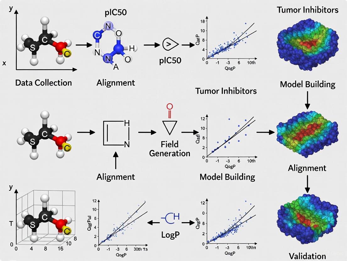
A robust 3D-QSAR workflow involves multiple critical steps from data collection to model application, as illustrated below:

Figure 3: 3D-QSAR Workflow. Key steps include data collection, molecular modeling, alignment, descriptor calculation, model building, validation, interpretation, and compound design.

Data Collection and Preparation: Curate a dataset of compounds with consistently determined biological activities (e.g., IC₅₀, Kᵢ) spanning 3-4 orders of magnitude [20] [1]. Ensure structural diversity while maintaining a common scaffold for meaningful alignment.

Molecular Modeling and Alignment: Generate energetically optimized 3D conformations using molecular mechanics (e.g., UFF) or quantum mechanical methods [1]. Align molecules based on shared pharmacophoric features or maximum common substructure (MCS), assuming similar binding modes [16] [1].

Descriptor Calculation and Model Building: Calculate steric and electrostatic fields (CoMFA) or additional similarity indices (CoMSIA) for aligned molecules [1]. Use Partial Least Squares (PLS) regression to correlate descriptor fields with biological activity, selecting optimal components to avoid overfitting.

Model Validation and Interpretation: Validate models using leave-one-out (LOO) cross-validation (q² > 0.5), external test set prediction (r²ₚᵣₑd > 0.6), and Fischer randomization [20] [16]. Interpret results through 3D contour maps visualizing regions where specific molecular properties enhance or diminish activity.

Applications to Cancer Pathway Inhibition

JAK-STAT Pathway Inhibitors

3D-QSAR has significantly contributed to developing selective JAK inhibitors, particularly for JAK3. A recent study constructed 3D-QSAR models for 73 JAK3 inhibitors with pIC₅₀ values spanning 4 orders of magnitude [16]. The optimal CoMSIA model demonstrated excellent predictive power with q² = 0.52 and r² = 0.91, highlighting key structural features for JAK3 selectivity:

• Hydrophobic moieties at specific positions enhance affinity
• Hydrogen bond acceptors toward certain regions improve selectivity over other JAK isoforms
• Steric bulk in defined areas discriminates against JAK2 binding

The study identified critical residues for selective JAK3 inhibition through molecular dynamics simulations and free energy calculations, facilitating the design of 10 novel inhibitors with predicted high potency [16]. Similarly, field-based 3D-QSAR for JAK-2 inhibitors achieved strong correlation values (r² = 0.884, q² = 0.67), identifying electronegativity, electropositivity, hydrophobicity, and shape as essential determinants of inhibitory activity [21].

Table 2: Selected 3D-QSAR Studies for JAK-STAT Pathway Inhibitors

Target	Method	Statistical Parameters	Key Structural Insights	Reference
JAK3	CoMSIA	q² = 0.52, r² = 0.91	Hydrophobic moieties and H-bond acceptors critical for selectivity	[16]
JAK2	Field-based 3D-QSAR	r² = 0.884, q² = 0.67	Electronegativity, electropositivity, hydrophobicity essential	[21]
SYK	3D-QSAR Pharmacophore	-	One H-bond acceptor, three aromatic rings optimal	[20]

RAS-RAF-MEK-ERK Pathway Inhibitors

The RAS-RAF-MEK-ERK pathway presents multiple targeting opportunities, with 3D-QSAR applications focusing predominantly on RAF and MEK inhibition. Although the search results don't provide detailed 3D-QSAR statistics for this pathway specifically, the successful application of these methods to kinase targets in general suggests strong potential.

Recent efforts have yielded covalent KRASG12C inhibitors like sotorasib (AMG510) and adagrasib (MRTX849), approved for KRASG12C-mutant cancers [17]. While not explicitly detailing 3D-QSAR in their development, these breakthroughs demonstrate the importance of structural optimization approaches that 3D-QSAR facilitates. Resistance mechanisms to these agents highlight the need for continued inhibitor optimization, where 3D-QSAR can contribute significantly.

The pathway's complexity, including feedback regulation and crosstalk with PI3K-AKT-mTOR signaling, presents challenges that 3D-QSAR approaches can address by designing inhibitors with appropriate polypharmacology or combination therapy strategies [17] [19].

Experimental Protocols and Technical Approaches

Detailed 3D-QSAR Protocol for Kinase Inhibitors

Dataset Curation

• Select 20-100 compounds with consistently measured inhibitory activities (IC₅₀) from the same biological assay [20]
• Ensure activity range of 3-4 log units for robust model building
• Divide compounds into training (70-80%) and test sets (20-30%) using structural diversity and activity distribution criteria

Molecular Modeling and Alignment

• Generate 3D structures from 2D representations using tools like RDKit or Sybyl [1]
• Optimize geometries using molecular mechanics (UFF) or semi-empirical methods (AM1)
• Align molecules to a common reference frame using:
  • Maximum Common Substructure (MCS) approach
  • Pharmacophore-based alignment
  • Dock-based alignment using a protein structure if available

Descriptor Calculation and Model Building

• Calculate CoMFA steric and electrostatic fields using sp³ carbon probe with +1 charge
• Compute CoMSIA similarity indices for steric, electrostatic, hydrophobic, and H-bond donor/acceptor fields
• Perform Partial Least Squares (PLS) regression with cross-validation to determine optimal components
• Validate model robustness using leave-one-out (LOO) and leave-many-out cross-validation

Model Application and Compound Design

• Visualize results as 3D contour maps showing favorable/unfavorable regions for steric bulk and electrostatic properties
• Design new analogs incorporating structural features predicted to enhance activity
• Synthesize and test top candidates to validate model predictions

Table 3: Essential Resources for 3D-QSAR Studies in Cancer Pathway Inhibition

Resource Category	Specific Tools/Reagents	Application Purpose	Key Features
Cheminformatics Software	SYBYL, Discovery Studio, RDKit	Molecular modeling, descriptor calculation	Force field implementation, QSAR module integration
3D-QSAR Specialized Tools	CoMFA, CoMSIA modules	Field calculation, contour map generation	Steric/electrostatic field computation, PLS analysis
Molecular Dynamics	AMBER, GROMACS	Binding mode validation, stability assessment	Free energy calculations, trajectory analysis
Protein Data Sources	RCSB PDB	Structural templates for alignment	Experimentally determined protein-ligand complexes
Compound Databases	ZINC, PubChem	Virtual screening, lead identification	Diverse chemical libraries, availability information

3D-QSAR methodologies represent powerful approaches for rational inhibitor design against key cancer pathways like JAK-STAT and RAS-RAF-MEK-ERK. By correlating three-dimensional molecular properties with biological activity, these computational techniques provide valuable insights for optimizing potency, selectivity, and drug-like properties. The integration of 3D-QSAR with complementary approaches like molecular dynamics simulations and free energy calculations enhances predictive accuracy and mechanistic understanding.

Future directions in this field include the incorporation of machine learning algorithms for descriptor selection and model building [22], application to covalent inhibitor design through specialized reaction field descriptors, and addressing compound promiscuity by modeling off-target effects. Additionally, the development of 3D-QSAR models for emerging cancer targets in DNA repair pathways represents a promising avenue for expanding the utility of these methods in oncological drug discovery.

As structural biology and computational power continue to advance, 3D-QSAR approaches will play an increasingly vital role in translating pathway knowledge into effective targeted therapies, ultimately contributing to more personalized and effective cancer treatments.

Field-based Three-Dimensional Quantitative Structure-Activity Relationship (3D-QSAR) modeling has become an indispensable technique in modern computational oncology for designing and optimizing novel tumor inhibitors. Unlike traditional 2D-QSAR methods that use numerical molecular descriptors, 3D-QSAR considers the crucial three-dimensional spatial orientation of molecules, providing insights into how steric (shape-related) and electrostatic fields surrounding a molecule influence its biological activity against cancer targets [1]. This approach is particularly valuable for understanding and overcoming drug resistance mechanisms in cancer therapy, as it allows researchers to visualize specific molecular regions where structural modifications can enhance binding affinity to therapeutic targets [23].

The predictive power and practical utility of 3D-QSAR models fundamentally depend on two critical factors: the quality of specialized software platforms and the rigorous application of validated computational protocols. Software tools enable the accurate calculation of molecular interaction fields, proper alignment of compound datasets, and generation of statistically robust models that can reliably predict the activity of newly designed compounds before costly synthetic efforts [1] [14]. For researchers focusing on tumor inhibitors, mastering these computational tools provides a strategic advantage in accelerating the drug discovery pipeline from initial hit identification to lead optimization stages.

Core 3D-QSAR Methodology and Experimental Protocols

Fundamental Workflow

The construction of a predictive 3D-QSAR model follows a systematic workflow with several interdependent stages. Adherence to this protocol ensures the generation of chemically meaningful and statistically significant models suitable for guiding cancer drug discovery efforts.

Data Collection and Preparation: The process begins with assembling a dataset of compounds with experimentally determined biological activities (e.g., IC₅₀ or Kᵢ values) measured against the cancer target of interest under consistent assay conditions [1]. Activity values are typically converted to negative logarithmic scales (pIC₅₀ = -logIC₅₀) to create a linearly distributed dependent variable for modeling [24]. The dataset should contain structurally related compounds with sufficient diversity to capture meaningful structure-activity relationships, typically divided into training (for model building) and test (for model validation) sets [24] [25].

Molecular Modeling and Conformational Analysis: 2D chemical structures are converted to 3D representations and subjected to geometry optimization using molecular mechanics force fields (e.g., Tripos or MMFF94) or quantum mechanical methods to identify low-energy conformations [1] [24]. For each compound, multiple conformations may be generated and evaluated to identify the putative bioactive conformation, which is often the global energy minimum or a low-energy state compatible with binding [25].

Molecular Alignment: This critical step superimposes all molecules in a common 3D coordinate system that reflects their putative binding orientation at the target site [1]. Alignment methods include:

• Pharmacophore-based alignment: Using common chemical features (hydrogen bond donors/acceptors, hydrophobic centers, aromatic rings) [25]
• Database alignment: Superimposing compounds onto a known active template or reference structure [26]
• Docking-based alignment: Using molecular docking poses to orient compounds within a protein active site [14]
• Maximum Common Substructure (MCS): Identifying and aligning the largest shared structural framework [1]

Descriptor Calculation and Model Building: Following alignment, 3D molecular field descriptors are calculated at grid points surrounding the molecules. In Comparative Molecular Field Analysis (CoMFA), steric (Lennard-Jones) and electrostatic (Coulombic) fields are computed using a probe atom [1]. Comparative Molecular Similarity Indices Analysis (CoMSIA) extends this approach by incorporating additional fields (hydrophobic, hydrogen bond donor/acceptor) using Gaussian-type functions for smoother potential maps [1] [24]. Partial Least Squares (PLS) regression is then used to correlate the field descriptors with biological activity, addressing the high dimensionality and multicollinearity of the descriptor matrix [1] [25].

Model Validation and Interpretation: Rigorous validation assesses model robustness and predictive power. Internal validation uses techniques like Leave-One-Out (LOO) cross-validation, generating cross-validated correlation coefficient (q²) [25]. External validation tests the model on an independent test set not used in training [24]. Statistical metrics include conventional correlation coefficient (r²), standard error of estimate, and F-value [24]. The final model is visualized as 3D contour maps showing regions where specific molecular properties (steric bulk, electropositive/electronegative groups) enhance or diminish biological activity [1].

Workflow Visualization

The following diagram illustrates the comprehensive 3D-QSAR modeling workflow, from initial data preparation to final model application in drug design:

Critical Experimental Parameters and Validation Metrics

Successful 3D-QSAR implementation requires careful attention to technical parameters and validation standards. The table below summarizes key metrics and their acceptable ranges for robust models:

Parameter Category	Specific Metric	Acceptable Range/Value	Technical Significance
Statistical Quality	Regression coefficient (r²)	>0.8 [24] [25]	Measures goodness-of-fit of the model to training data
	Cross-validated r² (q²)	>0.5 [24] [25]	Indicates predictive power through internal validation
	Number of PLS components	Optimized to avoid overfitting [25]	Latent variables capturing variance in descriptor-activity relationship
Data Preparation	Training set size	≥20 compounds [25]	Ensures sufficient statistical power for model development
	Test set size	~20-25% of total dataset [24]	Provides independent validation of model predictability
	Activity range	≥4 orders of magnitude [27]	Ensures adequate dynamic range for meaningful SAR
Field Parameters	Grid spacing	1.0-2.0 Å [25]	Resolution for molecular field calculations
	Probe atom type	sp³ carbon with +1 charge [1]	Standard for steric and electrostatic field calculations

Essential Software Platforms

Specialized software platforms provide the computational infrastructure necessary for implementing the 3D-QSAR workflow described above. The table below summarizes the core capabilities, key features, and typical applications of major commercial and academic platforms relevant to tumor inhibitor research:

Software Platform	Core Capabilities	Key Features for 3D-QSAR	Application in Cancer Research
Forge (Cresset)	Field-based molecular alignment, Activity Atlas, 3D-QSAR model building [25]	FieldTemplater for pharmacophore generation, XED force field, Field-QSAR with PLS regression [25]	Maslinic acid analogs against breast cancer MCF-7 cells (r²=0.92, q²=0.75) [25]
SYBYL (Tripos)	Comprehensive molecular modeling, CoMFA, CoMSIA, molecular docking [24]	CoMFA steric/electrostatic fields, CoMSIA with multiple field types, Region Focusing [24]	Anthraquinone derivatives as PGAM1 inhibitors (CoMFA: q²=0.81, r²=0.97) [24]
Schrödinger	Integrated drug discovery platform, FEP, MM/GBSA, molecular dynamics [28]	Advanced chemical descriptors, QM-Polarized Ligand Docking, Free energy calculations [28]	Predictive modeling for kinase inhibitors and oncology targets [28]
MOE (CCG)	Molecular modeling, simulations, cheminformatics, QSAR, structure-based design [28]	Pharmacophore query development, conformational analysis, descriptor calculation [28]	ADMET prediction, protein engineering for cancer targets [28]
ICM (Molsoft)	Biological system modeling, docking, virtual screening, 3D-QSAR [26]	APF (Atomic Property Fields), flexible superposition to template, PLS regression [26]	Thyroid Hormone Receptor Alpha (THRA) inhibitors [26]

Platform Selection Criteria

Choosing the appropriate software platform depends on several factors specific to the research objectives and available resources:

• Research Stage: For lead optimization with established structure-activity relationships, Forge's field-based approaches offer intuitive visualization. For scaffold hopping and novel chemical matter identification, SYBYL's CoMSIA handles diverse datasets effectively [1] [25].

• Target Information Availability: When protein structure information is available, integrated platforms like Schrödinger that combine 3D-QSAR with docking and molecular dynamics provide enhanced insights. For strictly ligand-based studies, Forge and SYBYL offer specialized functionality [14] [28].

• Computational Resources: Desktop solutions like Forge and SYBYL are suitable for individual researchers, while enterprise platforms like Schrödinger offer scalable solutions for team-based drug discovery programs [28].

• Validation Requirements: Platforms with built-in statistical validation protocols and automated permutation testing ensure model robustness, particularly important for regulatory applications in drug development [24] [25].

Case Studies and Research Applications

Tumor Inhibitor Development Examples

The practical application of 3D-QSAR software in cancer research is illustrated through these representative case studies:

Breast Cancer Inhibitors from Maslinic Acid Analogs: Researchers used Forge software to develop a 3D-QSAR model for maslinic acid analogs tested against MCF-7 breast cancer cells [25]. The study employed FieldTemplater to identify a common pharmacophore from active compounds, followed by field-based alignment of 74 compounds. The resulting model showed excellent statistical parameters (r²=0.92, q²=0.75) and identified key steric and electrostatic features controlling anticancer activity. Virtual screening of a natural product database followed by ADMET filtering identified compound P-902 as a promising candidate, subsequently validated through docking studies against multiple breast cancer targets [25].

PGAM1 Inhibitors for Cancer Metabolism Therapy: In a study targeting phosphoglycerate mutase 1 (PGAM1), a key enzyme in cancer metabolism, researchers utilized SYBYL to perform both CoMFA and CoMSIA analyses on anthraquinone derivatives [24]. The models demonstrated high predictive power (CoMFA: q²=0.81, r²=0.97; CoMSIA: q²=0.82, r²=0.96) and contour maps revealed structural requirements for PGAM1 inhibition. Molecular dynamics simulations validated the binding modes of newly designed compounds, with specific residues (F22, K100, V112, W115, R116) identified as critical for inhibitor binding [24].

NAMPT Inhibitors for Cancer Therapy: A field-based 3D-QSAR study on amide- and urea-containing NAMPT inhibitors employed docking-based alignment to generate predictive models [14]. The optimized model successfully identified key molecular interactions with active site residues, enabling rational design of novel inhibitors with potential applications against various cancers dependent on the NAD+ salvage pathway [14].

Integrated Computational Approaches

Modern 3D-QSAR studies increasingly combine multiple computational techniques to enhance predictive accuracy and mechanistic understanding:

3D-QSAR with Molecular Dynamics: Integration of 3D-QSAR with molecular dynamics (MD) simulations allows for incorporation of protein flexibility and explicit solvent effects. In the SYK kinase inhibitor study, 3D-QSAR pharmacophore models were used for virtual screening, with MD simulations providing validation of binding stability and key protein-ligand interactions [27].

3D-QSAR with Free Energy Calculations: Advanced platforms like Schrödinger incorporate free energy perturbation (FEP) calculations to refine 3D-QSAR predictions with rigorous thermodynamic binding estimates [28].

The following diagram illustrates how these computational techniques integrate into a comprehensive drug discovery workflow for tumor inhibitor development:

Research Reagent Solutions

Successful implementation of 3D-QSAR studies requires both computational tools and conceptual "research reagents" - the fundamental components and data resources that form the foundation of reliable models.

Research Reagent	Function in 3D-QSAR	Implementation Examples
Curated Bioactivity Data	Provides experimental activity values for model training and validation	IC₅₀ values from uniform bioassays [24] [25]; pKd values from binding assays [26]
Molecular Force Fields	Calculates molecular energies and optimizes 3D geometries	Tripos force field [24]; XED force field [25]; Universal Force Field (UFF) [1]
Structural Templates	Provides reference frameworks for molecular alignment	Known active compounds [25]; Protein Data Bank structures [26]; Pharmacophore hypotheses [27]
Chemical Descriptors	Numerically represents molecular properties for QSAR	Steric and electrostatic field points [1] [25]; Similarity indices [1]; Quantum chemical parameters [28]
Validation Protocols	Assesses model robustness and predictive power	Leave-One-Out cross-validation [25]; Test set prediction [24]; Fisher randomization [27]

Field-based 3D-QSAR methodologies, implemented through sophisticated software platforms like Forge, SYBYL, and their counterparts, provide powerful capabilities for rational design of tumor inhibitors. The integration of these computational approaches with experimental validation creates an iterative cycle of compound optimization that significantly accelerates oncology drug discovery. As these platforms continue to evolve with enhanced AI capabilities, improved force fields, and more intuitive interfaces, their impact on overcoming cancer drug resistance and identifying novel therapeutic strategies will undoubtedly expand. For research teams engaged in tumor inhibitor development, strategic investment in both the computational tools and expertise required for 3D-QSAR modeling represents a valuable approach to addressing the persistent challenge of cancer drug discovery.

The discovery and optimization of tumor inhibitors represent a critical frontier in the battle against cancer. Among the modern computational techniques employed, field-based Three-Dimensional Quantitative Structure-Activity Relationship (3D-QSAR) modeling has emerged as a powerful tool for rational drug design. This methodology correlates the three-dimensional structural and field properties of compounds with their biological activity against specific oncology targets, enabling the prediction and design of more potent inhibitors. The reliability of any 3D-QSAR model is fundamentally contingent on the quality, consistency, and appropriate preparation of the underlying data. This guide details the core data requirements—encompassing compound selection, activity data curation, and structural preparation—essential for initiating robust 3D-QSAR studies focused on tumor inhibitors.

Compound Selection and Dataset Curation

The initial and perhaps most crucial step in a 3D-QSAR study is the assembly of a high-quality dataset of inhibitory compounds.

Sourcing and Selection Criteria

Information on kinase inhibitor activity can be retrieved from public chemical and bioactivity databases such as ChEMBL, BindingDB, and Excape [29]. When selecting compounds from these sources, researchers should apply stringent criteria. For instance, in a study on RET kinase inhibitors, the selection was refined to data from wild-type, non-cell-based assays where the inhibitory concentration (IC50) was measured in nanomolar (nM) units [29]. This ensures data homogeneity. Furthermore, compounds with activity annotations featuring blank fields or values containing “<” or “>” should typically be excluded to maintain data integrity [29].

The selected compounds should be structurally related to ensure coherent modeling, yet sufficiently diverse to capture meaningful structure-activity relationships [1]. A common strategy involves focusing on a specific chemotype or core structure that interacts with a key region of the target protein. For example, many selective RET inhibitors share a 5,6-fused bicyclic ring that acts as a hinge binder, making this a suitable scaffold for building a focused dataset [29].

Dataset Division for Modeling and Validation

Once a curated dataset is assembled, it must be divided into a training set and a test set. The training set is used to build the QSAR model, while the test set is reserved for an external validation of its predictive power. A common practice is to use a 3:1 or 9:1 ratio for the training and test sets, respectively [29] [30]. The division should be performed via random selection, sometimes with the additional step of grouping compounds into high, medium, and low activity bands first to ensure the test set is representative of the entire activity range [30].

Table 1: Public Databases for Sourcing Tumor Inhibitor Data

Database Name	Primary Content	Utility in 3D-QSAR
ChEMBL [29]	Bioactive molecules with drug-like properties, curated from scientific literature.	A primary source for consistent bioactivity data (e.g., IC50) for a wide range of oncology targets.
BindingDB [29]	Binding affinities for protein-ligand complexes.	Provides binding data useful for modeling receptor-ligand interactions.
Excape [29]	Database of chemical structures and associated biological activities.	Another source for retrieving compound and activity data for dataset building.
Protein Data Bank (PDB) [5]	3D structural data for biological macromolecules.	Source of crystal structures for molecular docking and receptor-guided alignment.

Diagram 1: Compound selection and curation workflow.

Activity Data: Measurement and Transformation

Biological activity data is the dependent variable in any QSAR model and must be handled with care to ensure statistical soundness.

Activity Measurements and Conversion

The most common measurement for inhibitory activity is the half-maximal inhibitory concentration (IC50), typically reported in molar units (e.g., nM, µM) [29] [6]. To minimize skewness and linearize the relationship between the concentration and the modeled response, IC50 values are converted into their negative logarithmic form, pIC50, using the following formula [29] [6]: pIC50 = –log10(IC50) In practice, to handle unit conversion seamlessly, the formula is often expressed as: pIC50 = 9 – log(IC50) for IC50 values in nM [29], or pIC50 = –log10(IC50 × 10⁻⁶) for IC50 values in µM [6]. This transformation results in a positive value where a higher pIC50 indicates greater potency.

Data Uniformity and Integrity

All activity data for the training set must be acquired under uniform experimental conditions [1]. Variability in assay protocols (e.g., cell-based vs. non-cell-based, different cell lines) introduces unwanted noise and systemic bias, which can severely compromise the predictive value and interpretability of the final QSAR model.

Table 2: Biological Activity Data Handling in 3D-QSAR

Data Aspect	Description	Best Practice
Activity Type	Direct measure of compound potency (e.g., IC50, Ki).	Use IC50 values from consistent, biochemical, non-cell-based assays for initial model development [29].
Value Transformation	Converting IC50 to pIC50 for modeling.	Apply the formula pIC50 = -log10(IC50) to create a linear, normally-distributed response variable [29] [6].
Data Integrity	Handling of incomplete or uncertain data.	Exclude compounds with activity annotations containing ">", "<", or blank fields to ensure a reliable dataset [29].
Experimental Consistency	Ensuring data is generated from comparable assays.	Collect all activity data from the same type of assay (e.g., wild-type, non-cell-based) under standardized conditions [29] [1].

Structural Preparation and Molecular Modeling

The accurate generation and preparation of 3D molecular structures form the foundation for all subsequent alignment and descriptor calculation steps.

Generation of 3D Structures and Conformer Sampling

The process typically begins with two-dimensional (2D) structural sketches, which are created using software like PerkinElmer ChemDraw [6]. These 2D structures are then converted into three-dimensional coordinates using molecular modeling packages such as Spartan or Schrödinger's LigPrep [6] [29]. This 2D-to-3D conversion may include options for neutralizing compounds and generating possible states or tautomers [29].

The resulting initial 3D structures are not necessarily in their lowest energy or bioactive conformation. Therefore, they must undergo geometry optimization. This can be achieved using molecular mechanics force fields (e.g., Tripos force field, OPLS3e, or the Universal Force Field (UFF)) or, for higher accuracy, quantum mechanical methods like Density Functional Theory (DFT) with a basis set such as B3LYP/6-31G* [6] [29] [1]. Since molecules are flexible, generating multiple low-energy conformers for each compound is often necessary to account for flexibility and aid in identifying the putative bioactive conformation [1].

Molecular Docking for Receptor-Guided Alignment

A powerful approach for structural preparation, especially when a protein crystal structure is available, is molecular docking. It is used to pose compounds into the target's binding site, providing a receptor-guided alignment for 3D-QSAR [29]. The general protocol involves:

• Protein Preparation: A crystal structure of the target (e.g., from the Protein Data Bank) is prepared by adding hydrogen atoms, removing unnecessary chains and water molecules, and correcting any faulty amino acid residues. The protein structure is then minimized using a force field like OPLS3e to an acceptable RMSD (e.g., 0.3 Å) [29].
• Grid Generation: A grid box is defined around the centroid of the native ligand or the known binding site.
• Ligand Docking: The prepared ligands are docked into the binding site using software like Glide [29]. The docking pose that forms key interactions with hinge region residues (e.g., hydrogen bonds with ALA807 or GLU805 in RET kinase) is often selected for QSAR modeling [29]. The docking model itself must be validated by redocking the native crystal ligand and calculating the RMSD between the redocked and original poses [29].

Diagram 2: Structural preparation and alignment workflow.

The Scientist's Toolkit: Essential Research Reagents and Software

Table 3: Essential Computational Tools for 3D-QSAR of Tumor Inhibitors

Tool / Reagent	Category	Function in 3D-QSAR Workflow
KNIME [29]	Data Analytics Platform	Used for data curation, compilation, and preprocessing of compounds and activity data from various sources.
Schrödinger Suite (LigPrep, Glide, Maestro) [29] [31]	Molecular Modeling Software	Provides an integrated environment for ligand preparation (LigPrep), molecular docking (Glide), and field-based QSAR model building and visualization.
Sybyl/SYBYL-X [6] [5]	Molecular Modeling Software	A classic software package for conducting CoMFA and CoMSIA studies, including molecular alignment and PLS analysis.
RDKit [1]	Cheminformatics Library	An open-source toolkit for cheminformatics, useful for 2D-to-3D conversion, molecular alignment, and descriptor calculation.
Protein Data Bank (PDB) [5]	Structural Database	The single worldwide repository for 3D structural data of proteins and nucleic acids, essential for obtaining target structures for docking.
ChEMBL / BindingDB [29]	Bioactivity Database	Public databases used to retrieve experimental bioactivity data (e.g., IC50) for compounds against specific oncology targets.
Tripos Force Field [5]	Molecular Mechanics Force Field	Used for energy minimization and geometry optimization of molecular structures.
Gasteiger-Hückel Charges [5]	Partial Charge Calculation	A method for assigning partial atomic charges to molecules, which are critical for calculating electrostatic fields and docking simulations.
Partial Least Squares (PLS) [29] [6]	Statistical Method	The core regression technique used to build the relationship between 3D molecular field descriptors and biological activity.

A meticulous approach to data collection and preparation is the bedrock of a successful and predictive 3D-QSAR model for tumor inhibitors. This involves the careful selection and curation of compounds from reliable databases, the rigorous transformation and standardization of biological activity data, and the precise generation and optimization of 3D molecular structures, often guided by molecular docking. Adherence to these detailed protocols for compound selection, activity data handling, and structural preparation, as outlined in this guide, will equip researchers with a robust foundation for embarking on field-based 3D-QSAR studies, ultimately accelerating the discovery of novel and potent anti-cancer therapeutics.

Building Your 3D-QSAR Model: A Step-by-Step Workflow for Tumor Inhibitors

Quantitative Structure-Activity Relationship (QSAR) modeling represents a cornerstone of modern computational drug discovery, providing a predictive framework that correlates the chemical structure of compounds with their biological activity. When extended to three dimensions, 3D-QSAR offers superior capability in rational drug design by incorporating spatial and electronic properties that dictate molecular recognition and binding. In the context of tumor inhibitor research, field-based 3D-QSAR techniques implemented in platforms like Forge and SYBYL enable researchers to quantitatively understand how structural features influence anticancer activity, guiding the optimization of lead compounds with improved potency and selectivity.

The fundamental principle underlying 3D-QSAR is that biological activity can be correlated with interaction fields surrounding molecules, typically steric (shape-related) and electrostatic (charge-related) fields. Unlike traditional 2D-QSAR that uses molecular descriptors invariant to conformation, 3D-QSAR derives descriptors directly from the spatial structure of molecules, providing finer resolution of molecular interactions but introducing challenges related to molecular alignment and conformational sampling. For oncology targets, this approach has been successfully applied to various kinase inhibitors, including those targeting RET, BRAF, Plk1, and other key players in cancer signaling pathways.

Theoretical Foundations and Biological Context

Key Signaling Pathways in Cancer

Cancer pathogenesis frequently involves dysregulation of essential signaling pathways that control cell growth, proliferation, and survival. Understanding these pathways provides biological context for 3D-QSAR studies on tumor inhibitors. The following diagram illustrates a prominent pathway frequently targeted in cancer drug discovery:

This pathway is particularly significant in melanoma, where the BRAFV600E mutation occurs in 70-90% of cases, making it a prime target for inhibitor development. BRAF inhibitors like dabrafenib and vemurafenib exemplify successful targeting of this pathway, with their discovery and optimization benefiting from computational approaches including 3D-QSAR.

3D-QSAR methods like Comparative Molecular Field Analysis (CoMFA) and Comparative Molecular Similarity Indices Analysis (CoMSIA) operate on the principle that biological activity can be correlated with interaction fields surrounding molecules. The key distinction between traditional QSAR and 3D-QSAR lies in their descriptor systems:

• Classical QSAR: Uses summary descriptors (e.g., logP, molar refractivity) that are invariant to molecular conformation and orientation.
• 3D-QSAR: Derives descriptors from spatial structure and interaction fields calculated at grid points surrounding aligned molecules, making them conformation-dependent.

The table below compares the main 3D-QSAR approaches:

Table 1: Comparison of Primary 3D-QSAR Methodologies

Method	Field Types	Alignment Sensitivity	Key Advantages	Common Applications
CoMFA	Steric, Electrostatic	High	Established method, easily interpretable contour maps	Congeneric series with reliable alignment
CoMSIA	Steric, Electrostatic, Hydrophobic, H-bond Donor/Acceptor	Moderate	Smoother fields, additional field types, more tolerant to alignment variations	Structurally diverse datasets
Field-Based 3D-QSAR in Forge	Steric, Electrostatic, Hydrophobic, etc.	Configurable	Advanced statistics, robust validation, intuitive visualization	Lead optimization throughout drug discovery pipeline

Experimental Setup and Workflow Design

Data Collection and Curation

The foundation of any robust QSAR model is a high-quality, curated dataset of compounds with reliable biological activity data. For tumor inhibitor research, this typically involves collecting IC₅₀ or Kᵢ values from published literature or experimental work.

Data Collection Protocols:

• Source Identification: Extract compound structures and activity data from public databases (ChEMBL, BindingDB) or proprietary corporate databases. For RET kinase inhibitors, one study compiled 952 inhibitors with 49 different 5,6-fused bicyclic heteroaromatic rings from five data sources [29].
• Activity Standardization: Convert all activity measurements to a consistent format (typically pIC₅₀ = -logIC₅₀) and unit (nM). Exclude compounds with ambiguous activity annotations (e.g., containing "<" or ">") [29].
• Structural Curation: Remove duplicates, standardize tautomeric states, and address salt forms. Utilize automated workflows in KNIME or other platforms for efficient data preprocessing [32].
• Chemical Space Analysis: Apply statistical molecular design (SMD) and principal component analysis (PCA) to evaluate structural diversity and ensure adequate coverage of chemical space [33].

Key Considerations for Tumor Inhibitors:

• Focus on compounds tested against specific oncology targets (e.g., BRAFV600E, RET, Plk1)
• Ensure consistent assay conditions (e.g., non-cell-based vs. cell-based)
• Document mutation status of molecular targets when relevant

Molecular Modeling and Conformation Generation

Accurate 3D molecular structures are prerequisite for field-based QSAR analyses. Multiple approaches exist for generating biologically relevant conformations:

Methodology:

• 2D to 3D Conversion: Transform 2D structures to 3D coordinates using tools like RDKit, LigPrep (Schrödinger), or CORINA.
• Geometry Optimization: Minimize structures using molecular mechanics force fields (e.g., OPLS3e, MMFF94) or quantum mechanical methods for higher accuracy [29] [1].
• Conformational Sampling: Generate multiple low-energy conformations for each compound using systematic search, stochastic methods, or rule-based approaches. For pyrazole-based TRAP1 inhibitors, conformational ensembles were generated to account for flexibility [34].

Software-Specific Implementation in Forge:

• Utilize the built-in conformation generator with options for energy window and maximum conformers
• Consider the "global minimum" or "diverse" conformation generation strategies based on dataset size
• For large datasets, balance computational cost with conformational coverage (typically 10-50 conformers per compound)

Molecular Alignment Strategies

Molecular alignment constitutes the most critical step in 3D-QSAR, as field descriptors are sensitive to relative molecular orientation. The alignment should reflect putative bioactive conformations:

Common Alignment Protocols:

Table 2: Molecular Alignment Methods for 3D-QSAR

Method	Procedure	Applicability	Limitations
Pharmacophore-Based	Align compounds based on common chemical features (H-bond donors/acceptors, hydrophobic regions)	Diverse chemotypes with shared pharmacophore	Requires reliable pharmacophore hypothesis
Maximum Common Substructure (MCS)	Identify largest common substructure and use for alignment	Structurally related series with variable substituents	May fail for highly diverse compounds
Docking-Based	Use molecular docking poses against target protein structure	When crystal structure available and binding mode consistent	Computationally intensive, dependent on docking accuracy
Scaffold-Based	Align using core scaffold (e.g., Bemis-Murcko scaffolds)	Series with well-defined common core	Neglects conformational flexibility of side chains

Case Example - RET Kinase Inhibitors: For 5,6-fused bicyclic heteroaromatic derivatives targeting RET kinase, researchers performed receptor-guided alignment using molecular docking simulations. The crystal structure of RET complex (PDB ID: 7DUA) was prepared, and compounds were docked with constraints to form hydrogen bonds with hinge residues ALA807 or GLU805 [29]. This approach ensured consistent orientation in the biologically relevant binding mode.

Descriptor Calculation and Field Generation

With aligned molecules, the next step involves calculating interaction fields that serve as molecular descriptors:

Standard Protocol:

• Grid Definition: Create a 3D grid that encompasses all aligned molecules with typical spacing of 1.0-2.0 Å.
• Probe Selection: Choose appropriate probe atoms (typically sp³ carbon with +1 charge for CoMFA).
• Field Calculation:
  • Steric Fields: Lennard-Jones potential measured at each grid point
  • Electrostatic Fields: Coulomb potential calculated at each grid point
  • Hydrophobic Fields: In CoMSIA, additional hydrophobic and hydrogen-bonding fields

Forge-Specific Implementation:

• Select field types based on target biology (e.g., emphasize hydrophobic fields for targets with extensive hydrophobic pockets)
• Adjust grid padding to ensure complete molecular coverage (typically 4-6 Å beyond molecular extents)
• Consider smoothing functions (Gaussian in CoMSIA) to reduce abrupt field changes

Model Building and Validation Framework

Statistical Modeling using Partial Least Squares (PLS)

Field-based 3D-QSAR typically employs Partial Least Squares regression due to its ability to handle large, collinear descriptor matrices:

Model Building Protocol:

• Data Splitting: Divide dataset into training (≈80%) and test (≈20%) sets using random, stratified, or structure-based splitting.
• PLS Factor Determination: Use cross-validation to determine optimal number of latent variables that maximizes predictivity without overfitting.
• Model Generation: Build regression model correlating field values with biological activity.

Case Example - Statistical Parameters: In a 3D-QSAR study of RET kinase inhibitors, the optimal model exhibited R² (training) = 0.801 and Q² (test) = 0.794, indicating high predictive performance [29]. For pyrimidine-sulfonamide hybrids as BRAFV600E inhibitors, similar statistical rigor was applied [35].

Model Validation Strategies

Robust validation is essential to ensure model reliability and predictive power:

Validation Protocols:

• Internal Validation:
  • Leave-One-Out (LOO) cross-validation
  • Leave-Many-Out (LMO) cross-validation with multiple groups
• External Validation: Predict activity of completely excluded test set compounds
• Additional Validation:
  • Y-scrambling to exclude chance correlations
  • Applicability domain analysis to define chemical space where predictions are reliable

Advanced Validation Example: For the RET kinase inhibitor model, researchers performed double verification using patent-filed RET inhibitors as an out-of-set third dataset that never included either training or test data, demonstrating acceptable residual analysis results [29].

Model Interpretation and Visualization

The primary advantage of 3D-QSAR lies in the intuitive visualization of structure-activity relationships:

Interpretation Methodology:

• Contour Map Generation: Create 3D isosurfaces indicating regions where specific molecular features enhance or diminish activity.
• Structure-Activity Analysis: Correlate contour regions with specific structural features in active and inactive compounds.
• Design Hypothesis Formulation: Develop rationale for molecular modifications to improve activity.

Visualization Guidelines:

• Green contours: Regions where steric bulk increases activity
• Yellow contours: Regions where steric bulk decreases activity
• Blue contours: Regions where positive charge increases activity
• Red contours: Regions where negative charge increases activity

Integrated Workflow for Tumor Inhibitor Research

The complete 3D-QSAR workflow for tumor inhibitor research integrates multiple computational components into a coherent pipeline as illustrated below:

Essential Research Reagent Solutions

Successful implementation of 3D-QSAR for tumor inhibitor research requires both computational tools and experimental components:

Table 3: Essential Research Reagents and Computational Tools for 3D-QSAR

Category	Specific Tools/Reagents	Function	Application Example
Computational Platforms	Forge V12 (Cresset), SYBYL-X (Certara)	Primary environment for 3D-QSAR model development	Field alignment, PLS analysis, contour visualization
Docking Software	Glide (Schrödinger), GOLD (CCDC)	Receptor-guided alignment and binding mode analysis	Docking poses for alignment of RET inhibitors [29]
Protein Structures	PDB IDs: 7DUA (RET), 5Y3N (TRAP1), 4BJX (BRD4)	Structural templates for docking-guided alignment	Understanding binding interactions for rational design
Compound Databases	ChEMBL, BindingDB, ZINC, Enamine	Sources of structural and activity data for model building	Retrieving BRAF and RET inhibitor datasets [29] [35]
Workflow Automation	KNIME, PipelinePilot	Automated data curation and modeling pipelines	Streamlining QSAR model building process [32]
Chemical Features	Hydrogen bond donors/acceptors, hydrophobic groups, aromatic rings	Defining pharmacophore hypotheses for alignment	DHHRR pharmacophore for TRAP1 inhibitors [34]

Establishing a robust 3D-QSAR workflow in Forge/SYBYL for tumor inhibitor research requires meticulous attention to each step of the process, from data curation through model validation. By implementing the protocols and methodologies outlined in this guide, researchers can develop predictive models that effectively guide the optimization of anticancer agents. The integration of computational predictions with experimental validation creates an iterative cycle of compound design and optimization, accelerating the discovery of novel tumor inhibitors with improved potency and selectivity profiles.

As the field advances, the increasing availability of high-quality structural and activity data, combined with more sophisticated algorithms for conformational sampling and alignment, will further enhance the predictive power of 3D-QSAR approaches in oncology drug discovery. The workflow described here provides a solid foundation that can be adapted to specific research needs and extended as new methodologies emerge.

In the realm of rational drug design, particularly for tumor inhibitors, three-dimensional Quantitative Structure-Activity Relationship (3D-QSAR) models serve as powerful predictive tools for designing novel compounds with enhanced potency and selectivity. The fundamental principle of 3D-QSAR is that deviations in biological response among a series of compounds are accountable for the differences in their spatial and structural properties, moving beyond simple molecular descriptors to consider the full three-dimensional characteristics of molecules [3]. Unlike classical 2D-QSAR methods, 3D-QSAR exploits the 3D properties of ligands—such as steric bulk, electrostatic potential, and hydrophobic interactions—to predict biological response using robust chemometric tools [3]. The accuracy and predictive power of these models, including widely used methods like Comparative Molecular Field Analysis (CoMFA) and Comparative Molecular Similarity Indices Analysis (CoMSIA), are critically dependent on two foundational steps: the judicious selection of reference compounds and the accurate determination of their bioactive conformations [1] [3]. These initial steps establish the spatial framework upon which all subsequent molecular alignments and field calculations are built, ultimately determining the success or failure of the entire 3D-QSAR endeavor in tumor inhibitor research.

Selecting Reference Compounds for Tumor Inhibitor Research

The selection of reference compounds forms the cornerstone of a reliable 3D-QSAR model. These compounds serve as the structural templates for molecular alignment and define the chemical space explored by the model.

Key Criteria for Reference Compound Selection

• Structural Diversity and Relationship: The dataset should comprise compounds that are structurally related to ensure coherent modeling, yet sufficiently diverse to capture meaningful structure-activity relationships (SAR). This balance allows the model to identify critical structural features responsible for biological activity against tumor targets [1].
• Uniform and Precise Biological Data: All compounds must have biological activity data (e.g., IC₅₀, GI₅₀) determined under uniform experimental conditions against the specific tumor-related target, such as Bcr-Abl for chronic myeloid leukemia [13] [3]. The integrity of this dataset is paramount, as variability in assay protocols introduces noise and systemic bias, compromising the model's predictive value [1].
• Potency Range: The dataset should encompass a broad range of biological activities, from highly active to moderately or weakly active compounds. This range is essential for the model to discern the structural features that enhance or diminish potency [36].
• Presence of a Common Scaffold: Ideally, compounds should share a common molecular scaffold or core structure, such as the purine scaffold in Bcr-Abl inhibitors [13] or the imidazo-pyridine derivatives in dual AT1 antagonists and PPARγ partial agonists [37]. This common core facilitates more reliable molecular alignment.

Exemplary Reference Compound Set for Bcr-Abl Inhibition

The following table summarizes a representative dataset of purine-based Bcr-Abl inhibitors, which could serve as a reference for building a 3D-QSAR model targeting chronic myeloid leukemia [13].

Table 1: Exemplary Reference Compounds for Bcr-Abl Tumor Inhibition

Compound ID	Core Scaffold	Key Substituents	Bcr-Abl IC₅₀ (μM)	Cell-Based GI₅₀ (μM)	Key Feature
Imatinib	Not Applicable	(Reference Drug)	0.33	Varies by cell line	First-line TKI
7a	Purine	Specific 2,6,9-modifications	0.13	Data from source [13]	Higher potency than Imatinib
7c	Purine	Specific 2,6,9-modifications	0.19	0.30 (K562 cells)	High potency, lower toxicity
7e / 7f	Purine	Specific 2,6,9-modifications	Data from source [13]	13.80 / 15.43 (KCL22-B8)	Active against T315I mutant
Compound VII	Purine	Cyclopropylmethyl at N-9	0.015	0.7-1.3 (CML lines)	High potency, active against mutants

Determining Bioactive Conformations

The bioactive conformation is the specific three-dimensional arrangement of a molecule's atoms when it is bound to its biological target. Accurately determining this conformation is arguably the most critical and challenging step in 3D-QSAR model development [3].

Experimental Methods for Bioactive Conformation Determination

• X-ray Crystallography: This method provides the precise 3D structure of macromolecule-ligand complexes. Drug-receptor complexes obtained by X-ray crystallography offer the most definitive information on bioactive conformations [3].
• Nuclear Magnetic Resonance (NMR) Spectroscopy: NMR can be used to study the conformations of ligands bound to receptors, providing information in a solution state that may be more physiologically relevant than crystal structures [3].

Computational Methods for Bioactive Conformation Determination

When experimental data is unavailable, computational techniques are employed to propose likely bioactive conformations.

• Molecular Docking: Docking simulations predict the preferred orientation of a molecule within a protein's binding pocket. As demonstrated in studies of Bcr-Abl [13] and dual AT1/PPARγ inhibitors [37], docking can elucidate key interactions (e.g., hydrogen bonds with Tyr35, Arg167, and Lys199 in AT1) and validate the binding mode of a proposed bioactive conformation.
• Conformational Analysis and Search: This involves systematically exploring the low-energy conformations of a molecule using methods such as:
  • Systematic Search: Rotating torsion angles through a full range of values.
  • Monte Carlo Methods: Using random changes to generate diverse conformers.
  • Molecular Dynamics Simulations: Simulating the physical movements of atoms over time to explore the conformational space [3].

The workflow for determining the bioactive conformation is a multi-step process, as illustrated below:

Diagram 1: Workflow for determining the bioactive conformation of a reference compound.

Integrated Workflow and Practical Protocol

Integrating the selection of reference compounds and the determination of their bioactive conformations leads to a robust, practical protocol for initiating a 3D-QSAR study on tumor inhibitors.

Integrated Experimental Protocol

Phase 1: Data Curation and Preparation

• Define the Structural and Activity Scope: Compile a dataset of 20-50 compounds with a common scaffold (e.g., purine for kinase inhibitors [13]) and a consistent, quantitative biological activity measure (e.g., IC₅₀) against a specific tumor target [1] [3].
• Generate Initial 3D Structures: Convert 2D molecular representations into 3D coordinates using cheminformatics tools like RDKit or Sybyl [1].
• Geometry Optimization: Refine the initial 3D structures by minimizing their conformational energies using molecular mechanics (e.g., UFF) or higher-accuracy quantum mechanical methods to achieve realistic, low-energy conformations [1] [3].

Phase 2: Bioactive Conformation Analysis

• Identify a Template: Select the most potent and rigid compound from the dataset as the initial template for alignment.
• Determine Bioactive Conformations: For each compound, apply the workflow in Diagram 1. Prioritize using conformations from experimental co-crystal structures. If unavailable, use molecular docking and dynamics simulations to propose the most likely bioactive conformation, as demonstrated in studies of Bcr-AblT315I [13] and PPARγ agonists [37].
• Molecular Alignment: Superimpose all molecules in the dataset onto the template's bioactive conformation. This can be achieved by aligning based on a maximum common substructure (MCS) or using field-based alignment methods like the AlphaQ protocol, which optimizes quantum mechanical cross-correlation for structurally diverse sets [36]. The alignment assumes all compounds share a similar binding mode to the target [1].

The following diagram illustrates this integrated, iterative process from compound selection to model-ready alignment.

Diagram 2: The critical path from reference compound selection to a aligned dataset for 3D-QSAR.

Table 2: Essential Research Reagents and Computational Tools for 3D-QSAR

Category	Item / Software	Function / Application
Computational Tools	Sybyl (Tripos)	Industry-standard suite for CoMFA/CoMSIA studies, molecular modeling, and alignment [1].
	RDKit	Open-source cheminformatics toolkit for generating 3D structures, MCS-based alignment, and descriptor calculation [1].
	AutoDock Vina, GOLD	Molecular docking software to predict binding modes and propose bioactive conformations [13] [37].
	GROMACS, AMBER	Software for molecular dynamics simulations to refine conformations and study protein-ligand stability [13].
Data & Database	ChEMBL	Public database of bioactive molecules with drug-like properties to source activity data and compounds [38].
	Protein Data Bank (PDB)	Repository for 3D structural data of proteins and protein-ligand complexes to obtain bioactive templates [3].
	Cambridge Structural Database (CSD)	Repository for small-molecule organic and metal-organic crystal structures [3].
Methodology	CoMFA/CoMSIA	Core 3D-QSAR methods to correlate steric/electrostatic fields with biological activity [13] [1] [3].
	PLS Regression	Statistical method to build the predictive model linking 3D descriptors to activity [1] [3].

The rigorous selection of reference compounds and the accurate determination of their bioactive conformations are not merely preliminary steps but the very foundation upon which predictive and chemically intuitive 3D-QSAR models are built. In the context of tumor inhibitor research, where the strategic design of molecules to overcome drug resistance is paramount—as seen with Bcr-AblT315I mutations [13]—these initial decisions dictate the model's ability to guide synthetic efforts toward more potent and selective therapeutics. By adhering to the principles and protocols outlined in this guide, researchers can establish a solid groundwork for developing 3D-QSAR models that truly illuminate the structure-activity landscape and accelerate the discovery of next-generation oncology agents.

The reliability of any three-dimensional Quantitative Structure-Activity Relationship (3D-QSAR) model is fundamentally dependent on the initial steps of dataset preparation. For research focused on tumor inhibitors, rigorous dataset curation ensures that predictive models accurately capture the structural features governing biological activity. This process involves the careful selection of compounds with experimentally determined activities (such as IC₅₀ values), the strategic division of the dataset into training and test sets, and the critical step of molecular alignment. Molecular alignment superimposes all molecules within a shared 3D reference frame, which is a prerequisite for calculating the spatial molecular descriptors (like steric and electrostatic fields) that form the basis of field-based 3D-QSAR methods such as Comparative Molecular Field Analysis (CoMFA) and Comparative Molecular Similarity Indices Analysis (CoMSIA) [1]. The following sections provide a detailed technical guide to these foundational protocols, framed within the context of developing tumor inhibitor models.

Training-Test Set Division Methodologies

A critical step in QSAR model development is the division of the full dataset into training and test sets. The training set is used to build the model, while the independent test set is reserved exclusively for the final assessment of the model's predictive performance on unseen data [39]. A proper split is essential to avoid overfitting and to generate a model with robust generalizability.

Data Collection and Cleaning

Before any division, the dataset must be curated:

• Compile Data: Assemble chemical structures and associated biological activities from reliable literature or databases. For tumor inhibitor research, this typically involves compounds with cytotoxic activities (e.g., pIC₅₀ = -logIC₅₀) against specific cancer cell lines [40].
• Standardize Structures: Remove salts, normalize tautomers, and handle stereochemistry consistently [39].
• Ensure Uniform Activity Data: All biological activities should be determined under uniform experimental conditions and converted to a common scale (e.g., log-transform) to minimize noise [1].

Division Strategies and Protocols

The choice of how to split the data can significantly impact the model's perceived performance. Two common methods are random selection and algorithms designed to ensure representativeness.

Detailed Protocol: Random Division

• Procedure: After standardizing the dataset, assign a random number to each compound. A common practice is to use about 80% of the compounds for training and the remaining 20% for the external test set [40].
• Validation: After the split, check that the test set covers a similar chemical space and activity range as the training set to ensure it is representative.

Detailed Protocol: Kennard-Stone Algorithm

• Objective: This algorithm selects a test set that is uniformly distributed over the chemical space defined by the molecular descriptors, ensuring the training set spans the entire range of structural features [39].
• Procedure: The algorithm works by iteratively selecting the compound that is farthest from those already in the training set until the desired number of test compounds is reached.

Table 1: Comparison of Training-Test Set Division Methods

Method	Key Principle	Advantages	Limitations	Suitability for Tumor Inhibitor Studies
Random Division [40]	Arbitrary random selection of compounds.	Simple and fast to implement.	Risk of creating non-representative sets if the dataset is small or clustered.	Suitable for large, diverse datasets of tumor inhibitors.
Kennard-Stone Algorithm [39]	Selects samples to uniformly cover the descriptor space.	Ensures the training set is representative of the entire chemical space; improves model reliability.	More computationally intensive than random selection.	Highly recommended for ensuring model robustness across diverse chemotypes of inhibitors.

Molecular Alignment Strategies

Molecular alignment is one of the most critical and demanding steps in 3D-QSAR. The objective is to superimpose all molecules in a shared 3D coordinate system based on a presumed common binding mode to the biological target [1]. A poor alignment introduces noise and can severely undermine the model's predictive ability and interpretability.

Pre-alignment Molecular Modeling

Before alignment, 2D molecular structures must be converted into realistic 3D conformations.

• 3D Structure Generation: Use cheminformatics tools like RDKit or Sybyl to convert 2D representations (e.g., SMILES strings) into 3D coordinates [1].
• Geometry Optimization: The initial 3D structures are then energy-minimized using molecular mechanics force fields (e.g., OPLS_2005, Universal Force Field) or higher-accuracy quantum mechanical methods to ensure they adopt low-energy, stable conformations [40] [1].

Core Alignment Methods

The choice of alignment strategy often depends on the structural diversity of the dataset.

Detailed Protocol: Scaffold-Based Alignment

• Identify Common Scaffold: Define a core structure, such as a Bemis-Murcko scaffold, which retains ring systems and linkers while removing side chains [1].
• Superimposition: The 3D structures of all molecules are algorithmically superimposed onto the atoms of this common scaffold. Tools like RDKit's AllChem.ConstrainedEmbed() can generate conformations that match scaffold atoms to a reference template [1].
• Application: This method is ideal for a series of close analogs with a well-defined, common core structure.

Detailed Protocol: Maximum Common Substructure (MCS) Alignment

• Identify MCS: For more structurally diverse datasets, computationally identify the largest substructure shared among all or most molecules in the set [1].
• Superimposition: Align the molecules based on the atoms of this MCS. This allows for meaningful comparison even when a rigid scaffold is not present.
• Application: Best suited for datasets with broader chemical diversity, as it is more flexible than a rigid scaffold approach.

Detailed Protocol: Pharmacophore-Based Alignment

• Generate Pharmacophore Model: Develop a pharmacophore hypothesis from a set of active compounds. This model defines essential molecular features (e.g., hydrogen bond acceptors (A), donors (D), aromatic rings (R), hydrophobic regions (H)) and their spatial arrangement [40].
• Alignment: Molecules are then aligned to this pharmacophore model by matching their chemical features to the model's constraints.
• Application: Highly effective when the dataset shares a common binding motif but may have significant structural differences. For example, a study on quinoline-based tubulin inhibitors used a pharmacophore model with three acceptors and three aromatic rings (AAARRR) for successful alignment and model building [40].

Table 2: Comparison of Molecular Alignment Strategies for 3D-QSAR

Method	Core Principle	Technical Advantages	Challenges	Ideal Use Case in Tumor Inhibitor Research
Scaffold-Based [1]	Superimposition on a common core structure (e.g., Bemis-Murcko scaffold).	Provides a consistent and well-defined orientation; highly interpretable.	Not suitable for datasets lacking a common, rigid core.	A series of novel 6-hydroxybenzothiazole-2-carboxamide derivatives with a shared benzothiazole core [41].
Maximum Common Substructure (MCS) [1]	Alignment based on the largest shared substructure among molecules.	Flexible; can handle more diverse chemotypes than a rigid scaffold.	The MCS might be small, leading to less constrained alignments.	Designing and optimizing indole-based aromatase inhibitors with varying substituents [8].
Pharmacophore-Based [40]	Superimposition to a model of essential functional features.	Based on putative biological recognition; good for structurally diverse actives.	Quality is dependent on the accuracy of the pharmacophore hypothesis.	Aligning diverse quinolines as tubulin inhibitors based on a shared interaction pattern [40].

Molecular Alignment and Data Division Workflow

Molecular Alignment Strategy Decision Tree

The Scientist's Toolkit: Essential Research Reagent Solutions

The following table details key software tools and resources essential for executing the protocols described in this guide.

Table 3: Essential Software Tools for 3D-QSAR Dataset Preparation

Tool/Resource Name	Primary Function	Specific Application in Protocol
RDKit [1]	An open-source cheminformatics toolkit.	2D to 3D structure conversion, conformational analysis, MCS calculation, and scaffold-based alignment.
Sybyl-X [41]	A comprehensive molecular modeling software suite.	Energy minimization of 3D structures, molecular alignment, and performing CoMFA/CoMSIA analyses.
Schrodinger Suite (Phase/LigPrep) [40]	A commercial software platform for drug discovery.	Ligand preparation (LigPrep), pharmacophore hypothesis generation, and 3D-QSAR model development (Phase).
PaDEL-Descriptor [39]	Software for calculating molecular descriptors.	Generating a wide array of molecular descriptors for chemical space analysis and Kennard-Stone algorithm application.
Dragon [39]	A professional tool for molecular descriptor calculation.	Calculating thousands of molecular descriptors for characterizing chemical structures.

In the realm of computer-aided drug design, particularly in the development of tumor inhibitors, three-dimensional Quantitative Structure-Activity Relationship (3D-QSAR) models provide a powerful framework for understanding how the spatial and physicochemical properties of a molecule influence its biological activity. Unlike traditional 2D-QSAR, which uses global molecular descriptors, 3D-QSAR considers molecules as three-dimensional objects with distinct shapes and interaction potentials [1]. The core principle involves calculating molecular interaction fields around a set of aligned molecules and correlating these fields with a target biological activity, such as the inhibition of a specific kinase or receptor overexpressed in cancer cells [42] [35].

The most common fields analyzed are steric (shape), electrostatic (charge), and hydrophobic (lipophilicity) properties. These fields numerically represent how a molecule would interact with a hypothetical probe particle, such as a water molecule or an enzyme's amino acid residue, at various points in the space surrounding it [1]. For researchers beginning work on field-based 3D-QSAR for tumor inhibitors—targeting proteins like EGFR, BRAF, or PGAM1—mastering the calculation and interpretation of these fields is a critical first step [42] [24] [35]. This guide details the core concepts, calculation methodologies, and analytical protocols for these essential molecular fields.

Theoretical Foundations of Molecular Fields

Steric Fields

Steric fields map the physical bulk or shape of a molecule. They identify regions in space where the electron clouds of the molecule would create repulsive van der Waals forces against a probing atom [1].

• Physical Basis: The potential energy is typically calculated using the Lennard-Jones 6-12 potential, which describes the repulsive (positive) and weakly attractive (negative) components of van der Waals interactions [1].
• Calculation Probe: A common probe is a sp³ carbon atom with a van der Waals radius of approximately 1.52 Å [6] [1].
• Interpretation in Drug Design: In contour maps, green regions indicate areas where increased bulk is likely to enhance activity, potentially by filling a hydrophobic pocket in the target protein. Conversely, yellow regions signal where steric bulk is unfavorable and may cause clashes with the protein, reducing binding affinity [1]. For instance, steric field analysis of BRAF inhibitors helped identify specific regions in the ATP-binding site where bulky groups could be accommodated or should be avoided [35].

Electrostatic Fields

Electrostatic fields represent the distribution of positive and negative electrostatic potentials around a molecule, influencing attractive and repulsive interactions with charged or polar biological targets [42].

• Physical Basis: The potential is usually calculated using Coulomb's law, which defines the interaction energy between two point charges [1].
• Calculation Probe: The standard probe is a +1 point charge, which measures the electrostatic potential generated by the molecule's atomic partial charges at each grid point [1].
• Interpretation in Drug Design: In contour maps, blue regions signify areas where positive charges (electron-deficient groups) on the inhibitor are favorable for activity, often for interacting with negatively charged amino acid residues. Red regions indicate where negative charges (electron-rich groups) are beneficial [1]. Analysis of EGFR inhibitors revealed key electrostatic interactions with residues in the active site, guiding the design of more potent analogs [42].

Hydrophobic Fields

Hydrophobic fields quantify the tendency of a molecule to avoid water, a key driver for binding in non-polar pockets of proteins through the hydrophobic effect [24].

• Physical Basis: Unlike steric and electrostatic fields, hydrophobic fields are not derived from a classical force field. They are often computed using empirical methods that assign atomic hydrophobicity contributions, such as those developed by Viswanadhan et al. [24].
• Calculation Probe: A hypothetical "hydrophobic" probe is used to measure the favourability of hydrophobic interactions at various points [1].
• Interpretation in Drug Design: In CoMSIA contour maps, yellow contours indicate regions where increased hydrophobicity is favorable for activity, while white contours signal areas where hydrophilic groups are preferred [24]. For example, in studies of PGAM1 inhibitors, hydrophobic field analysis was crucial for explaining the activity of anthraquinone derivatives and guiding further optimization [24].

Table 1: Core Molecular Fields in 3D-QSAR

Field Type	Physical Basis	Common Calculation Probe	Role in Molecular Recognition
Steric	Lennard-Jones potential	sp³ Carbon atom (radius ~1.52 Å)	Shape complementarity, avoiding steric clashes
Electrostatic	Coulomb's law	+1 point charge	Ion-ion, ion-dipole, and dipole-dipole interactions
Hydrophobic	Empirical hydrophobicity scales	Hydrophobic probe	Driving force for burial of non-polar surfaces

Field Calculation Methodologies and Protocols

The process of calculating molecular fields is a systematic sequence of steps that transforms a collection of 2D structures into a quantitative 3D-QSAR model.

Data Preparation and Molecular Modeling

The initial phase focuses on building a reliable and consistent dataset.

• Dataset Curation: Compile a series of compounds with experimentally determined biological activities (e.g., IC₅₀ or Kᵢ values) obtained under uniform conditions [1]. For tumor inhibitors, this could include known inhibitors of a specific target like EGFR or aromatase [42] [43]. The activity values are converted to a logarithmic scale (pIC₅₀ = -logIC₅₀) to minimize skewness [6].
• 3D Structure Generation and Optimization: Two-dimensional structures are converted into three-dimensional coordinates using tools like ChemDraw or the sketch module in SYBYL [24] [6]. These initial 3D structures are not energy-minimized and require geometry optimization. This is achieved using molecular mechanics force fields (e.g., Tripos Force Field or MMFF94) [43] [44] or more advanced quantum mechanical methods (e.g., PM3 or DFT with a B3LYP/6-31G* basis set) to obtain a stable, low-energy conformation [42] [6].

Molecular Alignment

Molecular alignment is a critical and sensitive step that superimposes all molecules in a shared 3D coordinate system based on a presumed common binding mode [1] [43].

• Common Substructure Alignment: Molecules are aligned based on a shared core scaffold or the maximum common substructure (MCS), often using a template molecule, which is frequently the most active compound [6] [1] [43].
• Docking-Based Alignment: For structurally diverse datasets, flexible molecular docking can be used to generate the putative bioactive conformation and alignment within the protein's active site, as demonstrated in studies of NAMPT inhibitors [14].

Field Computation

With molecules aligned, interaction fields are calculated at points in a 3D grid that encompasses all molecules.

• Grid Setup: A 3D cubic lattice is created with a typical grid spacing of 2.0 Å [6]. The grid must extend sufficiently (usually 4.0 Å) beyond the dimensions of all molecules in the set.
• Descriptor Generation:
  • In CoMFA (Comparative Molecular Field Analysis), the steric (Lennard-Jones) and electrostatic (Coulombic) energies are calculated between the probe and the atoms of each molecule at every grid point [6] [1].
  • In CoMSIA (Comparative Molecular Similarity Indices Analysis), similarity indices are derived using Gaussian-type functions for steric, electrostatic, hydrophobic, and hydrogen-bonding fields. This approach avoids singularities and is less sensitive to minor alignment errors [24] [1].

The following workflow diagram illustrates the sequential process from data preparation to field calculation:

Diagram 1: Field Calculation Workflow for 3D-QSAR.

Analytical Framework: From Fields to Contour Maps

The calculated fields are analyzed using Partial Least Squares (PLS) regression to build a model that relates the field values to biological activity [1]. The output of this analysis is most intuitively understood through 3D contour maps, which are visual guides for medicinal chemists.

• Map Generation: The PLS analysis produces coefficients for each grid point. Contours are generated around sets of points where the coefficients exceed a specific threshold, indicating a significant contribution to activity [1].
• Interpreting Steric Maps: As previously mentioned, green contours show regions where increasing steric bulk is favorable, while yellow contours show where it is unfavorable [1]. For example, a study on quinazoline-based EGFR inhibitors used these maps to suggest specific positions on the scaffold for adding bulky substituents [6].
• Interpreting Electrostatic Maps: Blue contours indicate regions where a more positive charge is favorable, and red contours indicate where a more negative charge is favorable [1].
• Interpreting Hydrophobic Maps: In CoMSIA, yellow contours signify areas where hydrophobic groups increase activity, and white contours indicate where hydrophilic groups are preferred [24].

Table 2: Standard Color Conventions for 3D-QSAR Contour Maps

Field Type	Favorable Color	Favorable Feature	Unfavorable Color	Unfavorable Feature
Steric (CoMFA)	Green	Increased bulk	Yellow	Increased bulk
Electrostatic (CoMFA)	Blue	Positive charge	Red	Negative charge
Hydrophobic (CoMSIA)	Yellow	Hydrophobic group	White	Hydrophilic group

The Scientist's Toolkit: Essential Research Reagents and Software

Successfully executing a 3D-QSAR study requires a suite of specialized software tools for each step of the process.

Table 3: Essential Software Tools for Field-Based 3D-QSAR

Tool Category	Software/Resource	Primary Function	Application in Workflow
Cheminformatics & Modeling	ChemOffice [42], RDKit [1], Spartan [6]	2D drawing, 3D structure generation, and geometry optimization	Data Preparation, Molecular Modeling
Professional 3D-QSAR Suites	SYBYL (Tripos) [42] [6] [43]	Comprehensive environment for CoMFA, CoMSIA, molecular alignment, and PLS analysis	Alignment, Field Calculation, Model Building & Visualization
Molecular Docking	SYBYL (Surflex-Dock) [42], Molegro Virtual Docker (MVD) [6], ICM-Pro [44]	Predicting binding conformation and pose of ligands in a protein active site	Docking-based Alignment, Binding Mode Analysis
Descriptor Calculation	PaDEL-Descriptor [39], Dragon	Calculating a wide range of 1D, 2D, and 3D molecular descriptors	Descriptor Generation (for other QSAR types)
Automation & Scripting	RDKit [1]	Open-source toolkit for cheminformatics; allows customization and pipeline automation	All stages (programmable)

Application in Tumor Inhibitor Research: A Case Study

The integration of 3D-QSAR field analysis with other computational methods forms a powerful strategy in modern anti-cancer drug discovery. A robust protocol often involves:

• 3D-QSAR Model Construction: As detailed in a study on PGAM1 inhibitors, a CoMSIA model with steric, electrostatic, and hydrophobic fields was built ((q^2 = 0.82), (r^2 = 0.96)), demonstrating high predictive ability [24].
• Molecular Docking: The same inhibitors were docked into the PGAM1 active site to understand key interactions, such as hydrogen bonds with residues Arg116 and Trp115 [24].
• Molecular Dynamics (MD) Simulations: MD simulations (e.g., 100 ns) were performed to validate the stability of the protein-ligand complex and to identify key residues contributing to binding free energy [24].
• Rational Drug Design: Contour maps from the 3D-QSAR model are overlaid with the docked pose of a lead compound. This combined visualization allows researchers to design new molecules by modifying substituents to better fit the fields suggested by the model [24] [6]. For instance, based on such an analysis, seven new anthraquinone compounds were designed as PGAM1 inhibitors with predicted high activity [24].

This multi-technique approach, centered on field calculation and analysis, provides a rigorous, structure-based foundation for the rational design of novel and potent tumor inhibitors.

This technical guide provides a comprehensive framework for generating and interpreting Partial Least Squares (PLS) statistics and contour maps within field-based three-dimensional quantitative structure-activity relationship (3D-QSAR) studies. Focusing specifically on tumor inhibitor research, we detail the methodological protocols for building statistically robust and predictive models, with emphasis on validation techniques and visualization tools essential for rational drug design. The integration of these computational approaches enables researchers to elucidate critical structural features governing biological activity, thereby accelerating the development of novel anti-cancer therapeutics.

Three-dimensional quantitative structure-activity relationship (3D-QSAR) methodologies represent powerful computational tools in oncology drug discovery, enabling researchers to correlate the three-dimensional structural and physicochemical properties of compounds with their biological activities against specific cancer targets. Unlike traditional 2D-QSAR, which utilizes molecular graph-based descriptors, 3D-QSAR approaches account for spatial molecular interaction fields, providing superior insights for structural optimization. The primary 3D-QSAR techniques include Comparative Molecular Field Analysis (CoMFA) and Comparative Molecular Similarity Indices Analysis (CoMSIA), which evaluate steric, electrostatic, hydrophobic, and hydrogen-bonding interactions between ligands and their biological targets [45] [46].

In the context of tumor inhibitor research, 3D-QSAR has been successfully applied to numerous therapeutic targets. Studies have demonstrated its effectiveness for inhibitors targeting epidermal growth factor receptor (EGFR), polo-like kinase 1 (PLK1), vascular endothelial growth factor receptor-3 (VEGFR3), Aurora B kinase, p38 MAP kinase, and mammalian target of rapamycin (mTOR) – all critical targets in various cancer signaling pathways [42] [47] [48]. These approaches are particularly valuable for optimizing inhibitor potency and selectivity while reducing costly synthetic iterations in anti-cancer drug development.

The core analytical engine driving most 3D-QSAR models is Partial Least Squares (PLS) regression, a multivariate statistical technique that correlates the molecular field descriptors with biological response variables, typically expressed as IC₅₀ or pIC₅₀ values. Proper interpretation of PLS statistics and the resulting contour maps is fundamental to extracting meaningful structure-activity relationships and guiding molecular design. This guide provides detailed protocols and interpretation frameworks for these critical components within tumor inhibitor research.

Theoretical Foundations of PLS Analysis in 3D-QSAR

Mathematical Principles of PLS Regression

Partial Least Squares regression serves as the statistical backbone for 3D-QSAR models, effectively handling the high collinearity and dimensionality inherent in molecular interaction field data. PLS operates by projecting the predicted variables (biological activities) and observable variables (molecular field descriptors) into a new latent variable space, maximizing the covariance between these two sets [48]. The fundamental PLS model can be represented by two equations:

X = TP′ + E Y = UQ′ + F

Where X represents the descriptor matrix, Y is the response matrix, T and U are matrices of latent variables, P and Q are matrices of loadings, and E and F are residual matrices. In 3D-QSAR applications, the X matrix contains steric and electrostatic energy values at grid points surrounding the molecular ensemble, while Y contains biological activity values, typically -log(IC₅₀) or pIC₅₀ values for tumor inhibitors [48] [45].

Field Contributions in CoMFA and CoMSIA

The relative contributions of different molecular fields provide critical insights into the factors governing biological activity:

Table: Typical Field Contributions in 3D-QSAR Models for Tumor Inhibitors

Field Type	CoMFA Contribution Range	CoMSIA Contribution Range	Molecular Interpretation
Steric	60-75% [45]	25-35% [45]	Molecular size and shape complementarity with binding pocket
Electrostatic	25-40% [45]	25-35% [45]	Charge-charge interactions, hydrogen bonding potential
Hydrophobic	N/A	25-35% [45]	Desolvation effects, entropy-driven binding
Hydrogen Bond Donor	N/A	5-10% [45]	Directional hydrogen bonding with protein residues
Hydrogen Bond Acceptor	N/A	3-7% [45]	Directional hydrogen bonding with protein residues

These contribution percentages are derived during PLS analysis and reflect the relative importance of each field type in explaining the variance in biological activity across the molecular dataset.

Statistical Validation of 3D-QSAR Models

Core Statistical Parameters and Their Interpretation

Robust 3D-QSAR model development requires rigorous statistical validation to ensure predictive reliability. The following parameters are essential for evaluating model quality:

• q² (Cross-validated correlation coefficient): Calculated using leave-one-out (LOO) or leave-many-out cross-validation techniques. A q² > 0.5 is generally considered indicative of a predictive model [42] [48]. For tumor inhibitors, exemplary q² values of 0.818 for CoMFA and 0.801 for CoMSIA have been reported for VEGFR3 inhibitors [45].

• r² (Non-cross-validated correlation coefficient): Represents the goodness-of-fit for the training set. Values exceeding 0.8-0.9 are typically observed in robust models, with reported values of 0.917 for CoMFA and 0.897 for CoMSIA in TNBC inhibitor studies [45].

• Optimal Number of Components (ONC): Determined through cross-validation to avoid overfitting. The ONC represents the number of latent variables extracted in the PLS analysis. For example, a CoMFA model for thieno-pyrimidine derivatives against TNBC employed 3 components [45].

• Standard Error of Estimate (SEE): Measures the accuracy of the model predictions for the training set. Lower values indicate better model fit, with exemplary values of 8.142 for CoMFA models in breast cancer inhibitor research [45].

• F-value: The ratio of model variance to error variance, with higher values indicating greater statistical significance. Values of 114.235 for CoMFA and 90.340 for CoMSIA have been reported for robust models [45].

External Validation and Model Robustness

Beyond internal validation, external validation using an independent test set is crucial for establishing model predictability:

• r²pred (Predictive correlation coefficient): Calculated by predicting activities of an external test set not used in model building. Values > 0.6 demonstrate external predictive ability, with reported values of 0.794 for CoMFA and 0.762 for CoMSIA in breast cancer inhibitor studies [45].

• Progressive Scrambling Stability Test: Evaluates model robustness against chance correlations by randomly shuffling biological activities and rebuilding models. A slope (dq²/dr²yy′) < 1.20 indicates a stable model, as demonstrated in TNBC inhibitor research with a slope of 1.102 [45].

Table: Exemplary Statistical Parameters for Validated 3D-QSAR Models in Tumor Inhibitor Research

Statistical Parameter	Acceptance Threshold	Exemplary CoMFA Values	Exemplary CoMSIA Values	Biological Context
q²	> 0.5	0.818 [45]	0.801 [45]	TNBC/VEGFR3 inhibitors
r²	> 0.8	0.917 [45]	0.897 [45]	TNBC/VEGFR3 inhibitors
r²pred	> 0.6	0.794 [45]	0.762 [45]	TNBC/VEGFR3 inhibitors
SEE	As low as possible	8.142 [45]	9.057 [45]	TNBC/VEGFR3 inhibitors
F-value	Higher is better	114.235 [45]	90.340 [45]	TNBC/VEGFR3 inhibitors
ONC	Avoid overfitting	3 [45]	3 [45]	TNBC/VEGFR3 inhibitors

Experimental Protocols for 3D-QSAR Model Generation

Molecular Data Preparation and Alignment

Data Collection and Curation

• Collect structurally diverse compounds with quantitatively determined biological activities (e.g., IC₅₀ values) against the cancer target of interest. For EGFR inhibitors, studies have utilized 100 inhibitors derived from literature and 185 noninhibitors from databases like DUD [42].
• Convert concentration-based activities to pIC₅₀ values using the formula: pIC₅₀ = -log₁₀(IC₅₀) [48].
• Divide the dataset into training (typically 70-80%) and test sets (20-30%) using rational selection methods to ensure structural and activity diversity in both sets [48] [45].

Molecular Modeling and Alignment

• Generate three-dimensional molecular structures using molecular modeling software such as Sybyl-X [48] [46].
• Energy-minimize structures using appropriate force fields (e.g., Tripos Standard Force Field) with Powell method, convergence criterion of 0.005 kcal/mol Å, and Gasteiger-Hückel partial charges [48].
• Perform molecular alignment using one of these approaches:
  • Distill rigid body alignment: Atoms in common scaffold are used for superposition [48].
  • Pharmacophore-based alignment: Based on common chemical features [46].
  • Docking-based alignment: Using predicted binding modes from molecular docking [47].

Field Calculation and PLS Analysis

Interaction Field Generation

• Place aligned molecules within a 3D grid with spacing typically 1.0-2.0 Å extending 4.0 Å beyond all molecules in all directions [48].
• Calculate steric (Lennard-Jones potential) and electrostatic (Coulombic potential) fields for CoMFA using an sp³ carbon probe atom with +1.0 charge [48] [45].
• For CoMSIA, calculate additional similarity indices for hydrophobic, hydrogen bond donor, and hydrogen bond acceptor fields [45].
• Apply energy truncation (typically 30 kcal/mol for steric and electrostatic fields) and column filtering (2.0 kcal/mol) to reduce noise and computational load [48].

PLS Model Construction and Validation

• Perform PLS regression to correlate field descriptors with biological activities using the training set [48] [45].
• Determine optimal number of components (ONC) through cross-validation to maximize q² while minimizing overfitting [45].
• Validate model robustness using leave-one-out (LOO) cross-validation and external test set prediction [42] [45].
• Conduct scrambling stability tests (Y-randomization) to verify model not arising from chance correlations [45].

Diagram: 3D-QSAR Model Development Workflow for Tumor Inhibitor Research

Interpretation of Contour Maps in Anti-Cancer Drug Design

CoMFA Steric and Electrostatic Contours

CoMFA contour maps visualize regions where specific molecular properties enhance or diminish biological activity, providing direct guidance for molecular design:

Steric Field Contours

• Green contours: Regions where bulky substituents enhance activity. For PLK1 inhibitors, green contours near the pteridinone core indicate favorable steric interactions with residues like L69 and L82 [48].
• Yellow contours: Regions where bulky groups diminish activity. In Aurora B kinase inhibitors, yellow contours near the aniline ring suggest steric hindrance with hydrophobic pockets [47].

Electrostatic Field Contours

• Blue contours: Regions where electropositive groups enhance activity. For VEGFR3 inhibitors, blue contours near the piperazine ring indicate favorable interactions with acidic residues [45].
• Red contours: Regions where electronegative groups enhance activity. In mTOR inhibitors, red contours near the triazine ring suggest favorable interactions with basic residues like Lys121 [46].

CoMSIA Multivariate Contours

CoMSIA extends contour interpretation to additional molecular properties:

Hydrophobic Field Contours

• Yellow contours: Regions where hydrophobic substituents enhance activity. For Aurora B inhibitors, yellow contours near the fluorophenyl group indicate favorable hydrophobic interactions [47].
• White contours: Regions where hydrophilic groups enhance activity. In EGFR inhibitors, white contours near the acrylamide group suggest favorable polar interactions [42].

Hydrogen Bond Contours

• Cyan contours: Favorable hydrogen bond donor regions. For PLK1 inhibitors, cyan contours near the carboxamide group indicate beneficial donations to backbone carbonyls [48].
• Purple contours: Favorable hydrogen bond acceptor regions. In VEGFR3 inhibitors, purple contours near the urea oxygen suggest beneficial acceptance from backbone NH groups [45].
• Magenta contours: Unfavorable hydrogen bond donor regions.
• Red contours: Unfavorable hydrogen bond acceptor regions.

Diagram: Interpretation Guide for 3D-QSAR Contour Maps in Tumor Inhibitor Optimization

Case Studies in Tumor Inhibitor Research

PLK1 Inhibitors for Prostate Cancer

A recent study on pteridinone derivatives as PLK1 inhibitors demonstrated exemplary 3D-QSAR model development [48]. The established CoMFA model achieved statistical parameters of q² = 0.67 and r² = 0.992, while CoMSIA models achieved q² = 0.66-0.69 and r² = 0.974-0.975. Contour map analysis revealed that:

• Bulky substituents were favored near the C7 position of pteridinone core (green contours), interacting with hydrophobic residues L69 and L82.
• Electronegative groups were favored at the C2 position (red contours), forming hydrogen bonds with backbone NH of R136.
• Hydrophobic groups were disfavored near the piperazine ring (white contours), indicating preference for polar interactions with solvent-exposed regions.

These insights guided the design of compound 28, which showed significantly enhanced PLK1 inhibitory activity (IC₅₀ = 7.18 nM) and represented a promising candidate for prostate cancer therapy [48].

VEGFR3 Inhibitors for Triple-Negative Breast Cancer

For thieno-pyrimidine derivatives targeting VEGFR3 in TNBC, CoMFA and CoMSIA models demonstrated high predictive power with q² = 0.818 and r² = 0.917 for CoMFA, and q² = 0.801 and r² = 0.897 for CoMSIA [45]. Contour map interpretation revealed critical structural requirements:

• A yellow steric contour near the 4-chloro-3-(trifluoromethyl)phenyl group indicated limited tolerance for bulky substituents, guiding maintenance of this moiety.
• Red electrostatic contours surrounding the urea oxygen highlighted the importance of hydrogen bond acceptance with Asn934 backbone NH.
• Green steric contours near the N-methylpiperazine group suggested favorable bulky extensions into a hydrophobic subpocket lined by Arg940.

These structural insights explained the superior activity of compound 42 and provided specific guidance for further analog design in TNBC therapeutics [45].

Research Reagent Solutions for 3D-QSAR Studies

Table: Essential Computational Tools for 3D-QSAR in Tumor Inhibitor Research

Tool Category	Specific Software/Resource	Application in 3D-QSAR Workflow	Key Features
Molecular Modeling	SYBYL-X [48] [46]	Structure building, energy minimization, molecular alignment	Implementation of Tripos force field, Gasteiger-Hückel charges, Powell optimization algorithm
QSAR Analysis	CoMFA/CoMSIA in SYBYL [45] [46]	Field calculation, PLS regression, contour map generation	Steric, electrostatic, hydrophobic, H-bond donor/acceptor fields, comprehensive statistical analysis
Molecular Docking	AutoDock Vina [48], Surflex-Dock [42]	Binding mode prediction, structure-based alignment	Flexible docking, scoring functions, binding pose prediction
Protein Preparation	PDB [42], SYBYL Biopolymer [42]	Source of crystal structures, protein preparation for docking	Water removal, hydrogen addition, charge assignment, protonation state optimization
Dynamics Validation	GROMACS, AMBER [48]	Molecular dynamics simulations of protein-ligand complexes	Stability assessment, binding mode validation, conformational sampling
Chemical Databases	DUD Database [42], NCI Database [49]	Source of active compounds and decoys for model building	Annotated bioactivity data, structural diversity, curated chemical libraries

The integration of PLS statistics and contour map interpretation within 3D-QSAR modeling provides a powerful framework for rational design of tumor inhibitors. Through proper model validation using q², r², r²pred, and other statistical metrics, researchers can develop predictive models that reliably guide structural optimization. The visualization of molecular interaction fields through CoMFA and CoMSIA contour maps translates complex statistical models into intuitive, spatially resolved design rules that directly inform medicinal chemistry efforts. When applied to specific cancer targets such as PLK1, VEGFR3, EGFR, and mTOR, these approaches significantly accelerate the discovery of potent and selective anti-cancer agents. As computational methodologies continue to advance, the integration of 3D-QSAR with complementary techniques like molecular docking and dynamics simulations will further enhance their predictive power and impact on oncology drug discovery.

The discovery and optimization of small-molecule kinase inhibitors represent a cornerstone of modern targeted cancer therapy. Within this domain, Three-Dimensional Quantitative Structure-Activity Relationship (3D-QSAR) modeling serves as a powerful computational method for elucidating the complex relationships between the spatial physicochemical properties of molecules and their biological activity, thereby guiding the rational design of more potent and selective inhibitors. This technical guide details the application of 3D-QSAR methodologies to two critical oncogenic targets: Janus Kinase 2 (JAK2) and BRAFV600E. JAK2 is a cytoplasmic tyrosine kinase whose dysregulation is implicated in myeloproliferative disorders and hematologic malignancies [50]. BRAFV600E, a frequent mutation in the serine/threonine kinase BRAF, is a key driver in melanoma and other solid tumors, characterized by constitutive activation of the RAS-RAF-MEK-ERK signaling pathway [51]. Framed within a broader thesis on initiating research with field-based 3D-QSAR, this document provides an in-depth technical guide, complete with structured data, experimental protocols, and visualization tools, tailored for researchers and drug development professionals.

Target Background and Therapeutic Significance

BRAFV600E in Oncology

The RAS-RAF-MEK-ERK pathway is a pivotal signaling cascade in cellular proliferation and survival, with BRAFV600E being the most common mutation (70-90%) in melanoma [51]. This valine-to-glutamate mutation at position 600 locks the kinase in an active conformation, leading to uncontrolled downstream signaling. BRAF inhibitors are categorized into four types based on their binding conformation relative to the αC-helix (αC-IN/OUT) and the DFG motif (DFG-IN/OUT). First- and second-generation BRAF inhibitors often face clinical challenges, including resistance mutations and paradoxical activation, which fuel the search for new chemotypes. Pyrimidine-sulfonamide hybrids have recently emerged as promising scaffolds for developing selective BRAFV600E inhibitors that adopt a type I1/2 (αC-OUT/DFG-IN) conformation, potentially overcoming these limitations [51].

JAK2 in Hematologic Malignancies

JAK2 is a member of the Janus kinase family and plays a critical role in cytokine signaling. Its aberrant activation, often through mutations like V617F, is a hallmark of several hematologic cancers, including polycythemia vera and essential thrombocythemia [50]. While Tofacitinib is a marketed JAK inhibitor, its use is limited by adverse effects, some of which are potentially linked to its activity against JAK2, driving the quest for more selective inhibitors [52]. The pyrido-indole scaffold has been identified as a potent source of JAK2 inhibitors, providing a rich dataset for 3D-QSAR modeling [50].

Table 1: Key Oncogenic Kinase Targets for 3D-QSAR Application

Target	Therapeutic Context	Common Inhibitor Scaffolds	Key Resistance Mutations
BRAFV600E	Melanoma, Colorectal Cancer [51]	Pyrimidine-sulfonamide hybrids [51]	Dimer BRAF mutants causing paradoxical activation [51]
JAK2	Myeloproliferative Neoplasms, Leukemia [52] [50]	Pyrido-indole derivatives, Purine analogues [13] [50]	T315I-like mutations in the kinase domain [13]
PLK4	Colorectal Cancer, Lymphoma, Melanoma [53]	Pyrazolo[3,4-d]pyrimidine derivatives [53]	N/A
Bcr-Abl	Chronic Myeloid Leukemia (CML) [13]	Purine derivatives [13]	T315I (gatekeeper mutation) [13]

Computational Methodology and Workflow

The development of a robust 3D-QSAR model follows a systematic workflow from data preparation to model validation. Adherence to this protocol is critical for generating reliable and predictive models.

Data Set Curation and Preparation

The initial step involves assembling a high-quality dataset of compounds with consistent and reliable biological activity data (e.g., IC50 or Ki values).

• Activity Data: Biological activities are typically converted to pIC50 (-logIC50) to create a linear relationship with free energy changes [13] [5]. A sufficient range of activity (recommended: 3-4 log units) within the dataset is crucial for model robustness.
• Structural Preparation: Molecular structures are sketched and subsequently optimized using a standard molecular mechanics force field (e.g., Tripos force field) [5]. Partial atomic charges are assigned, with Gasteiger-Hückel charges being a common choice [5].
• Conformational Hunting and Alignment: This is a critical step for 3D-QSAR. A representative, biologically active compound, often from a protein crystal structure, is used as a template.
  • Active Analogue Alignment: Compounds are aligned to a template (e.g., a crystallographic ligand like compound 28 for JAK1 studies) based on a Maximum Common Substructure (MCS) [52].
  • Field-Based Alignment: As implemented in software like Forge, this method uses field points to overlay molecules, which can be particularly useful when a common scaffold is absent [52].
  • Conformations are generated using standard protocols (e.g., "accurate but slow" in Forge), and a "soft" protein excluded volume can be applied to guide alignment if a protein structure is available [52].

3D-QSAR Model Construction and Validation

Once molecules are aligned, molecular fields are calculated to serve as descriptors.

• Field Descriptor Calculation: In Comparative Molecular Field Analysis (CoMFA), steric (Lennard-Jones) and electrostatic (Coulombic) potentials are sampled by a probe atom (e.g., an sp3 carbon with a +1 charge) on a 3D grid surrounding the aligned molecules [5]. Comparative Molecular Similarity Indices Analysis (CoMSIA) extends this by also evaluating hydrophobic, and hydrogen-bond donor and acceptor fields [5].
• Partial Least Squares (PLS) Analysis: PLS regression is used to correlate the field descriptors with the biological activity data. The model is first built using a training set (typically 80% of the data) [52].
• Model Validation: This is a non-negotiable step to ensure model predictability.
  • Internal Validation: Leave-One-Out (LOO) cross-validation is performed on the training set, yielding a cross-validated correlation coefficient (Q²). A Q² > 0.5 is generally considered acceptable, with higher values indicating greater predictive robustness [50].
  • External Validation: The model's predictive power is tested on a withheld test set (typically 20% of the data), yielding a predictive correlation coefficient (R²Pred) [5]. A reliable model should have an R²Pred > 0.6.
  • Statistical Significance: The final model is evaluated by the non-cross-validated correlation coefficient (R²), standard error of estimate (SEE), and F-value [5].

Table 2: Representative 3D-QSAR Model Statistics from Literature

Study Target	Method	R²	Q²	R²Pred	Number of Components	Citation
JAK2 (Pyrido-indole)	PHASE	0.97	0.95	N/R	N/R	[50]
JAK1/2 (196 compounds)	Field QSAR (Forge)	0.792 (Training)	0.589 (Cross-Val)	0.634 (Test)	5	[52]
JAK1/2 (196 compounds)	Random Forest (Forge)	0.906 (Training)	0.524 (Cross-Val)	0.655 (Test)	N/R	[52]
CDK2/EGFR/Tubulin (Phenylindole)	CoMSIA	0.967	0.814	0.722	N/R	[5]
PLK4 (Pyrazolopyrimidine)	3D-QSAR	0.8228 (Training)	0.7132 (LOO)	0.8226 (Test)	6	[53]

Case Study: Pyrimidine-Sulfonamide Hybrids as BRAFV600E Inhibitors

A recent study exemplifies the application of 3D-QSAR to design novel BRAFV600E inhibitors [51].

• Modeling Workflow: The researchers performed molecular modeling on a series of pyrimidine-sulfonamide hybrids using Gaussian field-based 3D-QSAR, molecular docking, and molecular dynamics (MD) simulations.
• Library Design and Hit Identification: Analysis of the 3D-QSAR models informed the design of a library of 88 compounds. Molecular docking studies against BRAFV600E identified four promising hits: T109, T183, T160, and T126 [51].
• Validation and Key Findings: Subsequent 900 ns MD simulations confirmed the stability of the hit complexes and calculated their binding energetics. The studies revealed that the designed compounds, similar to some FDA-approved inhibitors, possess the αC-OUT/DFG-IN conformation. Notably, compounds T126, T160, and T183 interacted with the DFG motif (Leu505), a feature that may help overcome resistance and paradoxical activation caused by dimeric BRAF mutants [51].

The Scientist's Toolkit: Essential Research Reagents and Software

Table 3: Key Research Reagent Solutions for 3D-QSAR and Related Studies

Category / Item	Specific Examples	Function / Application
Molecular Modeling & Visualization	PyMOL [54], UCSF Chimera [5], Discovery Studio Viewer [5]	3D structure visualization, analysis of docking poses, and preparation of publication-quality figures.
3D-QSAR & Pharmacophore Modeling	Forge (Cresset) [52], SYBYL (Tripos) [5], PHASE (Schrödinger) [50]	Core software platforms for performing conformation hunt, molecular alignment, field calculation, and 3D-QSAR model building.
Molecular Docking	AutoDock Tools (MGLtools) [5], Glide (Schrödinger) [50]	Predicting the binding orientation and affinity of small molecules within a protein's active site.
Molecular Dynamics	GROMACS, AMBER, Desmond	Simulating the time-dependent dynamic behavior of protein-ligand complexes (e.g., 900 ns simulations [51]) to assess stability and binding mechanisms.
Kinase Assay Kits	Abl Kinase Assay Kit, JAK2 Biochemical Assay Kit	In vitro biochemical testing to determine the half-maximal inhibitory concentration (IC50) of novel compounds for building the QSAR dataset.

Integrated Computational Approaches and Future Directions

Modern drug discovery rarely relies on 3D-QSAR alone; it is typically integrated within a broader computational framework.

• Synergy with Molecular Docking and Dynamics: Docking provides atomic-level insights into protein-ligand interactions, which can be used to validate and rationalize the contours from a 3D-QSAR model [51] [5]. MD simulations then assess the stability of these docked complexes over time, providing a dynamic view of binding that surpasses the static picture from docking alone. The 900 ns simulation on BRAFV600E inhibitors is a prime example of this powerful synergy [51].
• Multi-Target Inhibition Strategies: To combat drug resistance, the field is moving towards multi-targeted therapies. For instance, 3D-QSAR models have been developed for phenylindole derivatives designed to simultaneously inhibit CDK2, EGFR, and Tubulin, key proteins in cancer progression [5].
• Machine Learning Integration: Software platforms like Forge now integrate traditional 3D-QSAR with machine learning (ML) methods such as Random Forest and Support Vector Machines. These ML models can sometimes offer superior predictive statistics, as shown in a JAK inhibitor study where Random Forest yielded a test set R² of 0.655 [52]. However, a key advantage of Field QSAR over "black box" ML models is its interpretability; the visual representation of model coefficients (steric and electrostatic polyhedra) directly guides chemists on where to add or remove functional groups to enhance potency [52].

The application of 3D-QSAR modeling to the design of JAK-2 and BRAFV600E inhibitors provides a powerful, rational framework for accelerating anticancer drug discovery. As demonstrated in the cited case studies, a rigorous workflow encompassing careful data curation, strategic molecular alignment, robust statistical validation, and integration with complementary methods like docking and MD simulations, is essential for developing predictive models. The resulting visual and quantitative insights into the steric, electrostatic, and hydrophobic requirements for binding empower medicinal chemists to intelligently design novel compounds with improved potency and selectivity, ultimately helping to overcome the challenges of drug resistance and pave the way for more effective targeted cancer therapies.

Optimizing Model Performance: Addressing Common Challenges and Pitfalls

In the field of computer-aided drug design, particularly in the development of field-based three-dimensional quantitative structure-activity relationship (3D-QSAR) models for tumor inhibitors, selecting the optimal bioactive conformation is a fundamental and critical step. The predictive power and utility of any 3D-QSAR model directly depend on the accuracy of the molecular alignment, which itself relies on the correct identification of the bioactive conformation—the specific three-dimensional structure a molecule adopts when bound to its biological target [1]. This conformation often differs from the global energy minimum observed in isolation, presenting a significant challenge for researchers [55].

The importance of this selection process is magnified in cancer research, where field-based 3D-QSAR has become an indispensable tool for optimizing potential therapeutic agents. For instance, studies on tyrosine protein kinase JAK-2 inhibitors for autoimmune diseases and myeloproliferative disorders, and investigations into NAMPT inhibitors for cancer therapy, have demonstrated that robust 3D-QSAR models can reveal essential structural features responsible for biological activity and significantly accelerate inhibitor design [21] [14]. This technical guide outlines systematic strategies and best practices for selecting bioactive conformations, framed within the context of tumor inhibitor research.

Core Principles: Bioactive Conformation and Molecular Alignment

Defining the Bioactive Conformation

The bioactive conformation refers to the three-dimensional arrangement of atoms in a molecule when it is bound to its target protein or receptor. This specific spatial orientation determines the molecule's ability to interact with complementary residues in the binding pocket, thereby influencing its biological activity [1]. A crucial concept to recognize is that this bioactive state may not correspond to the lowest energy conformation identified in vacuum or solution. During binding, energy from protein-ligand interactions can compensate for the energetic cost of adopting a higher-energy conformation [55].

The Central Role in 3D-QSAR

In 3D-QSAR methodologies such as Comparative Molecular Field Analysis (CoMFA) and Comparative Molecular Similarity Indices Analysis (CoMSIA), molecular descriptors are derived directly from the spatial characteristics and interaction fields surrounding aligned molecules [1]. These fields include:

• Steric fields: Representing regions of molecular bulk.
• Electrostatic fields: Mapping areas of positive or negative potential.
• Hydrophobic fields: Characterizing regions with affinity for non-polar environments.

If molecules are aligned based on incorrect bioactive conformations, the resulting field calculations will not accurately reflect the true binding interactions, leading to models with poor predictive power and limited utility for drug design [14]. As noted in a 3D-QSAR study on NAMPT inhibitors, "Dataset alignment is the most crucial input for generating 3D-QSAR models with high predictive power" [14].

Strategic Approaches for Conformation Selection

Researchers employ several strategic approaches to identify bioactive conformations, each with distinct advantages and applications. The choice among these methods depends on available structural information, computational resources, and the characteristics of the compound series under investigation.

Knowledge-Based Alignment Using a Common Scaffold

When working with a congeneric series of compounds that share a common structural core, the knowledge-based alignment approach is often employed. This method assumes that the shared scaffold interacts consistently with the target protein, while substituent variations account for differences in binding affinity and biological activity [1].

Implementation Steps:

• Identify the common scaffold: Use algorithms such as the Bemis-Murcko method, which defines a core structure by removing side chains and retaining ring systems and linkers, or the Maximum Common Substructure (MCS) approach, which identifies the largest substructure shared among molecules [1].
• Select a template molecule: Choose a high-affinity ligand with known activity, preferably one with a crystallographically determined bound structure.
• Generate low-energy conformations: For each molecule in the dataset, generate a set of plausible low-energy conformations.
• Superimpose on the scaffold: Align all molecules by matching atomic positions of the common scaffold to those of the template.

This approach was successfully applied in a 3D-QSAR study on Maslinic acid analogs for anticancer activity against the Breast Cancer cell line MCF-7, where a common pharmacophore template derived from field and shape information was used to align compounds [25].

Pharmacophore-Based Alignment

When a common scaffold is not present across the molecule series, or when the binding mode is unknown, pharmacophore-based alignment provides a flexible alternative. A pharmacophore represents an abstract description of molecular features necessary for biological activity, including hydrogen bond donors/acceptors, hydrophobic regions, and charged groups [25].

Implementation Steps:

• Pharmacophore hypothesis generation: Identify common pharmacophoric features among active compounds using software such as FieldTemplater in Forge, which utilizes field and shape information to design a template resembling the bioactive conformation [25].
• Conformational sampling: Generate multiple low-energy conformations for each molecule.
• Feature-based alignment: Superimpose molecules by matching their pharmacophoric features to the hypothesis.
• Select optimal alignment: Choose the alignment that best represents the spatial arrangement of molecular features across the dataset.

In the Maslinic acid study, researchers used the FieldTemplater-derived hypothesis to align 74 compounds, resulting in a 3D-QSAR model with excellent statistical parameters (r² = 0.92, q² = 0.75) [25].

Docking-Based Alignment

When the three-dimensional structure of the target protein is available, docking-based alignment offers a structure-informed approach. This method leverages the binding site geometry to predict biologically relevant conformations and orientations [14].

Implementation Steps:

• Protein preparation: Obtain and prepare the protein structure from sources such as the Protein Data Bank (PDB), adding hydrogen atoms, assigning partial charges, and correcting any missing residues.
• Define the binding site: Identify the relevant binding cavity on the protein target.
• Molecular docking: Perform docking simulations for each ligand into the binding site using programs such as Glide, GOLD, or AutoDock.
• Extract docked poses: Retrieve the top-ranking docked conformation for each molecule based on scoring functions.
• Superimpose based on protein framework: Align molecules based on their predicted binding modes relative to the protein structure.

A study on NAMPT inhibitors demonstrated that docking-based alignment could produce "an appropriate inhibitor conformation and alignment that yields 3D-QSAR models of comparable statistical quality as manual alignment" [14]. This approach has the added advantage of providing information about interactions between inhibitors and active site residues, which can directly inform the design of new inhibitors.

Table 1: Comparison of Bioactive Conformation Selection Strategies

Strategy	Requirements	Advantages	Limitations	Best Suited For
Knowledge-Based Alignment	Common structural scaffold across compound series	Intuitive, chemically driven, minimal computational requirements	Limited to congeneric series, assumes consistent binding mode	Series with clear common core structure
Pharmacophore-Based Alignment	Set of active compounds with diverse structures	Handles structurally diverse compounds, does not require protein structure	Quality depends on pharmacophore hypothesis, multiple solutions possible	Diverse compound sets without known protein structure
Docking-Based Alignment	3D protein structure, defined binding site	Structure-based, provides protein-ligand interaction context	Computationally intensive, dependent on docking accuracy	Targets with known crystal structures

Practical Protocols and Workflows

Comprehensive Workflow for Conformation Selection and Model Building

The process of selecting bioactive conformations and building 3D-QSAR models follows a systematic workflow that integrates multiple steps from data preparation to model validation. The diagram below illustrates this comprehensive process:

Protocol 1: Pharmacophore-Based Alignment for Novel Targets

This protocol is particularly relevant for tumor targets with unknown three-dimensional structures, a common scenario in early-stage anticancer drug discovery.

Detailed Methodology:

• Data Collection and Preparation:
  • Collect a dataset of compounds with experimentally determined biological activities (e.g., IC₅₀ values from enzyme or cell-based assays).
  • Convert 2D chemical structures into 3D representations using molecular modeling software such as ChemBio3D or the builder panel in Maestro [14] [25].
  • Transform activity values into pIC₅₀ using the formula: pIC₅₀ = -log(IC₅₀) to create a linearly distributed dependent variable for QSAR modeling [25].

• Conformational Generation and Sampling:

  • Utilize conformer generation software such as ConfGen, which employs a divide-and-conquer strategy to build feasible molecular conformations through fragmentation and systematic recombination [55].
  • Apply energy minimization using force fields (e.g., OPLS3, UFF) or quantum mechanical methods to ensure realistic, low-energy conformations [1].
  • Retain a diverse set of low-energy conformations (typically 20-100 per molecule) for subsequent analysis.

• Pharmacophore Model Development:

  • Select a subset of highly active and structurally diverse compounds to serve as templates.
  • Use software such as FieldTemplater to generate a pharmacophore hypothesis based on molecular field similarity and shape comparison [25].
  • The template should capture key molecular interactions, including hydrogen bonding, hydrophobic regions, and electrostatic patterns.

• Molecular Alignment:

  • Align all training set compounds to the pharmacophore hypothesis, selecting the conformation that best matches the field point pattern.
  • In the Maslinic acid study, this process involved aligning 74 compounds with a identified pharmacophore template using "50% field similarity and 50% dice volume similarity" as criteria [25].

Protocol 2: Docking-Based Alignment for Targets with Known Structures

When the target structure is available, this protocol provides a structure-based approach for conformation selection.

Detailed Methodology:

• Protein Structure Preparation:
  • Obtain the 3D structure of the target protein from the PDB (e.g., PDB ID: 3KRR for JAK-2 kinase) [21].
  • Add hydrogen atoms, assign partial charges, and optimize side-chain orientations using protein preparation tools.
  • Define the binding site based on known ligand interactions or catalytic residues.

• Ligand Preparation and Conformer Generation:

  • Prepare ligand structures by generating tautomers, protonation states, and stereoisomers relevant to physiological conditions.
  • Create multiple low-energy conformations for each ligand using tools such as ConfGen, which has demonstrated ability to recover bioactive conformations with <1.5 Å RMSD in 89% of cases in benchmark studies [55].

• Molecular Docking and Pose Selection:

  • Perform docking simulations using programs such as Glide, GOLD, or AutoDock.
  • Employ appropriate sampling protocols to ensure adequate exploration of conformational space and binding orientations.
  • Select the top-ranked pose for each ligand based on a combination of scoring function values and visual inspection of key interactions.

• Alignment Generation:

  • Superimpose selected docked poses based on the protein framework.
  • Validate the alignment by checking consistency of intermolecular interactions across the compound series.

In the NAMPT inhibitor study, this approach successfully generated a 3D-QSAR model with "good correlative and predictive power in terms of internal and external validation parameters" [14].

Validation and Assessment of Conformation Selection

Statistical Validation of 3D-QSAR Models

The ultimate validation of conformation selection comes from the statistical quality and predictive performance of the resulting 3D-QSAR model. Key validation metrics include:

Table 2: Key Statistical Metrics for 3D-QSAR Model Validation

Metric	Description	Acceptable Range	Interpretation
R²	Coefficient of determination	>0.8	Measures goodness-of-fit of the model to the training data
Q² (LOO-CV)	Leave-one-out cross-validated correlation coefficient	>0.5	Indicates internal predictive ability of the model
Pred_r²	External prediction correlation coefficient	>0.5	Measures predictive power for an external test set
Standard Error	Standard deviation of the residual values	Smaller values preferred	Ind precision of activity predictions
Component Number	Number of latent variables in PLS model	Optimal balance of Q² and R²	Prevents overfitting of the model

Exemplary models from recent literature include:

• A JAK-2 inhibitor 3D-QSAR model showing R²=0.884, Q²=0.67, and external prediction Pred_r²=0.562 [21].
• A Maslinic acid analog model with R²=0.92 and Q²=0.75 for anticancer activity [25].
• A NAMPT inhibitor model with validated internal and external predictive power [14].

Advanced Validation Techniques

Beyond statistical metrics, several advanced techniques can validate the biological relevance of selected conformations:

• Contour Map Analysis: Examine whether the 3D-QSAR contour maps align with structural features of the target binding site. In the NAMPT inhibitor study, contour map analysis was correlated "with the interactions obtained between inhibitors and active site residues" [14].

• Molecular Dynamics Simulations: Perform MD simulations (typically 50-100 ns) to assess the stability of the proposed binding mode. For JAK-2 inhibitors, researchers evaluated protein-ligand complexes using MD simulations, observing that "the RMSD plot of the protein-ligand complex showed stable interactions with an average RMSD of 2.89 Å" [21].

• Experimental Verification: Design and synthesize new compounds based on model predictions, then test their biological activity. Successful prediction of compound activity provides the strongest validation of both the model and the underlying conformation selection.

The Scientist's Toolkit: Essential Research Reagents and Computational Tools

Successful selection of bioactive conformations requires a suite of specialized software tools and computational resources. The table below summarizes key solutions used in contemporary 3D-QSAR studies:

Table 3: Essential Computational Tools for Bioactive Conformation Selection

Tool Category	Specific Software	Primary Function	Application Example
Molecular Modeling	ChemBio3D, Maestro, Sybyl	2D to 3D structure conversion, basic modeling	Building 3D structures from 2D representations [25]
Conformation Generation	ConfGen, OMEGA, MOE	Generation of diverse, low-energy conformers	ConfGen's divide-and-conquer algorithm for fragment-based conformer generation [55]
Molecular Docking	Glide, GOLD, AutoDock	Prediction of protein-ligand binding modes	Docking-based alignment for NAMPT inhibitors [14]
Pharmacophore Modeling	FieldTemplater (Forge)	Identification of common 3D pharmacophores	Field-based pharmacophore generation for Maslinic acid analogs [25]
3D-QSAR Analysis	CoMFA, CoMSIA (Sybyl), Forge	Calculation of molecular fields, PLS regression	Field-based 3D-QSAR model development [21] [25]
Molecular Dynamics	GROMACS, Desmond, AMBER	Assessment of conformational stability	MD simulations for JAK-2 inhibitor complexes [21]

Algorithm Deep Dive: ConfGen's Divide-and-Conquer Approach

Modern conformer generators such as ConfGen employ sophisticated algorithms to efficiently explore conformational space. The diagram below illustrates ConfGen's divide-and-conquer strategy:

This algorithm's efficiency comes from its fragmentation approach, which "breaks exo-cyclic rotatable bonds" and utilizes a library of approximately 40,000 template fragments, each with pre-computed low-energy conformations [55]. The process includes careful overlap checking and ranking based on a combination of Lennard-Jones potentials, dihedral penalties, and ring attachment preferences.

Selecting the optimal bioactive conformation remains both a challenge and opportunity in field-based 3D-QSAR modeling for tumor inhibitor research. The strategies outlined in this guide—knowledge-based, pharmacophore-based, and docking-based alignment—provide robust frameworks for addressing this critical step in model development. As the field advances, several emerging trends are likely to influence future practices:

• Integration of Machine Learning: ML algorithms are increasingly being applied to predict bioactive conformations directly from chemical structure, potentially bypassing extensive conformational sampling.

• Hybrid Approaches: Combining multiple alignment strategies, such as using pharmacophore models to refine docking-based alignments, may offer improved accuracy.

• Dynamic Conformation Assessment: Moving beyond single, rigid conformations to incorporate ensemble representations that account for protein and ligand flexibility.

The continued refinement of conformation selection methods will enhance our ability to develop predictive 3D-QSAR models, ultimately accelerating the discovery and optimization of novel tumor inhibitors. As demonstrated in numerous studies, accurate identification of bioactive conformations enables researchers to "reveal more inhibitors and aid in the design of novel inhibitors" with significant potential therapeutic impact [21].

In the targeted field of tumor inhibitors research, developing robust and predictive 3D-QSAR models is a critical step in accelerating the discovery of novel anticancer therapeutics. The process, however, is fraught with the challenge of model complexity, where an overabundance of descriptors or parameters can lead to overfitting. An overfit model, while excellent at recapitulating the training data, fails to generalize its predictions to new, unseen compounds, severely limiting its utility in a real-world drug discovery pipeline. This technical guide outlines the principles and practices for managing complexity through proper component selection, ensuring the development of reliable models for optimizing tumor inhibitors.

The Overfitting Problem in 3D-QSAR Modeling

Defining Overfitting in a Chemoinformatic Context

In 3D-QSAR, overfitting occurs when a model learns not only the underlying structure-activity relationship but also the noise and specific idiosyncrasies present in the training dataset. This typically happens when the model is excessively complex, characterized by a number of parameters (e.g., coefficients for 3D field descriptors, MLP weights) that is too large relative to the number of training compounds. The primary symptom is a model with high explanatory power for the training set (high R²) but poor predictive accuracy for an external test set (low Q² or R²test) [56] [57]. For researchers working on tumor inhibitors, such as Bcr-Abl or KRAS inhibitors, an overfit model can misguide lead optimization efforts, wasting synthetic and biological testing resources on compounds with poorly predicted potency [13] [58].

Consequences for Tumor Inhibitor Research

The application of an overfit model in the design of tumor inhibitors has direct and costly repercussions:

• Misguided Synthesis: Computational chemists may be directed to synthesize analogues that the model falsely predicts as potent, based on spurious correlations in the training data.
• Missed Opportunities: Truly promising chemical scaffolds may be overlooked because the model cannot accurately extrapolate beyond its narrow, over-learned training space.
• Erosion of Trust: Repeated failures in prediction undermine confidence in the computational modeling platform, hindering the integration of in-silico methods into the drug discovery workflow.

Core Strategies for Component Selection and Complexity Control

Managing model complexity is a multi-faceted endeavor that involves strategic actions at every stage of the 3D-QSAR workflow, from initial data preparation to final model validation.

Data Set Curation and Division

The foundation of a robust model is a high-quality, representative dataset.

• Data Cleaning: Remove duplicates, standardize chemical structures (e.g., neutralize charges, remove salts), and ensure biological activity values (e.g., IC50) are obtained from consistent experimental protocols [39].
• Dataset Size: A sufficient number of compounds is crucial. While the exact number depends on the complexity of the chemical space, datasets of 20-30 compounds are considered a minimum, with larger sets (e.g., 50-100+ compounds) providing more stable and reliable models [56] [57]. For instance, a 3D-QSAR study on Bcr-Abl inhibitors was built on a dataset of 58 purine derivatives [13].
• Stratified Data Splitting: The dataset must be divided into a training set (for model building), and an independent test set (for final model validation). A common practice is to use ~70-80% of compounds for training and ~20-30% for testing. Splitting should be performed using activity stratification to ensure both sets cover a similar range of biological activities, preventing bias [59]. This external test set is kept completely separate from the model training and tuning process to provide an unbiased assessment of predictive power.

Feature (Descriptor) Selection Techniques

A primary method for controlling complexity is to reduce the dimensionality of the descriptor space. Instead of using all calculated 3D field points and descriptors, feature selection algorithms identify the most relevant subset.

• Filter Methods: These methods rank descriptors based on their individual correlation with the biological activity. While simple and fast, they do not account for inter-descriptor correlations [39].
• Wrapper Methods: These use the performance of the actual QSAR model (e.g., MLR, RF) to evaluate and select descriptor subsets. A prominent example is the Genetic Algorithm (GA), which employs an evolutionary "survival of the fittest" approach to find an optimal descriptor combination that maximizes predictive performance while penalizing model complexity [58].
• Embedded Methods: Algorithms like LASSO (Least Absolute Shrinkage and Selection Operator) perform feature selection as an integral part of the model building process by applying a penalty that forces the coefficients of less important descriptors to zero [60].

Table 1: Common Feature Selection Methods in 3D-QSAR

Method Type	Examples	Mechanism	Advantages
Filter Methods	Correlation coefficients, ANOVA	Ranks features by statistical univariate metrics	Fast, computationally inexpensive
Wrapper Methods	Genetic Algorithm (GA), Stepwise Regression	Selects features based on model performance	Considers feature interactions, often high-performing
Embedded Methods	LASSO, Random Forest feature importance	Built-in feature selection during model training	Efficient, combines model building and selection

Algorithm Selection and Hyperparameter Tuning

The choice of modeling algorithm inherently influences complexity.

• Classical vs. Machine Learning (ML) Algorithms: Classical methods like Multiple Linear Regression (MLR) and Partial Least Squares (PLS) are inherently simpler and more interpretable. PLS is particularly useful for handling descriptor collinearity [56] [60]. ML algorithms like Random Forest (RF) and Support Vector Machines (SVM) can capture complex, non-linear relationships but are more prone to overfitting if not properly regularized [60] [59].
• The Role of Hyperparameters: For ML algorithms, hyperparameters are critical levers for complexity control. For a Random Forest model, the key hyperparameters include the number of trees and the maximum depth of each tree. Tuning these via techniques like grid search or Bayesian optimization helps find a balance between bias and variance [60]. Restricting tree depth, for example, prevents the model from creating overly specific rules for the training data.

Rigorous Model Validation

Validation is the ultimate test for overfitting and is non-negotiable for a reliable QSAR model.

• Internal Validation: This involves assessing the model on the training data, typically through cross-validation (CV). In k-fold CV (e.g., 5-fold), the training set is split into k subsets; the model is trained on k-1 folds and validated on the left-out fold, repeated k times. The cross-validated correlation coefficient (Q²) is a key metric—a high Q² suggests a robust model [56] [39].
• External Validation: The gold standard for evaluating predictive ability is testing the model on the hold-out test set that was never used during model building or tuning. The coefficient of determination for the test set (R²test) should be high and close to the training R² [59] [57]. A large gap between R²training and R²test is a classic indicator of overfitting.
• Y-Scrambling: This technique validates that the model is not the result of a chance correlation. The biological activity data is randomly shuffled, and new models are built. A valid QSAR model should perform significantly better than these scrambled models [59].

Table 2: Key Validation Metrics and Their Interpretation

Metric	Formula/Description	Interpretation	Desired Value
R² (Training)	1 - (SSres/SStot)	Goodness-of-fit for training data	High, but interpret with caution
Q² (LOO or k-fold)	1 - (PRESS/SStot)	Internal predictive ability from CV	> 0.5 is acceptable; > 0.7 is good
R²test (External)	R² for the independent test set	True predictive power on new compounds	Should be high and close to R²training
RMSE (Test)	√(Σ(ŷi - yi)²/n)	Average prediction error	As low as possible

Defining the Applicability Domain (AD)

A critical but often overlooked aspect is defining the model's Applicability Domain (AD)—the chemical space defined by the training compounds and model descriptors. Predictions for compounds outside this domain are unreliable. The AD can be defined using methods like:

• Leverage Approach: Calculates the hat matrix for each compound, identifying structurally influential points.
• Distance-Based Methods: Uses metrics like Mahalanobis Distance to determine if a new compound is sufficiently similar to the training set [58] [57]. This prevents over-extrapolation and flags predictions that should be treated with caution.

Experimental Protocol: A 3D-QSAR Case Study for a Tumor Inhibitor

The following detailed protocol, inspired by studies on Bcr-Abl and KRAS inhibitors, illustrates how these principles are applied in practice [13] [58].

Objective

To develop a predictive 3D-QSAR model for a series of purine-based Bcr-Abl inhibitors to guide the design of novel anti-leukemia agents.

Materials and Software

Table 3: Research Reagent Solutions and Software Toolkit

Item/Software	Function/Purpose
Dataset of 58 Purine Derivatives	Compounds with experimentally determined IC50 values against Bcr-Abl [13]
Molecular Modeling Software (e.g., Flare, SYBYL)	For building molecular structures, energy minimization, and conformational analysis
Descriptor Generation Software (e.g., DRAGON, PaDEL)	To calculate 3D molecular field descriptors (e.g., CoMFA, CoMSIA steric and electrostatic fields)
Genetic Algorithm Code/Software	For automated, optimized selection of the most relevant molecular descriptors
Statistical Software (e.g., R, Python/sci-kit-learn)	For building PLS, RF, and other QSAR models and performing validation

Step-by-Step Methodology

• Data Preparation:

  • Curate Dataset: Assemble 58 purine derivatives with reported IC50 values. Convert IC50 to pIC50 (-logIC50) for a more normalized response variable [13].
  • Molecular Modeling: Generate 3D structures of all compounds. Perform a conformational search and select the lowest energy conformation or the bioactive conformation (if known from a crystal structure) for each.
  • Align Molecules: Superimpose all molecules based on a common substructure or pharmacophore using a maximum common substructure (MCS) algorithm. Proper alignment is critical for 3D-QSAR [59].

• Descriptor Calculation and Selection:

  • Calculate CoMFA (steric and electrostatic) and CoMSIA (additional fields like hydrophobic, H-bond) field descriptors for all aligned molecules.
  • Apply a Genetic Algorithm (GA) for feature selection. The GA will evolve a population of descriptor subsets over many generations, using a fitness function (e.g., maximizing Q² from 5-fold CV) to identify the most predictive and parsimonious set of 3D field descriptors [58].

• Model Building and Internal Validation:

  • Split the dataset into a training set (~70%, ~41 compounds) and a test set (~30%, ~17 compounds) using activity stratification.
  • Using the GA-selected descriptors, build a Partial Least Squares (PLS) model on the training set. PLS is robust for handling the collinearity inherent in 3D field descriptors.
  • Perform 5-fold cross-validation on the training set to determine the optimal number of latent variables (components) and calculate the internal Q². Avoid choosing too many components, as this will lead to overfitting.

• External Validation and AD Definition:

  • Use the final PLS model to predict the pIC50 of the 17 compounds in the test set. Calculate R²test and RMSEtest.
  • Define the Applicability Domain using the leverage approach. Calculate the Williams plot (leverage vs. standardized residuals) to identify both response outliers (high residual) and structurally influential compounds (high leverage) [56].

The workflow for this process is outlined in the diagram below.

In the pursuit of novel tumor inhibitors, a sophisticated 3D-QSAR model is a powerful asset, but its value is entirely dependent on its predictive reliability. Managing model complexity to prevent overfitting is not a single step but a pervasive philosophy that must guide the entire modeling process. By meticulously curating data, rigorously selecting descriptors through advanced algorithms like GAs, carefully choosing and tuning models, and, most importantly, validating models both internally and externally, researchers can build robust tools. These reliable models truly accelerate the discovery process, turning computational predictions into tangible therapeutic candidates for oncology.

In the field of computer-aided drug design, particularly in the development of tumor inhibitors using three-dimensional quantitative structure-activity relationship (3D-QSAR) modeling, the reliability of predictive models is paramount. The statistical metrics Q² (cross-validated correlation coefficient), R² (coefficient of determination), and RMSE (root mean squared error) serve as fundamental indicators of model robustness and predictive power. These metrics collectively validate whether a computational model can accurately forecast the biological activity of novel compounds prior to costly synthesis and experimental testing.

For researchers embarking on tumor inhibitor projects, proper interpretation of these statistics is crucial for distinguishing between models that are genuinely predictive and those that merely fit training data without generalization capability. This guide provides an in-depth technical examination of these core statistical outputs within the context of 3D-QSAR studies, supported by contemporary research examples and structured protocols for rigorous model validation.

Defining the Core Statistical Metrics

The Coefficient of Determination (R²)

R² quantifies how well the model explains the variance in the experimental biological activity data of the training set compounds. It is calculated as:

[ R^2 = 1 - \frac{\Sigma(y - \hat{y})^2}{\Sigma(y - \bar{y})^2} ]

where (y) is the observed response variable, (\bar{y}) is its mean, and (\hat{y}) is the corresponding predicted value [61]. In practical terms, R² measures the size of the residuals from the model compared to the size of the residuals for a null model where all predictions are the same. For a good model, R² approaches 1, though values that are excessively high (>0.9) may indicate overfitting, especially if the model performs poorly on test data [61].

The Cross-Validated Correlation Coefficient (Q²)

Q² is obtained through procedures like leave-one-out (LOO) cross-validation and provides a more rigorous assessment of a model's predictive ability than R². During LOO cross-validation, one compound is systematically removed from the dataset, a model is built with the remaining compounds, and the activity of the omitted compound is predicted. This process repeats until every compound has been omitted once [61]. The predicted activities are used to calculate Q², which estimates how well the model can predict data it has not been trained on. While both Q² and R² range from 0 to 1, Q² values are typically lower than R² values, and a difference greater than 0.3 between R² and Q² often suggests overfitting [33].

Root Mean Squared Error (RMSE)

RMSE represents the standard deviation of the prediction errors (residuals) and provides an absolute measure of how far predictions deviate from actual values, typically in units of the biological activity measurement (e.g., pIC50). It is calculated as:

[ RMSE = \sqrt{\frac{\Sigma(y - \hat{y})^2}{n}} ]

Lower RMSE values indicate better model performance, with values approaching zero representing perfect prediction [58]. Unlike R², which is a relative measure, RMSE gives researchers a directly interpretable value of the average prediction error, making it highly valuable for assessing the practical utility of a model [61].

Table 1: Summary of Core Statistical Metrics in QSAR Modeling

Metric	Definition	Interpretation	Optimal Range	Calculation
R²	Coefficient of determination	Proportion of variance in activity explained by the model	0.6-0.95 (training set)	(1 - \frac{\Sigma(y - \hat{y})^2}{\Sigma(y - \bar{y})^2})
Q²	Cross-validated correlation coefficient	Estimate of model predictive capability for new compounds	>0.5 (typically lower than R²)	Derived from leave-one-out or leave-many-out cross-validation
RMSE	Root mean squared error	Average magnitude of prediction error	Closer to 0 indicates better performance	(\sqrt{\frac{\Sigma(y - \hat{y})^2}{n}})
R²pred	Predictive R²	Performance on external test set	>0.6 (similar to Q²)	Calculated using exclusively test set compounds

Statistical Benchmarks in Recent 3D-QSAR Studies

Contemporary 3D-QSAR research on tumor inhibitors provides concrete examples of acceptable statistical values for model robustness. These benchmarks help researchers contextualize their own model performance against published standards.

Table 2: Exemplary Statistical Values from Recent 3D-QSAR Studies on Tumor Inhibitors

Study Focus	Model Type	R²	Q²	R²pred	RMSE	Reference
Oxadiazole derivatives as GSK-3β inhibitors	CoMFA	0.692*	0.692*	0.6885	-	[62]
Oxadiazole derivatives as GSK-3β inhibitors	CoMSIA	0.696*	0.696*	0.6887	-	[62]
2-Phenylindole derivatives as MCF7 inhibitors	CoMSIA/SEHDA	0.967	0.814	0.722	-	[5]
Purine derivatives as Bcr-Abl inhibitors	3D-QSAR	-	>0.5*	-	-	[13]
KRAS inhibitors for lung cancer	Machine Learning QSAR	0.851	-	-	0.292	[58]
Flavonoids targeting ovarian cancer	3D-QSAR	0.822	0.613	-	-	[63]

Note: Values marked with an asterisk () represent cross-validated R² (Q²) as reported in the original studies.*

The CoMSIA/SEHDA model for 2-phenylindole derivatives demonstrated exceptional performance with R² = 0.967 and Q² = 0.814, indicating both excellent model fit and strong predictive capability [5]. The external validation robustness was confirmed with R²pred = 0.722. Similarly, a machine learning-based QSAR study on KRAS inhibitors achieved R² = 0.851 with RMSE = 0.292, showing high predictive accuracy for novel compounds [58].

For researchers developing initial models, the oxadiazole derivative study provides more typical benchmarks, with both CoMFA and CoMSIA models showing Q² values around 0.69 and external predictive R² values around 0.688, representing solid and publishable model performance [62]. The consensus across recent literature suggests that Q² values exceeding 0.5 and R²pred values above 0.6 generally indicate models with sufficient predictive robustness for practical application in tumor inhibitor design.

Experimental Protocols for Model Validation

Dataset Preparation and Division

The foundation of any robust 3D-QSAR model lies in careful dataset preparation. Begin with a structurally diverse set of compounds with experimentally determined biological activities (e.g., IC50 values). Convert concentration-based values (IC50) to pIC50 using the transformation pIC50 = -logIC50 to create a more normally distributed dependent variable for modeling [62] [5]. Divide the dataset into training and test sets, ensuring the test set spans the entire range of activity and structural diversity present in the full dataset. A typical split of 70-80% for training and 20-30% for testing is recommended, though this may vary based on dataset size [58].

Molecular Alignment and Field Calculation

For 3D-QSAR techniques like CoMFA (Comparative Molecular Field Analysis) and CoMSIA (Comparative Molecular Similarity Indices Analysis), molecular alignment is critical. Using software such as SYBYL, sketch molecular structures and optimize them with a molecular mechanics force field (e.g., Tripos force field) and appropriate charge calculation methods (e.g., Gasteiger-Hückel charges) [5]. Align molecules using a common scaffold or distill alignment techniques with the most active compound as a template. Calculate steric, electrostatic, hydrophobic, hydrogen-bond donor, and hydrogen-bond acceptor fields within a 3D grid with standard dimensions (typically 2Å spacing) extending beyond the aligned molecules in all directions [5].

Partial Least Squares (PLS) Analysis and Validation

Apply Partial Least Squares (PLS) regression to establish the correlation between molecular field descriptors and biological activity. Use leave-one-out (LOO) cross-validation to determine the optimal number of components (N) that yields the highest Q² value [5]. Then, perform non-cross-validated analysis with this optimal N to generate the final model and calculate R². Validate the model externally by predicting the activity of test set compounds that were not used in model building, reporting R²pred as a key metric of predictive power [62] [5]. Additionally, assess the model's applicability domain using methods like Mahalanobis Distance to identify compounds for which predictions are reliable [58].

The Scientist's Toolkit: Essential Research Reagent Solutions

Successful implementation of 3D-QSAR studies requires both computational tools and experimental components. The following table outlines key resources for researchers conducting tumor inhibitor studies.

Table 3: Essential Research Reagents and Computational Tools for 3D-QSAR

Category	Item/Software	Function/Purpose	Application Example
Computational Software	SYBYL	Molecular modeling, alignment, and 3D-QSAR analysis	CoMFA/CoMSIA model development [5]
	Gaussian 09	Quantum chemical calculations and electronic descriptor computation	DFT calculations for electronic properties [64]
	ChemoPy/Python	Molecular descriptor calculation and machine learning QSAR	KRAS inhibitor modeling [58]
	DataWarrior	De novo molecular design and chemical space exploration	Novel inhibitor design [58]
Molecular Descriptors	Dragon Software	Comprehensive descriptor calculation (0D-3D)	Constitutional, topological descriptors [62]
	Gasteiger-Hückel Charges	Partial atomic charge calculation for electrostatic fields	Molecular field calculations in CoMSIA [5]
Validation Tools	Leave-One-Out Cross-Validation	Internal model validation	Q² calculation [61] [5]
	Applicability Domain (Mahalanobis)	Identification of reliable prediction boundaries	Domain assessment for novel compounds [58]
Experimental Components	pIC50 Values	Standardized activity measurement for modeling	Dependent variable in QSAR [62] [5]
	Tumor Cell Lines (e.g., MCF7)	Experimental validation of predicted activities	Breast cancer inhibitor testing [5]

The rigorous interpretation of Q², R², and RMSE is fundamental to developing reliable 3D-QSAR models for tumor inhibitor discovery. These statistical metrics provide complementary information: R² indicates explanatory power, Q² estimates internal predictive capability, and RMSE quantifies prediction error magnitude. Through the implementation of standardized experimental protocols and adherence to statistical benchmarks established in recent literature, researchers can create robust models that genuinely accelerate the discovery of novel therapeutic agents. The integration of these statistical validation procedures with experimental verification represents the gold standard in computational drug design for oncology applications.

Addressing Alignment Issues and Conformational Flexibility in Tumor Inhibitors

The efficacy of tumor inhibitors is profoundly influenced by their three-dimensional structure and their ability to adopt specific conformations that complement the dynamic nature of their biological targets. Field-based Three-Dimensional Quantitative Structure-Activity Relationship (3D-QSAR) modeling has emerged as a powerful computational technique to decipher these complex structure-activity relationships. This methodology is particularly crucial for targeting protein kinases, which are frequently mutated in cancers and exhibit multiple conformational states that dictate inhibitor binding. The "RAS-RAF-MEK-ERK" pathway serves as a prime example, with its importance in melanoma and high mutation frequency of BRAF (70-90%) making it a critical target for inhibitor development [35]. Successful drug design necessitates precise molecular alignment and thorough understanding of conformational flexibility to develop compounds that can overcome resistance mechanisms and maintain efficacy against mutant kinases.

Scientific Foundations: Kinase Conformations and Binding Modes

Structural Anatomy of Kinase Targets

Protein kinases share a conserved structural architecture essential for their function. The BRAF kinase domain exemplifies this structure, consisting of:

• A small N-terminal lobe containing predominantly antiparallel β-sheets and a glycine-rich ATP-phosphate-binding loop (P-loop)
• A large C-terminal lobe consisting mainly of α-helices
• A catalytic cleft between these lobes housing the ATP-binding site
• Three major active sites: the nucleotide (ADP or ATP) binding site, the magnesium binding site (DFG motif), and the phospho-acceptor site in the activation segment [35]

This structural arrangement creates distinct binding pockets, including the adenine region, sugar region, hydrophobic region, and solvent-accessible region, each offering unique opportunities for inhibitor interaction.

Conformational States and Inhibitor Classification

Kinase functionality is governed by the dynamic equilibrium between different conformational states, primarily determined by the orientation of two critical structural elements: the DFG motif and the αC-helix [35].

Table 1: Kinase Inhibitor Classification Based on Conformational Binding

Inhibitor Type	αC-Helix Position	DFG Motif Position	Binding Characteristics	Clinical Examples
Type I	αC-IN	DFG-IN	Binds to active kinase conformation; targets ATP-binding site	First-generation ATP-competitive inhibitors
Type II	αC-IN	DFG-OUT	Binds to allosteric site adjacent to ATP pocket; stabilizes inactive form	Imatinib, Sorafenib
Type I1/2	αC-OUT	DFG-IN	Binds to unique pocket; avoids paradoxical activation	Dabrafenib, Vemurafenib, Encorafenib [35]
Type I/II	αC-OUT	DFG-OUT	Rare binding mode; combines features of Type I and II	Experimental compounds

The DFG motif plays a fundamental role in kinase activation. In the DFG-IN conformation, Asp594 faces the active site, separating the glycine-rich loop from the activation segment and making the catalytic cleft accessible to ATP. Conversely, in the DFG-OUT conformation, Asp594 is displaced from the active site, creating a hydrophobic connection that renders ATP unavailable to the catalytic cleft [35]. Understanding these conformational states is paramount for designing inhibitors that can achieve selectivity and overcome resistance.

Methodological Framework: 3D-QSAR for Tumor Inhibitors

Theoretical Principles of Field-Based 3D-QSAR

Field-based 3D-QSAR extends traditional QSAR by incorporating three-dimensional molecular field properties as descriptors, creating a powerful predictive tool for bioactivity. This approach calculates molecular properties at the intersection points of a 3D grid encompassing the volume of aligned training set compounds [25]. The fundamental fields considered include:

• Electrostatic fields: Represent positive and negative electrostatic potentials
• Steric fields: Represent van der Waals interactions (shape)
• Hydrophobic fields: Represent hydrophobicity density functions correlated with steric bulk and hydrophobicity [25]

These field descriptors provide a condensed representation of a compound's shape, electrostatics, and hydrophobicity, allowing for quantitative prediction of biological activity based on molecular structure.

Addressing Conformational Flexibility and Molecular Alignment

Conformational flexibility presents a significant challenge in 3D-QSAR modeling, as the biological activity depends on the bioactive conformation rather than the minimum energy state. Several approaches address this critical issue:

• Systematic Conformational Search: Implementing standard systematic conformational search as the default method for exploring conformational space [65]
• Field-Based Similarity Methods: Using tools like FieldTemplater to determine bioactive conformations based on field and shape information from active compounds [25]
• Docking-Derived Conformations: Employing molecular docking programs (AutoDock, AutoDock Vina) to generate putative bound conformations for alignment [7]
• Atom-Based Alignment: Superimposing molecules by minimizing root-mean-squares differences in the fitting of selected atoms with a reference molecule [7]

The selection of an appropriate alignment rule is arguably the most critical step in 3D-QSAR model development, as small changes in alignment can significantly impact model quality and predictive power.

Experimental Protocols and Workflows

Comprehensive 3D-QSAR Modeling Protocol

Table 2: Key Parameters for 3D-QSAR Model Development and Validation

Parameter Category	Specific Parameters	Typical Values/Measures	Purpose
Data Preparation	Training Set Size	47 compounds [25]	Model building
	Test Set Size	27 compounds [25]	Model validation
	Activity Measurement	pIC50 = -log(IC50)	Dependent variable
Model Configuration	Maximum Components	20 [25]	PLS complexity control
	Sample Point Distance	1.0 Å [25]	Grid resolution
	Y Scrambles	50 [25]	Robustness testing
Validation Metrics	Regression Coefficient (r²)	0.92 [25]	Goodness of fit
	Cross-validated r² (q²)	0.75 [25]	Predictive capability
	F-test Value	97.22 [7]	Statistical significance

Step 1: Data Collection and Structure Preparation

• Collect training dataset compounds from literature with known biological activities
• Transform two-dimensional chemical structures into three-dimensional structures using molecular modeling software (e.g., ChemBio3D Ultra) [25]
• Convert experimental activity values (IC50) to pIC50 using the formula: pIC50 = -log(IC50) [25]

Step 2: Conformational Analysis and Pharmacophore Generation

• For targets with unknown bound structures, use FieldTemplater module to determine bioactive conformation hypothesis
• Generate field points using XED force field, calculating four molecular fields: positive electrostatic, negative electrostatic, shape, and hydrophobic [25]
• Employ molecular field-based similarity methods for conformational search to design a pharmacophore template resembling bioactive conformation [25]

Step 3: Molecular Alignment

• Transfer pharmacophore template to molecular alignment software (e.g., Forge)
• Align all compounds with the identified template using atom-based alignment techniques [7]
• Select the best matching low energy conformations for 3D-QSAR model building [25]

Step 4: Model Development and Validation

• Use field point-based descriptors for building 3D-QSAR model after alignment
• Apply Partial Least Squares regression method, preferably using SIMPLS algorithm [25]
• Validate model using Leave-One-Out cross-validation technique for small training datasets [25]
• Assess predictive capability using test set compounds not included in training [25]

Integrated Molecular Docking Protocol

Protein Preparation

• Obtain 3D crystallographic structure from Protein Data Bank
• Add all missing hydrogen atoms using molecular dynamics packages (e.g., CHARMM)
• Remove water molecules except those tightly bound to the active site
• Perform initial energy minimization using Adopted Basis Newton-Raphson and steepest descent methods [7]

Ligand Preparation and Docking

• Generate ligand structures and optimize using molecular mechanics (MM+) followed by semi-empirical AM1 method
• Use Polak-Ribiere algorithm until RMS gradient reaches <0.001 kcal mol⁻¹ [7]
• For AutoDock 4.2: Use Monte Carlo simulated annealing search with grid maps of 25×25×25 points centered on known active site [7]
• For AutoDock Vina: Employ gradient optimization method with local search starting from random conformations [7]

Analysis of Docking Results

• Select docked conformations based on binding energy and cluster analysis
• Superimpose selected conformation for SOMFA studies using atom-based alignment [7]

Diagram 1: 3D-QSAR Modeling Workflow with Critical Challenges

Case Studies and Applications

BRAFV600E Inhibitors for Melanoma Therapy

The development of pyrimidine-sulfonamide hybrids as BRAFV600E inhibitors demonstrates the successful application of 3D-QSAR in addressing conformational flexibility. Researchers performed molecular modeling using 3D-QSAR, molecular docking, and molecular dynamics simulations to design novel inhibitors. Through analysis of 3D-QSAR models, a library of 88 compounds was generated, with four molecules (T109, T183, T160, and T126) identified as hits through molecular docking studies. These compounds exhibited superior interactions with the core active site of BRAFV600E protein compared to previous inhibitors, sharing the [αC-OUT/DFG-IN] conformation with FDA-approved BRAFV600E inhibitors. Notably, compounds T126, T160 and T183 interacted with DIF (Leu505), potentially making them useful against BRAFV600E resistance and malignancies induced by dimer BRAF mutants [35].

Maslinic Acid Analogs for Breast Cancer

A field-based 3D-QSAR model was developed based on human breast cancer cell line MCF7 in vitro anticancer activity for maslinic acid analogs. The study identified key features including average shape, hydrophobic regions, and electrostatic patterns of active compounds, which were mapped to virtually screen potential analogs. The derived QSAR model showed acceptable r² (0.92) and q² (0.75) values. After applying Lipinski's Rule of Five and ADMET risk filters, 39 top hits were identified from an initial 593 compounds. Docking screening through potential targets (AKR1B10, NR3C1, PTGS2, and HER2) identified compound P-902 as the best hit [25].

Quinazoline Derivatives as Multi-Targeting Inhibitors

A combined 3D-QSAR and molecular docking study was performed on quinazoline derivatives acting as multi-acting histone deacetylase, EGFR, and HER2 inhibitors. Six independent SOMFA models were produced and evaluated by statistical PLS analysis. The best model, derived from docked conformations with AutoDock Vina, showed reasonable cross-validated q² (0.767), non cross-validated r² (0.815), and F-test (97.22) values, demonstrating desirable predictive capability. Analysis of this SOMFA model provided useful information for designing novel HER2 kinase inhibitors with improved activity spectra [7].

Diagram 2: RAS-RAF-MEK-ERK Signaling Pathway and Inhibition Strategies

Table 3: Essential Research Reagents and Computational Tools for 3D-QSAR Studies

Category	Specific Tool/Reagent	Application/Purpose	Key Features
Software Packages	Forge (Cresset)	Field-based 3D-QSAR, pharmacophore generation	FieldTemplater module, XED force field [25]
	ChemBio3D Ultra	3D structure generation from 2D representations	Molecular mechanics calculations [25]
	AutoDock/AutoDock Vina	Molecular docking, conformation generation	Flexible docking, grid-based energy evaluation [7]
	CHARMM	Molecular dynamics, protein preparation	Addition of hydrogen atoms, structure minimization [7]
Experimental Assays	HTScan Kinase Assay Kit	HER2 kinase activity measurement	Fluorescent immuno-detection approach [7]
	Cell Signaling Assays	Pathway activation analysis	Detection of phosphorylated substrates [7]
Data Resources	Protein Data Bank (PDB)	3D protein structures	Source of kinase domain structures (e.g., 3PPO) [7]
	ZINC Database	Virtual screening compounds	Tanimoto score similarity searching [25]

Addressing alignment issues and conformational flexibility represents a fundamental challenge in the development of effective tumor inhibitors through field-based 3D-QSAR approaches. The methodologies and case studies presented in this technical guide demonstrate that successful inhibitor design requires integrated computational and experimental strategies that account for the dynamic nature of kinase targets. As structural biology advances and computational power increases, the precision of conformational sampling and molecular alignment will continue to improve, enabling more accurate prediction of bioactive conformations and enhanced inhibitor design. The integration of machine learning approaches with traditional 3D-QSAR methods presents a promising frontier for addressing the complex relationship between molecular conformation, target flexibility, and biological activity in oncological drug discovery.

This technical guide provides a comprehensive framework for enhancing the predictive power of field-based 3D-QSAR models, specifically within the context of tumor inhibitors research. We detail the core methodologies of molecular field analysis, descriptor selection, and model validation, supported by structured protocols and data. The objective is to equip researchers with the advanced techniques necessary to develop robust, reliable models that can accurately predict compound activity and accelerate the discovery of novel anti-cancer therapeutics.

Field-based 3D-QSAR is a powerful computational technique that correlates the three-dimensional molecular interaction fields of compounds with their biological activity. In the realm of oncology, this approach is invaluable for optimizing the potency of tumor inhibitors by elucidating the steric, electrostatic, and hydrophobic features critical for target binding and inhibition. For instance, studies on Nicotinamide phosphoribosyltransferase (NAMPT) inhibitors—a promising target for cancer therapy—demonstrate how these models can reveal the specific chemical features influencing biological activity and guide the design of novel compounds with improved efficacy [14]. The primary advantage of field-based methods over traditional 2D-QSAR lies in their ability to provide a spatial understanding of structure-activity relationships, thereby unlocking a higher degree of predictive power for untried compounds [66].

The core challenge in developing a predictive model is twofold: first, to accurately capture the essential molecular interactions in a numerical form (descriptors), and second, to optimize the selection of these descriptors to build a model that is both interpretable and generalizable. The "predictive power" of a model refers to its ability to make accurate predictions on new, unseen data, which is the ultimate test of its utility in drug design [67]. This guide delves into the technical strategies to achieve this, focusing on field point optimization and descriptor selection within the specific research context of tumor inhibitors.

Core Concepts: Field Points and Descriptors

Molecular Interaction Fields and Field Points

Molecular interaction fields (MIFs) are computational representations of the spatial arrangement of physicochemical properties around a molecule. They are calculated by placing a probe (e.g., a water molecule for hydrophobicity, or a proton for steric fields) at thousands of points on a 3D grid surrounding the molecule. The interaction energy between the probe and the molecule at each grid point is computed, creating a contour map of the molecular fields. Field points are the critical points within these MIFs that represent local minima or maxima of interaction energy, effectively summarizing the regions most likely to interact with a biological target. These points serve as the foundational elements for building the 3D-QSAR model, reducing the complex grid-based data into a manageable set of relevant spatial descriptors.

The Role and Types of Molecular Descriptors

Molecular descriptors are numerical representations of a molecule's chemical structure and properties [66]. In field-based 3D-QSAR, descriptors are derived from the MIFs and represent the characteristics of the field points. Selecting the right descriptors is critical because using noisy, redundant, or irrelevant descriptors can lead to overfitting, where a model performs well on training data but poorly on new test data [66]. Descriptor selection improves model performance, reduces computation time, and increases interpretability [66].

The table below categorizes common descriptors used in field-based 3D-QSAR studies.

Table 1: Categories of Key Descriptors in 3D-QSAR

Descriptor Category	Representative Examples	Description	Role in Tumor Inhibitor Design
Steric/Shape	van der Waals volume, Molecular Shape Analysis	Describes the spatial size and shape of a molecule.	Identifies optimal steric bulk to fit into the target's binding pocket.
Electrostatic	Atomic Partial Charges, Molecular Electrostatic Potential (MEP)	Maps the positive and negative potential regions of a molecule.	Guides optimization of charge-charge interactions with the receptor.
Hydrophobic	log P, MIFs with a hydrophobic probe	Quantifies the lipophilicity of molecular regions.	Optimizes hydrophobic contacts critical for binding affinity and cell permeability.
Local Reactive Descriptors (LRD)	Fukui function, Frontier Molecular Orbital (FMO) coefficients [68]	Indicates local reactivity and sites for nucleophilic/electrophilic attack.	Pinpoints key atoms involved in specific ligand-receptor interactions.

A Step-by-Step Workflow for Predictive Model Development

The following workflow outlines the key phases in constructing a robust field-based 3D-QSAR model, from initial data preparation to final model deployment for virtual screening.

Dataset Curation and Preparation

The foundation of a reliable QSAR model is a high-quality, congeneric dataset.

• Dataset Collection: Assemble a set of compounds with known biological activity (e.g., IC50 or Ki values) against the target of interest, such as NAMPT or JAK-2 [14] [21]. The activity values are converted to pIC50 (-logIC50) to linearize the relationship for modeling.
• Structural Diversity and Granularity: The dataset should encompass a range of chemical structures and potencies. The granularity—what each data point represents—must be clearly defined; in this context, each row typically represents a single compound with its associated descriptors and activity value [69].
• 3D Structure Construction: Build the 3D structures of all compounds using molecular builder software (e.g., Maestro). Subsequent geometry optimization and conformational analysis are crucial to ensure structures represent low-energy, biologically relevant conformers [14].

Molecular Alignment and Field Calculation

Molecular alignment is arguably the most critical step, as it ensures the compared field points are in a consistent frame of reference.

• Alignment Strategy: Docking-based alignment is often preferred. Compounds are docked into the target's active site (if a crystal structure is available), and the resulting poses are used for alignment. This method incorporates information about the binding mode and can yield models with high predictive power [14].
• Field Calculation: With molecules aligned, calculate the molecular interaction fields. Common fields include steric (van der Waals), electrostatic (Coulombic), and hydrophobic. These fields are computed at grid points surrounding the molecular set, creating the spatial data from which descriptors will be derived.

Descriptor Selection and Model Building

This phase transforms the raw field data into a predictive model by focusing on the most relevant descriptors.

• Descriptor Generation: Initial descriptor pools can be large, containing thousands of field point values. Techniques like Region Focusing may be applied to emphasize regions with greater variation across the compound set.
• Feature Selection: Apply feature selection methods to identify the subset of descriptors that are most predictive of biological activity. This step is vital to avoid overfitting. Wrapper methods (e.g., using genetic algorithms) or penalized selection methods like LASSO are recommended for prediction model derivation [67] [66]. The goal is to find a parsimonious model with a small number of highly informative descriptors.
• Model Construction: Use multivariate statistical methods, most commonly Partial Least Squares (PLS) regression, to build the QSAR model. PLS is robust for handling datasets where the number of descriptors exceeds the number of compounds and where descriptors are correlated.

Model Validation and Interpretation

A model must be rigorously validated before it can be trusted for prediction.

• Internal Validation: Assess the model's stability and predictive ability within the training set. The leave-one-out cross-validation correlation coefficient ((Q^2)) is a key metric. A (Q^2 > 0.5) is generally considered acceptable, with higher values indicating greater robustness [14] [21].
• External Validation: The true test of predictive power is performance on an external test set of compounds that were not used in model building. The predicted (r^2) (pred_r2) should be greater than 0.5 to be considered predictive [14] [21].
• Contour Map Analysis: The final model is interpreted by generating 3D contour maps. These maps visualize the regions where specific molecular fields (e.g., green contours for favorable steric bulk, red for unfavorable) are associated with increased activity, providing a clear, visual guide for medicinal chemists to design new molecules.

Experimental Protocol: A Case Study on NAMPT Inhibitors

This protocol details the specific methodology from a field-based 3D-QSAR study on amide- and urea-containing NAMPT inhibitors, providing a reproducible template [14].

Detailed Methodology

• Dataset: 53 NAMPT inhibitors with reported IC50 values against the human enzyme were collected. IC50 values were converted to pIC50 (range: 4.95 to 9.00) [14].
• Software: Maestro's molecular builder was used for 3D structure construction and geometry optimization.
• Molecular Docking and Alignment: Molecular docking was performed using Glide. All inhibitors were docked into the NAMPT active site, and the resulting ligand poses were used as the structurally aligned dataset for 3D-QSAR analysis.
• Field Calculation and Model Generation: The field-based 3D-QSAR model was developed using the "create 3D QSAR model" module in Schrödinger. Standard parameters were used for the calculation of steric and electrostatic fields.
• Descriptor Selection and Model Validation: The PLS regression method was used to build the model. The model's predictive ability was justified by evaluating internal ((Q^2)) and external validation parameters (pred_r2) on a segregated test set.

Key Research Reagent Solutions

The following table lists the essential computational "reagents" and tools required to execute a similar 3D-QSAR study.

Table 2: Essential Research Reagent Solutions for 3D-QSAR

Item Name	Function / Purpose	Example in Protocol
Molecular Modeling Suite	Integrated software for structure building, visualization, and computational analysis.	Schrödinger Suite [14]
Protein Data Bank (PDB) Structure	Provides the 3D atomic coordinates of the biological target for docking-based alignment.	PDB ID used for JAK-2 study: 3KRR [21]
Docking Algorithm	Predicts the preferred orientation (pose) of a ligand within a protein's binding site.	Glide (in Schrödinger) [14]
3D-QSAR Module	Specialized software for calculating molecular fields and generating QSAR models.	"create 3D QSAR model" module in Schrödinger [14]
Local Reactivity Descriptor (LRD) Tools	Software or scripts to calculate advanced quantum chemical descriptors like Fukui indices.	Tools for calculating Klopman Index (K_I) class descriptors [68]

Advanced Optimization and Validation Techniques

Advanced Descriptor Selection

Beyond standard field descriptors, incorporating Local Reactive Descriptors (LRDs) can significantly enhance model granularity. A 2025 study on diarylpyrazole-benzenesulfonamide derivatives demonstrated that using LRDs—such as Fukui indices and Frontier Molecular Orbital (FMO) coefficients—can lead to models with exceptional internal and predictive accuracy (e.g., (Q^2 = 0.933) and (R^2 = 0.964)) [68]. These descriptors characterize a molecule's local electrophilicity and nucleophilicity, providing atomic-level insight into the chemical reactivity driving ligand-target interactions.

Robust Validation and Workflow Integration

Validation must go beyond standard statistical metrics. A model's reliability is confirmed by its successful application in virtual screening. In the JAK-2 inhibitor study, the developed 3D-QSAR model was used to screen a compound library, and the top hits (SNP1 and SNP2) were further validated by molecular docking and molecular dynamics (MD) simulations, which confirmed their stable binding with the target [21]. This creates a powerful, iterative workflow where the ligand-based model rapidly enriches for promising candidates, which are then rigorously evaluated by structure-based methods.

The following diagram illustrates this integrated, multi-technique approach to lead identification and optimization.

Quantitative Validation Benchmarks

The table below summarizes the performance metrics from recent field-based 3D-QSAR studies, providing benchmarks for model evaluation.

Table 3: Performance Metrics from Field-Based 3D-QSAR Studies

Study Target	Internal Validation (Q²)	External Validation (pred_r²)	Key Descriptors Highlighted
NAMPT Inhibitors [14]	Model showed good internal correlation	Model showed good external predictive power	Steric, Electrostatic, Hydrophobic
JAK-2 Inhibitors [21]	0.67	0.562	Electronegativity, Electropositivity, Hydrophobicity, Shape
Human Carbonic Anhydrase Inhibitors [68]	0.933	Not explicitly stated	Electrostatic Charge, LUMO coefficient (Klopman Index)

Enhancing the predictive power of field-based 3D-QSAR models hinges on a meticulous, multi-stage process. It begins with the careful curation of a high-quality dataset and is followed by a strategically chosen molecular alignment. The core of model robustness lies in the intelligent selection of molecular descriptors—ranging from standard steric and electrostatic fields to advanced local reactivity indices—to avoid overfitting and ensure interpretability. Finally, rigorous internal and external validation, coupled with integration into a broader drug discovery workflow involving virtual screening, molecular docking, and dynamics simulations, transforms a statistical model into a powerful tool for the rational design of novel and potent tumor inhibitors. By adhering to these principles, researchers can significantly advance their work in targeted cancer therapy.

In the field of tumor inhibitors research, Three-Dimensional Quantitative Structure-Activity Relationship (3D-QSAR) models are indispensable computational tools for predicting the biological activity of novel compounds. These models establish a quantitative correlation between the three-dimensional molecular properties of ligands and their macroscopic biological effects [3]. However, the predictive reliability of any 3D-QSAR model is not universal; it is intrinsically confined to a specific chemical space known as the Applicability Domain (AD). The AD defines the permissible boundaries of molecular structures and properties for which the model's predictions can be considered reliable. For researchers engaged in field-based 3D-QSAR, rigorously defining and applying the AD is paramount. It acts as a critical safeguard, ensuring that predictions for novel compounds fall within the model's trained experience, thereby mitigating the risk of erroneous conclusions in the high-stakes pursuit of new cancer therapeutics.

The fundamental principle of 3D-QSAR is that deviations in biological response are accountable for the differences in the 3D structural properties of a series of compounds [3]. Techniques like Comparative Molecular Field Analysis (CoMFA) and Comparative Molecular Similarity Indices Analysis (CoMSIA) translate these 3D characteristics into a numerical descriptor matrix, which is then correlated with activity using statistical methods like Partial Least Squares (PLS) [3]. The model's validity is initially judged by its statistical goodness-of-fit and internal predictive power (e.g., via cross-validation). Yet, these metrics alone are insufficient. A model developed on a set of congeneric benzamides may perform excellently on similar compounds but fail catastrophically when applied to a steroidal molecule or a large macrocycle. The AD provides the necessary framework to identify such situations, defining the scope and limitations of the model by characterizing the chemical space from which it was derived.

Quantitative Delineation of the Applicability Domain

The applicability domain is not a single concept but a multidimensional construct. For 3D-QSAR models, which rely heavily on the spatial representation of molecules, the AD must be defined using descriptors that capture the critical aspects of molecular similarity. The following table summarizes the primary quantitative methods used to define the AD, along with their respective thresholds and interpretations.

Table 1: Quantitative Methods for Defining the Applicability Domain in 3D-QSAR

Method	Description	Common Thresholds & Interpretation	Applicability to 3D-QSAR
Leverage & Williams Plot	Assesses the structural similarity of a new compound to the training set compounds in the model's descriptor space. Leverage (h~i~) is calculated from the descriptor matrix.	Warning Leverage (h) is typically set to 3p'/n, where p' is the number of model parameters + 1, and n is the number of training compounds. A new compound with h~i~ > h is considered influential/extrapolated.	High; directly uses the 3D-field descriptors (e.g., steric, electrostatic) from CoMFA/CoMSIA.
Range-Based Methods	Defines the AD as the minimum and maximum values of each descriptor in the training set.	A new compound is within the range-based AD if all its descriptor values lie within the [min, max] range of the corresponding training set descriptors.	Moderate; simple but can be overly restrictive with many descriptors.
Distance-Based Methods	Measures the similarity of a new compound to its nearest neighbors in the training set using metrics like Euclidean distance.	A compound is within the AD if its distance to the k-nearest training set neighbor is below a predefined threshold (e.g., the maximum distance observed in the training set).	High; effectively captures local density in the chemical space.
Probability Density Distribution	Models the underlying multivariate probability distribution of the training set descriptors (e.g., using PCA).	A new compound is within the AD if its probability density, based on the training set distribution, exceeds a certain cutoff.	High; provides a holistic view of the training set's chemical space.

The Williams plot, which plots standardized cross-validated residuals against leverage values, is a particularly powerful graphical tool. It allows for the simultaneous identification of compounds with high prediction errors (Y-outliers) and compounds that are structurally influential or distant from the training set (X-outliers). A reliable prediction for a novel compound requires that it not only has a low residual but also a leverage value below the critical threshold, placing it comfortably within the well-sampled region of the model's chemical space.

A Practical Protocol for Defining AD in Field-Based 3D-QSAR

Implementing a robust AD assessment requires a structured workflow integrated into the standard 3D-QSAR modeling process. The following protocol provides a detailed, step-by-step methodology.

Experimental Workflow for Model Development and AD Definition

The diagram below illustrates the integrated workflow for developing a 3D-QSAR model and establishing its Applicability Domain.

Detailed Methodological Steps

• Compound Preparation and Bioactive Conformation Selection:

  • 3D Structure Optimization: Generate initial 3D structures from crystallographic databases (e.g., Protein Data Bank) or computationally using molecular mechanics force fields (e.g., MMFF94) or quantum mechanical methods (e.g., AM1, PM3) for geometry refinement [3].
  • Conformational Analysis: For flexible molecules, perform a systematic search for low-energy conformers using methods like systematic search, random search, or molecular dynamics simulations [3].
  • Alignment: This is a critical step for alignment-dependent 3D-QSAR methods like CoMFA and CoMSIA. Align molecules based on a common pharmacophore or the scaffold of the most active compound. The choice of bioactive conformation and alignment rule is a fundamental part of the model's AD; predictions for compounds that cannot be sensibly aligned according to these rules are inherently unreliable.

• Descriptor Calculation and Model Validation:

  • Field Calculation: Place the aligned molecules into a 3D grid. At each grid point, calculate interaction energies between a probe atom and the molecule. For CoMFA, this typically includes steric (Lennard-Jones potential) and electrostatic (Coulombic potential) fields [3].
  • Statistical Modeling and Validation: Correlate the field descriptors with biological activity using Partial Least Squares (PLS) regression. Validate the model internally using cross-validation (e.g., Leave-One-Out) to obtain metrics like q² and Standard Error of Cross-Validation.

• Applicability Domain Definition:

  • Calculate Leverage: For the training set, compute the leverage matrix H = X(XᵀX)⁻¹Xᵀ, where X is the column-wise standardized descriptor matrix. The leverage of the i-th training compound is the i-th diagonal element of H (h~i~).
  • Set Warning Leverage: Determine the critical leverage value, h* = 3p/n, where p is the number of model components from PLS, and n is the number of training compounds.
  • Define Range and Distance: Record the minimum and maximum values for all relevant descriptors in the training set. Alternatively, calculate the Euclidean distance of each training compound to its nearest neighbor to establish a distance threshold.

• External Validation and AD Assessment:

  • An external test set of compounds, not used in model building, is essential. For each test compound, calculate its 3D-field descriptors, leverage, and distance to the training set.
  • Plot the Williams plot. A reliable model will have most test set compounds with standard residuals between ±3 and leverages below h*.
  • Compounds with high leverage (above h*) should be flagged as extrapolations, and their predictions treated with extreme caution, regardless of the predicted activity value.

The Scientist's Toolkit: Essential Research Reagents and Computational Solutions

The experimental and computational work in 3D-QSAR relies on a suite of specialized software tools and data resources. The following table details key components of the researcher's toolkit.

Table 2: Essential Research Reagent Solutions for 3D-QSAR Modeling

Tool/Resource Category	Specific Examples	Function & Explanation
Structure Optimization & Conformational Analysis	MMFF94, AMBER, GAUSSIAN (AM1, PM3)	Force Fields & Quantum Mechanics: Used for energy minimization and geometry optimization of initial 3D structures to obtain stable, low-energy conformations [3].
Bioactive Conformation Determination	Cambridge Structural Database, Protein Data Bank	Experimental Structure Databases: Provide experimentally determined 3D structures of small molecules or ligand-receptor complexes, offering critical insights for defining the bioactive conformation [3].
3D-QSAR Modeling & Analysis	CoMFA, CoMSIA, SOMFA (e.g., in SYBYL, Open3DALIGN)	Core Modeling Techniques: Algorithms that calculate steric, electrostatic, and other molecular fields for aligned molecules and perform statistical analysis to build the QSAR model [3].
Statistical Modeling & Validation	Partial Least Squares (PLS)	Multivariate Regression: The standard method for correlating the large number of 3D-field descriptors (X-matrix) with biological activity (Y-vector) and for validating the model via cross-validation [3].
Applicability Domain Analysis	In-house scripts (Python/R), CHEMPY	Custom Computation: Software libraries for calculating leverage, Euclidean distances, and other statistical measures required for defining and visualizing the model's applicability domain.

In the rigorous context of tumor inhibitors research, the definition of the Applicability Domain is not an optional post-processing step but a fundamental component of trustworthy 3D-QSAR modeling. It is the mechanism by which researchers can quantitatively distinguish between a reliable prediction for a novel compound and a speculative extrapolation. By systematically employing leverage analysis, range-based methods, and distance-based metrics, scientists can objectively define the boundaries of their models. The integrated protocol outlined in this guide provides a pathway to build 3D-QSAR models with a clearly articulated scope, thereby enhancing the credibility of virtual screening efforts and accelerating the rational design of new, effective anti-cancer agents. As the field advances, the explicit declaration of the AD must become a standard in publications, ensuring that powerful predictive models are applied correctly and effectively.

Beyond 3D-QSAR: Integration with Complementary Methods and Validation Protocols

In the field of oncology drug discovery, Quantitative Structure-Activity Relationship (QSAR) modeling, particularly its three-dimensional (3D-QSAR) variant, serves as a pivotal computational technique for rational drug design. The primary objective is to establish a reliable mathematical relationship between the three-dimensional structural properties of compounds and their biological activity against specific tumor targets. The construction of a statistically robust QSAR model is a multi-step process that begins with the collection of a large experimental dataset comprising the biological activities of various compounds, followed by calculation of molecular descriptors, data pre-processing, dataset division, and finally, model development and validation [56]. The critical importance of rigorous validation cannot be overstated; it transforms a theoretical model into a trusted tool for predicting the activity of novel compounds, thereby guiding synthetic efforts and conserving valuable resources. Within the specific context of developing tumor inhibitors, validation ensures that models can accurately forecast inhibitor potency, selectivity, and other crucial properties, directly impacting the success of lead optimization campaigns. This guide details the essential statistical validation standards—encompassing internal, external, and cross-validation techniques—required for developing trustworthy 3D-QSAR models in cancer research.

Foundational Concepts of QSAR Validation

The Critical Need for Validation

Model validation is the cornerstone of any QSAR study aimed at real-world application. Without rigorous validation, a model may suffer from overfitting, where it memorizes the training data noise rather than learning the underlying structure-activity relationship, leading to poor predictive performance on new compounds. The fundamental goal of validation is to assess the model's predictive power and ensure its reliability and robustness for prospective compound design [56]. In anti-cancer drug discovery, where chemical libraries are vast and resources are limited, a validated QSAR model acts as a powerful filter, prioritizing the most promising candidates for synthesis and biological evaluation. For instance, studies on Bcr-Abl inhibitors for chronic myeloid leukemia and PLK1 inhibitors for prostate cancer have demonstrated that robust QSAR models can successfully guide the identification of novel, potent compounds [13] [70].

Core Validation Terminology

• Applicability Domain (AD): The chemical space defined by the structures and properties of the training set compounds. Predictions for new compounds falling outside this domain are considered unreliable [58]. The Mahalanobis Distance is a common method to define the AD [58].
• Overfitting: A modeling error which occurs when a model is excessively complex, learning the random noise in the training data rather than the underlying relationship, resulting in high training accuracy but poor predictive performance on new data.
• Predictive Power: The ability of a model to make accurate predictions on new, previously unseen data. This is the ultimate test of a model's utility.
• Robustness: A measure of a model's stability, indicating that its performance does not change significantly with small variations in the training data. This is often assessed through internal validation techniques like cross-validation.

Internal Validation Techniques

Internal validation techniques assess the model's stability and predictive power within the confines of the available dataset. These methods are used during the model building and training phase.

Cross-Validation Methods

Cross-validation is a fundamental internal validation technique where the training data is repeatedly split into subsets to evaluate model stability.

• Leave-One-Out (LOO) Cross-Validation: In this method, one compound is removed from the training set, and the model is rebuilt using the remaining compounds. The activity of the removed compound is then predicted. This process is repeated until every compound has been left out once [70]. The predictive ability of the model is summarized by the cross-validated correlation coefficient ((Q^2)), calculated as: (Q^2 = 1 - \frac{\sum (Y{pred} - Y{obs})^2}{\sum (Y{obs} - \bar{Y}{train})^2}) where (Y{pred}) is the predicted activity, (Y{obs}) is the observed activity, and (\bar{Y}_{train}) is the mean observed activity of the training set. A (Q^2 > 0.5) is generally considered indicative of a robust model [70].
• Leave-Many-Out / k-Fold Cross-Validation: This approach involves removing a larger portion (a "fold") of the data. The dataset is randomly partitioned into k equal-sized subsets. A model is trained on k-1 subsets and validated on the remaining subset. This process is repeated k times, with each subset used exactly once as the validation data. A common choice is 5-fold cross-validation.

Statistical Metrics for Internal Validation

The following table summarizes key parameters and their acceptable thresholds derived from successful 3D-QSAR studies on tumor inhibitors.

Table 1: Key Statistical Metrics for Internal Validation of 3D-QSAR Models

Metric	Description	Acceptable Threshold	Exemplary Study (Target)
(Q^2)	Cross-validated correlation coefficient	> 0.5	0.69 (CoMSIA on PLK1 inhibitors) [70]
(R^2)	Non-cross-validated correlation coefficient	> 0.6	0.992 (CoMFA on PLK1 inhibitors) [70]
SEE	Standard Error of Estimation	As low as possible	0.109 (COMSIA on MAO-B inhibitors) [41]
F-value	Fisher F-statistic (ratio of model variance to error variance)	Higher is better	52.714 (COMSIA on MAO-B inhibitors) [41]
ONC	Optimal Number of Components	Should be less than half the training set	Determined via cross-validation [58]

External Validation Techniques

External validation is the most rigorous and definitive method for evaluating a model's predictive power. It involves testing the model on a set of compounds that were not used in any part of the model building process, including descriptor selection or model training.

The External Validation Process

The available dataset of compounds with known activity is split into a training set (typically 70-80% of the data) and a test set (the remaining 20-30%) before model development begins [58] [70]. The test set should be selected to be representative of the entire chemical space of the training set, often through random or stratified sampling. The model is built exclusively using the training set. Once the final model is established, it is used to predict the activities of the compounds in the external test set.

Key Metrics for External Validation

The predictive correlation coefficient ((R^2{pred}) or (R^2{ext})) is the primary metric for external validation. It is calculated as: (R^2{pred} = 1 - \frac{\sum (Y{pred(test)} - Y{obs(test)})^2}{\sum (Y{obs(test)} - \bar{Y}{train})^2}) where (Y{pred(test)}) and (Y{obs(test)}) are the predicted and observed activities for the test set, and (\bar{Y}{train}) is the mean observed activity of the training set [70]. A model is considered predictive if (R^2_{pred} > 0.6) [70]. Other supportive metrics include the Root Mean Square Error of the test set (RMSE_test) and the Mean Absolute Error (MAE).

Table 2: External Validation Performance in Published Tumor Inhibitor 3D-QSAR Studies

Study Target	Model Type	Test Set Size	(R^2_{pred})	Reference
PLK1 Inhibitors	CoMFA	6 of 28 compounds	0.683	[70]
PLK1 Inhibitors	CoMSIA/SEAH	6 of 28 compounds	0.767	[70]
Bcr-Abl Inhibitors	3D-QSAR (CoMFA/CoMSIA)	Not specified	> 0.6 (implied)	[13]
KRAS Inhibitors	Machine Learning QSAR	30% of dataset	0.851 (R² on test set)	[58]

An Integrated Validation Workflow

A robust 3D-QSAR analysis integrates all validation techniques into a single, coherent workflow. The following diagram illustrates the logical sequence and interdependence of internal, external, and applicability domain checks in a standardized validation protocol.

Table 3: Key Software and Computational Tools for 3D-QSAR and Validation

Tool / Resource	Primary Function	Application in Validation	Exemplary Use Case
Sybyl-X	Molecular modeling, CoMFA/CoMSIA analysis	Performs LOO cross-validation, calculates Q² & R²	PLK1 inhibitor 3D-QSAR model development [70]
CHEMBL Database	Public repository of bioactive molecules	Source of curated datasets for model training/testing [71] [58]	Sourcing tankyrase & KRAS inhibitors for QSAR [71] [58]
ChemoPy / PaDEL	Molecular descriptor calculation	Generates topological, constitutional, & electronic descriptors	Building machine learning QSAR models [58]
ROCS / EON	Shape and electrostatic similarity search	Used in virtual screening post-model validation	Lead identification and optimization [72]
DataWarrior	Data visualization and analysis	Assesses chemical space and model applicability domain	de novo design and property filtering [58]
Python (scikit-learn, iml)	Machine learning and model interpretation	Enables k-fold CV, GA-MLR, SHAP analysis, performance metrics	Building a PLS model for KRAS inhibitors (R²=0.851) [58]
AutoDock Vina	Molecular docking	Validates predicted binding poses from QSAR models	Docking studies of pteridinones in PLK1 active site [70]

The rigorous application of internal, external, and cross-validation techniques is non-negotiable for the development of reliable 3D-QSAR models in tumor inhibitor research. As demonstrated by successful applications against targets like PLK1, Bcr-Abl, and KRAS, a model that passes these validation checks provides a powerful, predictive foundation for rational drug design. By adhering to these statistical validation standards—ensuring (Q^2 > 0.5), (R^2_{pred} > 0.6), and a clearly defined Applicability Domain—researchers can confidently use their models to navigate vast chemical spaces, prioritize synthetic targets, and accelerate the discovery of novel anti-cancer therapeutics.

Quantitative Structure-Activity Relationship (QSAR) modeling represents a cornerstone in computer-aided drug design, providing crucial mathematical relationships between chemical structures and biological activity. While traditional 2D-QSAR methods utilize simplified molecular descriptors, field-based 3D-QSAR incorporates three-dimensional structural information to offer enhanced predictive capabilities, particularly in complex scenarios like tumor inhibitors research. This technical analysis comprehensively compares these methodologies, examining their fundamental principles, performance characteristics, and practical applications in oncology drug discovery. Through evaluation of multiple studies across various target classes including NAMPT and BRAF inhibitors, we demonstrate that integrated approaches combining both 2D and 3D descriptors frequently yield superior predictive performance compared to either method alone. The whitepaper further provides detailed experimental protocols for implementing these techniques and specific guidance for their application in designing novel tumor inhibitors.

QSAR modeling mathematically links a chemical compound's structure to its biological activity or properties, operating on the fundamental principle that structural variations directly influence biological activity [39]. These models use physicochemical properties and molecular descriptors as predictor variables, with biological activity serving as response variables [39]. In contemporary drug discovery, QSAR plays a pivotal role in prioritizing promising drug candidates through efficient in-silico screening of large compound libraries, thereby reducing reliance on costly and time-consuming biological testing [39].

The evolution of QSAR methodologies has progressed from simple 2D approaches to sophisticated 3D techniques that account for spatial molecular characteristics. Within tumor inhibitors research, understanding the precise interaction between inhibitors and their protein targets requires consideration of three-dimensional structural features, making 3D-QSAR particularly valuable for rational drug design campaigns targeting oncological pathways.

Theoretical Foundations and Methodological Differences

Traditional 2D-QSAR Approaches

Traditional 2D-QSAR methods describe molecules using numerical descriptors derived from their two-dimensional molecular graphs, without considering spatial orientation or conformation [1]. These descriptors include constitutional descriptors (atom and bond counts, molecular weight), topological descriptors (connectivity indices, path counts), electronic descriptors (HOMO-LUMO energies, partial charges), and thermodynamic descriptors (logP, solubility parameters) [39]. The general form of a linear 2D-QSAR model follows the equation:

Activity = f(∑wi × Descriptori) + b + ϵ

where wi represents model coefficients, b is the intercept, and ϵ denotes the error term [39]. These models are typically developed using statistical techniques including Multiple Linear Regression (MLR), Partial Least Squares (PLS), and machine learning algorithms such as Random Forest [39] [73].

Field-Based 3D-QSAR Methodologies

Field-based 3D-QSAR extends this concept by incorporating the three-dimensional structure and interaction fields of molecules [1]. Unlike 2D methods, 3D-QSAR considers molecules as spatial entities with distinct shapes and interaction potentials surrounding them [1]. The two predominant 3D-QSAR techniques are:

• Comparative Molecular Field Analysis (CoMFA): Calculates steric (Lennard-Jones) and electrostatic (Coulomb) fields on a 3D grid surrounding aligned molecules using a probe atom [1]. This method is highly sensitive to molecular alignment quality.
• Comparative Molecular Similarity Indices Analysis (CoMSIA): Employs Gaussian-type similarity functions to compute steric, electrostatic, hydrophobic, and hydrogen bond donor/acceptor fields [1]. CoMSIA is more robust to minor alignment variations and provides more detailed interaction insights.

The core assumption of 3D-QSAR is that biological activity correlates with interaction energy fields surrounding the molecules, which can be mapped to identify favorable and unfavorable regions for specific molecular features [1].

Fundamental Conceptual Differences

Table 1: Fundamental Differences Between 2D-QSAR and 3D-QSAR Approaches

Characteristic	2D-QSAR	Field-Based 3D-QSAR
Molecular Representation	1D/2D descriptors (e.g., logP, molecular weight)	3D interaction fields (steric, electrostatic)
Conformation Dependence	Conformation-independent	Highly conformation-dependent
Alignment Requirement	Not required	Critical step requiring bioactive conformations
Descriptor Type	Global molecular properties	Local interaction potentials
Primary Techniques	MLR, PLS, Machine Learning	CoMFA, CoMSIA
Interpretation	Statistical coefficients	3D contour maps
Data Requirements	Lower	Higher (3D structures, alignment)

Comparative Performance Analysis

Predictive Performance Across Target Classes

Multiple studies have directly compared the predictive capabilities of 2D and 3D-QSAR methods across various biological targets. A 2023 systematic comparison using bioactive conformations from protein-ligand complexes found that combined 2D+3D descriptor models significantly outperformed either approach alone, with the complementarity of molecular information driving improved predictive accuracy [73]. This comprehensive analysis spanning six different target series demonstrated that "many more significant models were obtained when combining 2D and 3D descriptors," attributing these improvements to the ability of "2D and 3D descriptors to code for different, yet complementary molecular properties" [73].

In a study on histamine H3 receptor antagonists, traditional 2D methods including Multiple Linear Regression (MLR) and Artificial Neural Networks (ANN) demonstrated superior predictive performance compared to 3D-HASL methodology, with statistical parameters (MAPE: 2.9-3.6; SDEP: 0.31-0.36) favoring the simpler 2D approaches [74]. This suggests that for certain target classes, traditional descriptors may capture sufficient structural information for reliable predictions.

Application to Tumor Inhibitors Research

In oncology drug discovery, field-based 3D-QSAR has demonstrated particular utility for targeting specific oncogenic pathways. For NAMPT inhibitors, field-based 3D-QSAR models exhibited "good correlative and predictive power in terms of internal and external validation parameters," with contour map analysis successfully identifying critical molecular features influencing inhibitor potency [14]. Similarly, for BRAFV600E inhibitors in melanoma treatment, Gaussian field-based 3D-QSAR combined with molecular dynamics simulations enabled identification of novel pyrimidine-sulfonamide hybrids with optimized interactions at the nucleotide binding site, DFG motif, and activation segment of the BRAFV600E protein [35].

Table 2: Performance Comparison in Specific Tumor Targets

Target/Tumor Type	Optimal Method	Key Performance Metrics	Structural Insights Gained
NAMPT Inhibitors [14]	Field-based 3D-QSAR	Strong internal & external predictivity	Spatial & property features important for inhibition
BRAFV600E Inhibitors [35]	Gaussian 3D-QSAR + MD	Improved binding interactions	Interactions with DFG motif & resistance elements
General Protein Targets [73]	Combined 2D+3D	Significantly improved model significance	Complementary property encoding

Diagram 1: 3D-QSAR Model Development Workflow

Experimental Protocols and Methodologies

3D-QSAR Implementation Protocol

Dataset Preparation

• Collect compounds with uniform activity data (e.g., IC50) measured under consistent experimental conditions [14] [1]
• Convert activity values to pIC50 (-logIC50) to normalize the response variable [14]
• Ensure structural diversity while maintaining a common scaffold for meaningful alignment
• Divide dataset into training (≈80%) and test sets (≈20%) using rational methods (e.g., Kennard-Stone) [39]

Molecular Modeling and Alignment

• Generate 3D structures from 2D representations using molecular mechanics (UFF) or quantum mechanical methods [1]
• Identify bioactive conformations through molecular docking or experimental data mining [73] [14]
• Perform molecular alignment using:
  • Maximum Common Substructure (MCS) for diverse compounds [1]
  • Docking-based alignment when receptor structure available [14]
  • Scaffold-based alignment using Bemis-Murcko approach [1]

Field Calculation and Model Building

• Calculate interaction fields using CoMFA or CoMSIA methodologies [1]
• For CoMFA: Compute steric (Lennard-Jones) and electrostatic (Coulomb) potentials on 3D grid [1]
• For CoMSIA: Calculate steric, electrostatic, hydrophobic, and hydrogen-bonding fields using Gaussian functions [1]
• Apply Partial Least Squares (PLS) regression to correlate field values with biological activity [1]
• Implement cross-validation (leave-one-out or k-fold) to optimize component number and prevent overfitting [1]

Model Validation and Interpretation

• Validate models using external test set predictions [1]
• Calculate statistical metrics: R² (goodness-of-fit), Q² (predictive ability), SDEP (standard error) [1] [74]
• Generate 3D contour maps to visualize regions where specific molecular features enhance or diminish activity [1]
• Interpret steric (green/yellow) and electrostatic (blue/red) contours to guide molecular design [1]

Integrated 2D+3D QSAR Protocol

• Calculate comprehensive 2D descriptors (constitutional, topological, electronic) [39]
• Generate 3D field descriptors from aligned bioactive conformations [73]
• Apply feature selection techniques (genetic algorithms, LASSO) to identify optimal descriptor combinations [39]
• Build models using machine learning algorithms (Random Forest, k-Nearest Neighbors, Lasso Regression) [73]
• Validate through external test sets and y-scrambling to ensure robustness [73]

Case Studies in Tumor Inhibitors Research

NAMPT Inhibitors for Cancer Therapy

Nicotinamide phosphoribosyltransferase (NAMPT) represents a promising cancer target due to its role as a rate-limiting enzyme in the NAD+ salvage pathway, with cancer cells exhibiting heightened dependence on NAMPT activity [14]. Field-based 3D-QSAR studies on amide- and urea-containing NAMPT inhibitors demonstrated exceptional predictive capability, with models successfully identifying critical structural features influencing inhibitor potency [14]. The study utilized "docked conformer-based alignment of known NAMPT inhibitors" to generate predictive models, with contour map analysis revealing specific interaction patterns with active site residues [14]. This approach facilitated rational design of optimized NAMPT inhibitors with improved binding characteristics.

BRAFV600E Inhibitors for Melanoma

The BRAFV600E mutation occurs in 70-90% of melanomas, making it a prime therapeutic target [35]. Gaussian field-based 3D-QSAR combined with molecular dynamics simulations enabled design of novel pyrimidine-sulfonamide hybrid inhibitors with enhanced selectivity profiles [35]. The 3D-QSAR approach specifically addressed conformational requirements for inhibiting the αC-OUT/DFG-IN conformation of BRAFV600E, crucial for overcoming resistance mechanisms [35]. Molecular dynamics simulations confirmed stable binding interactions over 900 ns, with designed compounds T126, T160, and T183 establishing interactions with DIF (Leu505) important for combating BRAFV600E resistance [35].

Diagram 2: BRAF Signaling Pathway in Melanoma

Table 3: Essential Computational Tools for QSAR Modeling

Tool Category	Specific Software/Resources	Primary Function	Application Context
Descriptor Calculation	PaDEL-Descriptor, Dragon, RDKit, Mordred	Generate molecular descriptors	2D & 3D descriptor computation for QSAR modeling [39]
Molecular Modeling	Maestro, RDKit, Sybyl	3D structure generation & optimization	Conformer generation, geometry optimization [14] [1]
Molecular Docking	AutoDock, GOLD, Glide	Protein-ligand docking simulations	Bioactive conformation prediction for alignment [14]
3D-QSAR Specific	CoMFA, CoMSIA	3D field calculation & analysis	Steric/electrostatic field computation [1]
Statistical Analysis	R, Python (scikit-learn), MATLAB	Model building & validation	PLS regression, machine learning implementation [39]
Validation Tools	Custom scripts, QSAR standalone tools	Model validation & applicability domain	Cross-validation, external prediction assessment [1]

The comparative analysis of field-based 3D-QSAR and traditional 2D-QSAR methods reveals a complex landscape where each approach offers distinct advantages depending on the specific research context. For tumor inhibitors research, 3D-QSAR provides superior insights into spatial requirements for target binding, particularly for well-characterized protein targets with known binding modes. However, traditional 2D-QSAR often delivers robust predictive models with simpler implementation requirements.

The emerging paradigm favors integrated approaches that combine complementary strengths of both methodologies, as evidenced by studies demonstrating significantly improved performance when utilizing combined 2D+3D descriptor sets [73]. For researchers focusing on tumor inhibitors, we recommend beginning with 2D-QSAR for initial screening and progressing to field-based 3D-QSAR for lead optimization phases, particularly when structural information about the target is available. Future directions will likely incorporate deeper machine learning integration and dynamic 4D-QSAR approaches that explicitly account for molecular flexibility, further enhancing predictive accuracy in oncology drug discovery.

Virtual screening has emerged as a foundational technology in modern oncology drug discovery, enabling the rapid identification of novel tumor inhibitors from vast chemical libraries. This approach is particularly vital for targeting the diverse molecular pathways that drive cancer progression, such as the RAS-RAF-MEK-ERK signaling pathway prevalent in melanoma [35]. Field-based three-dimensional quantitative structure-activity relationship (3D-QSAR) modeling represents a sophisticated computational methodology that correlates the three-dimensional molecular field properties of compounds with their biological activity against specific cancer targets. By quantifying how molecular shape, electrostatic potential, and hydrophobic characteristics influence inhibitor potency, researchers can predict the activity of untested compounds and rationally design novel therapeutic agents with improved efficacy and selectivity [14] [25].

The integration of virtual screening with 3D-QSAR techniques has dramatically accelerated the early drug discovery pipeline, allowing researchers to prioritize the most promising candidates for experimental validation while minimizing resource-intensive synthetic efforts. This guide provides a comprehensive technical framework for applying these computational approaches to identify novel tumor inhibitors, with detailed protocols, data presentation standards, and visualization strategies tailored for cancer research applications.

Theoretical Foundations: Molecular Interactions in Cancer Targets

Key Oncogenic Targets and Binding Site Considerations

Understanding the structural biology of cancer-relevant targets is prerequisite for effective virtual screening. Different protein classes exhibit distinct binding site characteristics that influence inhibitor design strategies:

Kinase Targets like BRAF, a critical component in melanoma pathogenesis, feature highly conserved ATP-binding pockets that can adopt multiple conformational states. The DFG motif and αC-helix exist in dynamic equilibrium between active (DFG-IN) and inactive (DFG-OUT) states, creating opportunities for developing conformation-selective inhibitors [35]. The most common oncogenic mutation in melanoma, BRAFV600E, substitutes valine with glutamic acid at position 600, resulting in constitutive kinase activation [35]. Successful BRAF inhibitors like dabrafenib, vemurafenib, and encorafenib exploit these conformational states through specific binding modes classified as Type I (αC-IN/DFG-IN), Type II (αC-IN/DFG-OUT), Type I1/2 (αC-OUT/DFG-IN), and Type I/II (αC-OUT/DFG-OUT) [35].

Metabolic Enzyme Targets such as phosphoglycerate mutase 1 (PGAM1), which catalyzes the conversion of 3-phosphoglycerate to 2-phosphoglycerate in glycolysis, represent emerging opportunities for cancer therapy. PGAM1 is overexpressed in numerous cancers including non-small cell lung cancer, ovarian cancer, and gliomas, with its inhibition disrupting cancer metabolic reprogramming (the Warburg effect) [24]. Research has identified key residues (F22, K100, V112, W115, and R116) that play vital roles in ligand binding, with R90, W115, and R116 forming stable hydrogen bonds with PGAM1 inhibitors [24].

Immune Checkpoint Targets including PD-L1 have recently been targeted using small-molecule inhibitors as alternatives to monoclonal antibodies. These inhibitors potentially offer improved oral bioavailability and tumor penetration while avoiding immune-related adverse events associated with biologic approaches [75].

Molecular Field Theory in 3D-QSAR

Field-based 3D-QSAR methodologies, including Comparative Molecular Field Analysis (CoMFA) and Comparative Molecular Similarity Indices Analysis (CoMSIA), utilize molecular field properties as descriptors for predictive modeling. These approaches calculate steric (van der Waals), electrostatic (Coulombic), and hydrophobic fields around aligned molecular structures, correlating these spatial properties with biological activity [25]. The resulting models generate three-dimensional contour maps that visually represent regions where specific molecular properties enhance or diminish biological activity, providing intuitive guidance for molecular optimization [76].

The computational workflow involves several critical steps: (1) molecular structure preparation and conformational analysis, (2) molecular alignment based on shared pharmacophoric features or docking poses, (3) calculation of molecular interaction fields, (4) statistical correlation using Partial Least Squares (PLS) regression, and (5) model validation using internal and external validation techniques [25]. Successful implementation requires careful attention to each step, particularly molecular alignment, which is considered the most crucial input for generating predictive models [14].

Computational Methodologies and Workflows

Compound Library Preparation and Curation

The initial phase of any virtual screening campaign involves the assembly and curation of high-quality compound libraries. Modern make-on-demand libraries like the Enamine REAL space contain billions of readily available compounds constructed from lists of substrates and robust chemical reactions [77]. Library preparation involves multiple filtration steps to remove problematic compounds and ensure lead-like properties.

Table 1: Key Filters for Compound Library Preparation

Filter Category	Purpose	Implementation Examples
Structural Alert Removal	Eliminate compounds with promiscuous or reactive functionalities that may cause assay interference	PAINS (Pan-Assay Interference Compounds), REOS (Rapid Elimination of Swill), redox-cycling compounds [78]
Physicochemical Property Filtering	Ensure favorable drug-like properties and solubility characteristics	Lipinski's Rule of Five, calculated logP, molecular weight, hydrogen bond donors/acceptors [25] [78]
ADMET Risk Assessment	Prioritize compounds with desirable pharmacokinetic and safety profiles	Predicted metabolic stability, toxicity, plasma protein binding [25]
Synthetic Accessibility	Focus on compounds that can be practically synthesized or are commercially available	Synthetic complexity scoring, commercial availability flags [25]

Library design strategies must balance diversity with target focus. Organizations screening diverse targets may prioritize maximum structural diversity, while those focused on specific target classes (e.g., kinases) may benefit from libraries enriched with privileged scaffolds known to interact with those targets [78]. For ultra-large libraries exceeding billions of compounds, evolutionary algorithms like REvoLd can efficiently search combinatorial chemical space without exhaustive enumeration, dramatically improving hit rates compared to random selection [77].

Molecular Docking and Pose Prediction

Molecular docking serves as the cornerstone of structure-based virtual screening, predicting how small molecules interact with target binding sites. Successful implementation requires careful preparation of both the protein structure and ligand libraries:

Protein Preparation involves adding hydrogen atoms, assigning protonation states, and optimizing hydrogen bonding networks. For cancer targets with known conformational flexibility, multiple receptor structures may be necessary to account for different binding site states [35].

Ligand Preparation includes generating plausible tautomers, protonation states, and stereoisomers that may influence binding interactions. Energy minimization and conformational sampling ensure ligands are in low-energy states prior to docking [14].

Advanced docking protocols incorporate varying degrees of flexibility. While rigid docking offers computational efficiency, flexible docking approaches like RosettaLigand can sample both ligand and receptor flexibility, often improving success rates despite increased computational demands [77]. Consensus docking strategies that combine multiple algorithms can enhance prediction reliability by reducing method-specific biases.

Docking-based alignment has proven particularly valuable for 3D-QSAR studies, as it generates biologically relevant conformations and orientations based on complementarity with the target binding site. This approach can yield 3D-QSAR models of comparable statistical quality to manual alignment while providing critical information about inhibitor-target interactions [14].

Field-Based 3D-QSAR Model Development

The development of robust 3D-QSAR models requires meticulous execution of several interconnected steps:

Dataset Curation and Biological Activity Data: Collect a structurally diverse set of compounds with reliable biological activity data (e.g., IC50 values) against the cancer target of interest. The dataset should be partitioned into training and test sets using activity-stratified selection to ensure representative sampling across the potency range [24] [25]. Typical ratios range from 3:1 to 4:1 (training:test compounds).

Molecular Alignment: Align compounds using a common pharmacophore hypothesis or docking-based alignment. The FieldTemplater module in software like Forge can generate field-based pharmacophores from active compounds when structural target information is unavailable [25].

Model Generation and Validation: Develop CoMFA and CoMSIA models using the aligned molecular set. Validate models using both internal (e.g., leave-one-out cross-validation, yielding q²) and external (test set prediction, yielding r²pred) validation techniques [24]. High-quality models typically exhibit q² > 0.5 and r² > 0.8 [24] [25].

Model Interpretation and Visualization: Generate 3D contour maps highlighting regions where specific molecular properties (steric, electrostatic, hydrophobic) correlate with enhanced or diminished activity. These visual guides facilitate rational molecular design by identifying favorable modification sites [25] [76].

Table 2: Representative 3D-QSAR Model Statistics from Cancer Drug Discovery Studies

Cancer Target	Model Type	Training Set Size	r²	q²	Reference
PGAM1	CoMFA	62	0.97	0.81	[24]
PGAM1	CoMSIA	62	0.96	0.82	[24]
Breast Cancer (MCF-7)	Field-based	47	0.92	0.75	[25]
NAMPT	Field-based	53	Not specified	>0.5	[14]

Molecular Dynamics Simulations for Binding Stability Assessment

Molecular dynamics (MD) simulations provide critical insights into the temporal stability of protein-ligand complexes identified through docking. These simulations model atomic movements under physiological conditions, offering information about conformational flexibility, binding mode stability, and residence time that static docking cannot capture [35].

Protocols for MD simulations typically involve:

• System Preparation: Placing the protein-ligand complex in a solvation box with appropriate water models and ions to simulate physiological conditions.
• Energy Minimization: Removing steric clashes and achieving a stable starting configuration.
• Equilibration: Gradually heating the system to target temperature (typically 310K) and adjusting density through short simulations.
• Production Run: Conducting extended simulations (typically 100ns to 1μs) to sample conformational space [35].

Analysis of MD trajectories includes calculation of root-mean-square deviation (RMSD) to assess complex stability, root-mean-square fluctuation (RMSF) to identify flexible regions, and binding free energy calculations using methods like MM-GBSA or MM-PBSA [35]. For BRAFV600E inhibitors, simulations at 900ns have successfully differentiated compounds with strong binding stability and identified interactions with key residues like Leu505 that may help overcome resistance mechanisms [35].

Integrated Virtual Screening Workflow

The integration of these computational methodologies into a coherent screening workflow maximizes the likelihood of identifying novel tumor inhibitors with desirable properties. The following diagram illustrates a comprehensive virtual screening protocol for tumor inhibitor identification:

Virtual Screening Workflow for Tumor Inhibitors

This integrated workflow enables the efficient prioritization of candidate compounds for experimental validation, significantly accelerating the early drug discovery process.

Case Studies in Cancer Therapeutics

BRAFV600E Inhibitors for Melanoma Therapy

The development of BRAFV600E inhibitors exemplifies the successful application of virtual screening and molecular modeling in oncology. Researchers performed molecular modeling of pyrimidine-sulfonamide hybrids using 3D-QSAR, molecular docking, and molecular dynamics simulations to design novel inhibitors targeting this prevalent melanoma mutation [35]. The study generated a library of 88 designed compounds, with four molecules (T109, T183, T160, and T126) emerging as promising hits through molecular docking studies [35].

These designed compounds demonstrated superior interactions with key active site regions of BRAFV600E compared to previous inhibitors, including the nucleotide binding site, DFG motif, and phospho-acceptor site [35]. Molecular dynamics simulations confirmed their stable binding over extended timescales (900 ns), with compounds T126, T160, and T183 interacting with the DIF (Leu505) residue – a characteristic potentially useful against BRAFV600E resistance and malignancies induced by dimer BRAF mutants [35]. Similar to FDA-approved BRAFV600E inhibitors, the developed compounds adopted the αC-OUT/DFG-IN conformation characteristic of Type I1/2 inhibitors [35].

Tubulin Inhibitors for Broad-Spectrum Cancer Therapy

A recent virtual screening campaign targeting tubulin, a validated anticancer target, exemplifies the potential for discovering novel chemotypes through computational approaches. Researchers screened the Specs library containing 200,340 compounds against the taxane and colchicine binding sites, identifying 93 promising candidates for further characterization [79]. A nicotinic acid derivative (compound 89) emerged as a potent tubulin inhibitor demonstrating significant anti-tumor efficacy in vitro and in vivo, with no observable toxicity at therapeutic doses in mice [79].

Mechanistic studies including ethidium bromide displacement competitive binding assays and molecular docking confirmed that compound 89 inhibited tubulin polymerization via selective binding to the colchicine site [79]. Further investigation revealed that compound 89 disrupted tubulin assembly dynamics through modulation of the PI3K/Akt signaling pathway and demonstrated robust antitumor activity in patient-derived organoids, highlighting its translational potential [79].

PD-L1 Immune Checkpoint Inhibitors

The discovery of small-molecule PD-L1 inhibitors illustrates the expansion of virtual screening beyond traditional enzyme targets. Researchers employed an integrated computational framework combining ligand-based pharmacophore modeling and structure-based molecular docking to screen traditional Chinese medicine-derived compounds and clinically approved drugs [75]. This approach identified anidulafungin as a promising small-molecule PD-L1 inhibitor with a dissociation constant (KD) of 76.9 μM measured by bio-layer interferometry [75].

In vitro, anidulafungin exhibited anti-tumor effects against human lung cancer A549 cells and mouse Lewis lung carcinoma cells, with IC50 values of 170.6 μg/mL and 160.9 μg/mL respectively [75]. In vivo evaluation demonstrated significantly increased serum levels of IFN-γ and IL-4 in tumor-bearing mice and elevated expression of IFN-γ and granzyme B within tumor tissues, confirming immune-mediated anti-tumor effects [75]. This study highlights the feasibility of repurposing approved drugs for cancer immunotherapy through virtual screening approaches.

Successful implementation of virtual screening for tumor inhibitor identification requires access to specialized software tools, compound libraries, and computational resources. The following table summarizes key components of the virtual screening toolkit:

Table 3: Essential Resources for Virtual Screening of Tumor Inhibitors

Resource Category	Specific Tools/Resources	Application in Virtual Screening
Compound Libraries	Enamine REAL Space (20B+ compounds) [77], ZINC Database [25], Specs Library (200,340 compounds) [79]	Sources of screenable compounds with commercial availability
Cheminformatics Software	OpenEye Toolkits [76], Forge (Cresset) [25], Schrodinger Suite, MOE	Compound filtering, descriptor calculation, library profiling
Molecular Docking Platforms	RosettaLigand [77], Glide [79], AutoDock, GOLD	Protein-ligand interaction prediction and binding pose generation
3D-QSAR Applications	3D-QSAR.com [80], OpenEye's 3D-QSAR [76], Forge QSAR [25]	Development of predictive activity models based on molecular fields
Molecular Dynamics Software	GROMACS, AMBER, NAMD, Desmond	Assessment of binding stability and conformational dynamics
Specialized Algorithms	REvoLd (Evolutionary Algorithm) [77], Deep Docking [77]	Efficient screening of ultra-large chemical spaces

Experimental Validation Protocols

In Vitro Biological Assays

Computational predictions require rigorous experimental validation to confirm biological activity. Standard in vitro assays for tumor inhibitors include:

Cell Viability and Proliferation Assays: MTS, MTT, or CellTiter-Glo assays measure compound cytotoxicity across multiple cancer cell lines. Dose-response curves generated through 8-point serial dilutions provide IC50 values for potency comparison [79]. For example, compound 89 (tubulin inhibitor) showed IC50 values of 9.2 μM in Hela cells and 8.7 μM in HCT116 cells [79].

Target Engagement and Mechanism-of-Action Studies: Immunoblotting assays detect changes in pathway activation (e.g., phospho-ERK levels for BRAF inhibitors) [35]. Tubulin polymerization assays directly measure target modulation for cytoskeleton-targeting agents [79]. Competitive binding assays like ethidium bromide displacement confirm binding site specificity [79].

Anti-metastatic Activity Assessment: Transwell invasion assays and wound healing (scratch) assays evaluate compound effects on cancer cell migration and invasion capabilities [79]. Epithelial-mesenchymal transition (EMT) marker analysis (E-cadherin, vimentin, ZEB1) through immunoblotting provides mechanistic insights [79].

In Vivo Efficacy Models

Promising in vitro hits advance to animal models for efficacy assessment:

Subcutaneous Xenograft Models: Immunocompromised mice (e.g., nude or NSG strains) implanted with human cancer cell lines enable evaluation of tumor growth inhibition. Compounds are typically administered orally or intraperitoneally at multiple dose levels, with tumor volume measured regularly [79].

Patient-Derived Organoids (PDOs): These physiologically relevant models maintain the genetic heterogeneity of original tumors and provide predictive platforms for evaluating drug efficacy [79]. For example, compound 89 demonstrated robust antitumor activity in patient-derived organoids, supporting its translational potential [79].

Immune Function Monitoring: For immunooncology targets like PD-L1, serum cytokine levels (IFN-γ, IL-4) and tumor-infiltrating lymphocyte markers (granzyme B) provide evidence of immune activation [75].

Virtual screening applications have fundamentally transformed the landscape of tumor inhibitor discovery, providing powerful computational methodologies to navigate vast chemical spaces and identify promising therapeutic candidates. The integration of field-based 3D-QSAR with complementary structure-based approaches creates a robust framework for rational drug design that leverages both ligand and target structural information.

Future developments in this field will likely focus on several key areas: (1) improved algorithms for tackling difficult targets like protein-protein interactions through advanced molecular representations; (2) enhanced incorporation of quantum mechanical methods for more accurate binding energy predictions; (3) increased integration of artificial intelligence and machine learning throughout the virtual screening workflow; and (4) better accounting for cellular context and physiological environment in predicting compound efficacy.

As these computational methodologies continue to evolve alongside experimental validation techniques, virtual screening will play an increasingly central role in accelerating oncology drug discovery and delivering novel therapeutic options for cancer patients.

The pursuit of novel tumor inhibitors increasingly relies on advanced computational techniques to understand and optimize the interaction between small molecules and their protein targets. Field-based 3D-QSAR (Quantitative Structure-Activity Relationship) and molecular docking have emerged as powerful, complementary methods in structure-based drug design. While 3D-QSAR models the relationship between molecular field properties and biological activity, molecular docking provides atomic-level insights into binding modes within protein active sites [21]. Their integration addresses fundamental challenges in kinase drug discovery, particularly for serine/threonine kinases (STKs) regulating critical signaling pathways in cell proliferation, metabolism, and apoptosis [81]. This guide examines methodological frameworks for combining these approaches to elucidate binding selectivity and modes, with specific application to tumor inhibitor research.

Theoretical Foundations: 3D-QSAR and Molecular Docking

Field-Based 3D-QSAR Principles

Field-based 3D-QSAR extends traditional QSAR by incorporating three-dimensional molecular information and steric/electrostatic fields surrounding molecules. The approach aligns molecules based on their pharmacophoric features or binding conformations, then calculates interaction energies at regularly spaced grid points using probe atoms. These field values serve as independent variables to construct models predicting biological activity [21]. Successful application requires:

• Molecular Alignment: Proper spatial orientation based on common scaffolds or docking poses
• Field Calculation: Steric (van der Waals) and electrostatic (Coulombic) potentials at grid points
• Model Validation: Statistical assessment using r² (goodness of fit), q² (cross-validated predictive ability), and external test set prediction (pred_r²) [21]

Molecular Docking Fundamentals

Molecular docking computationally simulates the optimal binding conformation between a small molecule (ligand) and protein target, predicting both geometry (pose) and binding affinity (score) [82]. The process involves two components: sampling algorithms exploring conformational space and scoring functions ranking putative poses.

Sampling Algorithms:

• Matching Algorithms: Shape-based mapping for rapid virtual screening [82]
• Incremental Construction: Fragment-based docking handling ligand flexibility [82]
• Stochastic Methods: Monte Carlo and Genetic Algorithms exploring conformational space [82]

Scoring Functions:

• Force Field-Based: Molecular mechanics energy functions
• Empirical: Weighted sum of interaction energy terms
• Knowledge-Based: Statistical potentials from structural databases

The "induced-fit" concept recognizes that both ligand and receptor adjust conformations upon binding, presenting challenges for rigid receptor docking [82]. Deep learning approaches now complement traditional methods, with generative diffusion models showing superior pose accuracy though sometimes lacking physical plausibility [83].

Integrated Methodological Framework

Integrating 3D-QSAR with molecular docking creates a synergistic workflow where docking provides structural insights for 3D-QSAR, and 3D-QSAR offers activity predictions validating docking results.

Workflow Architecture

Binding Mode Analysis Protocol

Understanding binding modes requires systematic characterization of protein-ligand interactions:

Step 1: Binding Pose Generation

• Utilize multiple sampling algorithms (Monte Carlo, Genetic Algorithms) for comprehensive coverage
• Apply consensus scoring to minimize scoring function bias
• Generate diverse pose clusters for analysis

Step 2: Interaction Fingerprinting

• Catalog hydrogen bonds (donor/acceptor pairs, geometry)
• Map hydrophobic contacts (buried surface areas)
• Identify π-π and cation-π stacking interactions
• Characterize water-mediated hydrogen bond networks

Step 3: Conformational Analysis

• Assess protein flexibility impacts (DFG-in/out states, αC-helix orientation)
• Evaluate ligand strain energy upon binding
• Analyze solvation/desolvation effects

Step 4: Binding Free Energy Estimation

• Apply MM-PBSA/GBSA methods for rigorous affinity calculation
• Use free energy perturbation for selected compound series
• Correlate computed energies with experimental measurements

Selectivity Assessment Methodology

Achieving kinase selectivity remains challenging due to conserved ATP-binding sites. Integrated approaches include:

Comparative Binding Mode Analysis:

• Dock compounds against multiple kinase structures
• Identify differential interaction patterns
• Map selectivity determinants to specific residues

3D-QSAR Selectivity Modeling:

• Develop separate models for different kinase targets
• Compare field contribution maps
• Identify structural features driving selectivity

Structural Alert Identification:

• Recognize motifs conferring polypharmacology
• Design out off-target interactions while maintaining potency

Experimental Protocols and Implementation

Comprehensive Docking Protocol for Kinase Targets

Stage 1: System Preparation

• Protein Structure Preparation
  • Obtain crystal structure from PDB (e.g., 3KRR for JAK-2) [21]
  • Remove crystallographic waters except functional molecules
  • Add hydrogen atoms using protonation states appropriate for physiological pH
  • Optimize side-chain orientations for residues not in binding site
  • Perform energy minimization with restraints on protein backbone

• Ligand Library Preparation
  • Generate 3D structures from SMILES strings
  • Assign proper bond orders and formal charges
  • Enumerate tautomers and protonation states at pH 7.4±0.5
  • Perform conformational analysis to identify low-energy states

Stage 2: Docking Execution

• Grid Generation
  • Define binding site around known catalytic residues
  • Set grid dimensions to encompass entire binding pocket + 5Å margin
  • Calculate energy grids for all atom types

• Sampling Parameters

  • Ligand flexibility: All rotatable bonds considered flexible
  • Receptor flexibility: Side-chain flexibility for binding site residues
  • Number of poses: Generate 20-50 poses per ligand
  • Sampling exhaustiveness: High setting for production runs

• Scoring and Ranking

  • Apply primary scoring function for initial ranking
  • Use consensus scoring from multiple functions
  • Rescore top poses with more rigorous methods

Stage 3: Validation

• Decoy Set Generation
  • Create property-matched decoy molecules
  • Ensure chemical diversity representative of screening libraries

• Performance Metrics
  • Enrichment factors (EF1%, EF5%)
  • Area under ROC curve (AUC)
  • Early enrichment metrics (BEDROC)

Field-Based 3D-QSAR Protocol

Stage 1: Molecular Alignment

• Common Scaffold-Based
  • Identify maximum common substructure across data set
  • Superpose molecules using atom-based fitting
  • Verify alignment preserves pharmacophore geometry

• Docking Pose-Based
  • Use consistently predicted binding modes from docking
  • Align molecules based on protein interaction points
  • Ensure consistent orientation in binding site

Stage 2: Field Calculation and Modeling

• Field Generation
  • Calculate steric (Lennard-Jones) and electrostatic (Coulombic) fields
  • Use probe atoms with appropriate characteristics (e.g., sp³ carbon, proton)
  • Set grid spacing to 1.0-2.0Å for optimal resolution

• Statistical Analysis

  • Apply Partial Least Squares (PLS) regression
  • Use cross-validation to determine optimal components
  • Validate with external test set (20-30% of compounds)

• Model Interpretation

  • Generate coefficient contour maps
  • Identify regions favoring/dis-favoring steric bulk
  • Map electrostatic potential requirements

Table 1: Performance Metrics for Integrated 3D-QSAR and Docking Approaches

Method Component	Performance Metric	Typical Range	Interpretation
Molecular Docking	Pose Accuracy (RMSD ≤ 2Å)	40-92% [83]	Reproduction of experimental binding mode
	Physical Validity (PB-valid)	45-98% [83]	Geometric and chemical plausibility
	Virtual Screening EF1%	5-35% [83]	Early enrichment capability
3D-QSAR	Internal Validation (q²)	>0.5 [21]	Model predictivity
	External Validation (pred_r²)	>0.5 [21]	Generalization to new compounds
	Field Contribution	Steric: 40-70% [21]	Relative importance of field types

Molecular Dynamics Refinement Protocol

Following docking, MD simulations provide dynamic assessment of binding stability:

System Setup:

• Solvate complex in explicit water box with 10Å buffer
• Add counterions to neutralize system charge
• Apply physiological salt concentration (0.15M NaCl)

Simulation Parameters:

• Force fields: CHARMM36 or AMBER ff19SB for proteins
• Temperature: 300K using Langevin thermostat
• Pressure: 1 bar using Berendsen barostat
• Integration: 2-fs time step with SHAKE constraints

Production Analysis:

• Trajectory length: 50-100ns for binding stability
• Analysis: RMSD, RMSF, hydrogen bond persistence
• Energetics: MM-PBSA/GBSA binding free energy calculations

Research Reagent Solutions

Table 2: Essential Computational Tools for Integrated 3D-QSAR and Docking Studies

Tool Category	Specific Software/Services	Primary Function	Application Context
Molecular Docking	AutoDock Vina [82], Glide SP [83]	Binding pose prediction	Initial ligand placement, virtual screening
	GOLD [82], Surfdock [83]	Flexible ligand docking	Handling complex ligand flexibility
MD Simulation	GROMACS, AMBER, NAMD [81]	Dynamics trajectory generation	Binding stability assessment, conformational sampling
3D-QSAR	SYBYL, Open3DALIGN	Field calculation and modeling	QSAR model development, pharmacophore mapping
Structure Preparation	PyMOL, Maestro, UCSF Chimera	Visualization and preprocessing	Protein cleanup, binding site analysis
Scripting and Automation	KNIME, Python (RDKit, MDAnalysis)	Workflow automation	Pipeline implementation, custom analysis

Applications in Tumor Inhibitor Research

Case Study: Kinase-Targeted Inhibitor Development

The integrated approach proves particularly valuable for serine/threonine kinases like CDKs, MAPKs, Akt, and mTOR—pivotal targets in oncology [81]. A representative application involves:

Objective: Design selective CDK4/6 inhibitors for hormone receptor-positive breast cancer, building on palbociclib's success [81].

Implementation:

• Structural Analysis: Docking reveals key interactions with hinge region (hydrogen bonds) and selectivity pocket (steric complementarity)
• 3D-QSAR Modeling: Field contours identify favorable regions for substituent modification
• Selectivity Assessment: Comparative docking against off-target kinases (CDK1, CDK2) identifies selectivity determinants

Outcome: Guidance for synthetic efforts focusing on specific molecular regions, improving potency and reducing off-target effects.

Addressing Selectivity Challenges

Kinase inhibitor selectivity remains a critical concern due to:

• Conserved ATP-binding sites across kinome [81]
• Conformational flexibility enabling adaptation to different inhibitors [81]
• Resistance mutations altering binding sites [81]

Integrated 3D-QSAR/docking approaches address these through:

• Allosteric Site Targeting: Identifying and characterizing pockets beyond ATP site
• Covalent Inhibitor Design: Targeting non-conserved cysteine residues
• Type II Inhibitor Development: Stabilizing inactive DFG-out conformations

Emerging Directions and Future Perspectives

The field continues evolving with several promising developments:

Deep Learning Integration: Generative diffusion models show superior pose accuracy (SurfDock: >75% success rate across datasets) though physical validity challenges remain [83]. Hybrid methods combining traditional search with AI scoring offer balanced performance [83].

Enhanced Sampling: Advanced MD techniques (accelerated MD, metadynamics) improve conformational sampling for flexible binding sites.

Proteome-Scale Screening: Combining docking with machine learning enables selectivity profiling across kinome.

Experimental Validation: Crucially, computational predictions require biochemical and cellular assays for confirmation. Key validation experiments include:

• Kinase activity assays (radiometric, fluorescence-based)
• Cellular proliferation assays in relevant cancer models
• Selectivity profiling using kinase panels
• Structural determination of key complexes (X-ray crystallography, cryo-EM)

The continued integration of molecular docking with 3D-QSAR represents a powerful paradigm for rational design of tumor inhibitors, accelerating the identification and optimization of therapeutic candidates while deepening our understanding of structure-activity-stability relationships in targeted cancer therapies.

In modern computational oncology, Field-Based 3D Quantitative Structure-Activity Relationship (3D-QSAR) modeling serves as a powerful technique for elucidating the structural features essential for a compound's anticancer activity. However, to transition from static structural analysis to a dynamic understanding of drug-target interactions, Molecular Dynamics (MD) simulations are indispensable. This guide details the integration of MD simulations into 3D-QSAR workflows, focusing on assessing the binding stability and calculating the free energy of tumor inhibitors. This integrated approach addresses a critical limitation of standalone molecular docking—the assumption of a rigid protein target—by modeling the inherent flexibility of biological systems, ultimately leading to more reliable and translatable computational predictions for cancer drug development [84] [85].

The synergy between these methods creates a powerful pipeline for drug discovery. 3D-QSAR models, such as Comparative Molecular Field Analysis (CoMFA) and Comparative Molecular Similarity Indices Analysis (CoMSIA), identify key steric, electrostatic, and hydrophobic fields that correlate with biological activity [6] [86]. The structural insights gleaned can be used to design novel compounds with improved predicted potency. Subsequently, MD simulations validate these designs by providing a dynamic assessment of how the protein-ligand complex behaves over time, confirming the stability of binding modes suggested by docking and offering a more rigorous evaluation of binding affinity through free energy calculations [87] [85].

Core Principles: From 3D-QSAR Fields to Dynamic Simulations

Fundamentals of Field-Based 3D-QSAR

Field-based 3D-QSAR techniques, primarily CoMFA and CoMSIA, correlate the biological activities of a set of molecules with their three-dimensional interaction fields [6].

• CoMFA (Comparative Molecular Field Analysis) calculates steric (Lennard-Jones potential) and electrostatic (Coulombic potential) fields around each molecule in a dataset [6].
• CoMSIA (Comparative Molecular Similarity Indices Analysis) extends this concept by including additional fields such as hydrophobic, hydrogen bond donor, and hydrogen bond acceptor, often providing more interpretable models [86]. The results are visualized as contour maps, indicating regions where specific molecular properties would enhance or diminish biological activity. These maps provide a blueprint for the rational design of novel inhibitors [5].

Molecular Dynamics and Free Energy Calculations

MD simulations model the time-dependent behavior of a molecular system by numerically solving Newton's equations of motion for all atoms. When applied to a protein-ligand complex, MD reveals the stability of the binding pose, conformational flexibility, and the fundamental forces governing the interaction [10].

To quantitatively assess binding strength, several free energy calculation methods are employed:

• MM-PBSA/GBSA (Molecular Mechanics Poisson-Boltzmann / Generalized Born Surface Area): A popular end-state method that combines molecular mechanics energies with continuum solvation models to estimate binding free energies. It is computationally efficient and often used for ranking ligands [87] [85].
• FEP (Free Energy Perturbation): A more rigorous, alchemical method that provides highly accurate relative binding free energies for congeneric series of ligands by computationally transforming one ligand into another [85].

Integrated Computational Workflow

The following diagram illustrates the sequential, integrated pipeline combining 3D-QSAR and MD simulations for the design and evaluation of novel tumor inhibitors.

Experimental Protocols for Key Analyses

Protocol 1: Running a Molecular Dynamics Simulation

This protocol outlines the key steps for performing an MD simulation of a protein-ligand complex, a critical step for assessing binding stability [87] [10] [85].

• System Preparation:
  • Obtain the 3D structure of the protein target from a database like the Protein Data Bank (PDB). Remove water molecules and any extraneous co-crystallized ligands.
  • Prepare the ligand structure using tools like Gaussian or ChemOffice, optimizing its geometry at a theory level such as DFT/B3LYP/6-31G*.
  • Parameterize the ligand for the chosen force field (e.g., GAFF2 for small molecules).
• Complex Solvation and Neutralization:
  • Place the protein-ligand complex in a simulation box (e.g., TIP3P water box) with a buffer distance (e.g., 10-12 Å) from the box edge.
  • Add counterions (e.g., Na⁺ or Cl⁻) to neutralize the system's total charge.
• Energy Minimization:
  • Perform energy minimization using a method like the steepest descent algorithm for 5,000-50,000 steps to relieve any steric clashes or unrealistic geometry introduced during system setup.
• System Equilibration:
  • Conduct a two-step equilibration in the NVT and NPT ensembles, each for 100-500 ps. This gradually heats the system to the target temperature (e.g., 310 K) and adjusts the pressure to the target value (e.g., 1 bar), mimicking physiological conditions.
• Production MD Run:
  • Run the final production simulation for a duration sufficient to capture relevant biological dynamics. Based on the provided search results, modern studies typically run simulations for 50 ns to 900 ns [35] [87] [10]. Save the atomic coordinates at regular intervals (e.g., every 10-100 ps) for subsequent analysis.

Protocol 2: Binding Free Energy Calculation using MM-PBSA

The Molecular Mechanics Poisson-Boltzmann Surface Area (MM-PBSA) method is widely used to calculate binding free energies from MD trajectories [87] [85].

• Trajectory Sampling:
  • Extract a representative set of snapshots (e.g., 500-1000 frames) from the stable portion of the production MD trajectory.
• Energy Component Calculation:
  • For each snapshot, calculate the gas-phase interaction energy between the protein and ligand, which includes the van der Waals and electrostatic components.
  • Calculate the polar solvation free energy (ΔGpolar) by solving the Poisson-Boltzmann (PB) or Generalized Born (GB) equation.
  • Calculate the non-polar solvation free energy (ΔGnon-polar) as a function of the solvent-accessible surface area (SASA).
• Free Energy Computation:
  • The binding free energy (ΔGbind) is estimated using the formula: ΔGbind = ΔEMM - TΔS + ΔGsolv
  • Where:
    • ΔEMM is the gas-phase molecular mechanics energy (van der Waals + electrostatic).
    • TΔS is the entropic contribution, often estimated through normal mode analysis or quasi-harmonic approximation (this step is computationally intensive and is sometimes omitted for ligand-ranking purposes).
    • ΔGsolv is the solvation free energy (ΔGpolar + ΔGnon-polar).

Key Analysis Metrics and Data Interpretation

Stability and Dynamics Metrics from MD

The following table summarizes the critical metrics used to analyze MD simulation trajectories and their significance in assessing the stability of a protein-ligand complex [87] [10].

Table 1: Key Metrics for Analyzing Molecular Dynamics Trajectories

Metric	Description	Interpretation	Typical Value/Pattern for a Stable Complex
Root Mean Square Deviation (RMSD)	Measures the average displacement of atoms (e.g., protein Cα or ligand heavy atoms) relative to a reference structure (often the starting one).	Indicates the overall structural stability of the complex.	The value converges after an initial equilibration period, plateauing with low fluctuations (e.g., ~1-3 Å) [10].
Root Mean Square Fluctuation (RMSF)	Quantifies the fluctuation of each residue or atom around its average position.	Identifies flexible and rigid regions within the protein (e.g., loop vs. helix).	Ligand atoms and binding site residues should show low RMSF, indicating a stable binding pose [10].
Radius of Gyration (Rg)	Measures the compactness of the protein structure.	Used to infer structural stability and folding; large changes may indicate unfolding.	Remains relatively constant throughout the simulation.
Hydrogen Bonds (H-bonds)	The number of H-bonds between the ligand and protein over time.	Consistent H-bonds with key binding site residues are a hallmark of stable interaction.	Maintains a stable number, with key bonds having a high occupancy (e.g., >80%) [85].
Solvent Accessible Surface Area (SASA)	Measures the surface area of a molecule accessible to a solvent probe.	Changes can indicate hydrophobic burial or exposure upon ligand binding.	Ligand binding often leads to a reduction in the SASA of the binding pocket.

Free Energy Calculation Results

Free energy calculations provide a quantitative measure of binding affinity. The table below breaks down the typical energy components from an MM-PBSA calculation, using values from a study on Focal Adhesion Kinase (FAK) inhibitors as a representative example [85].

Table 2: Typical MM-PBSA Energy Components (in kcal/mol) for a Protein-Ligand Complex

Energy Component	Description	Representative Value	Favors Binding?
ΔEvdw	Van der Waals interaction energy	-58.85	Yes (Negative)
ΔEelec	Electrostatic interaction energy	-16.96	Yes (Negative)
ΔGpolar	Polar solvation free energy (PB/GB)	+29.54	No (Positive)
ΔGnon-polar	Non-polar solvation free energy (SASA)	-6.49	Yes (Negative)
ΔGgas	Sum of gas-phase interactions (ΔEvdw + ΔEelec)	-75.81	Yes (Negative)
ΔGsolv	Sum of solvation energies (ΔGpolar + ΔGnon-polar)	+23.05	No (Positive)
ΔH / ΔTotal	Enthalpy/Total energy (ΔGgas + ΔGsolv)	-52.76	Yes (Negative)
-TΔS	Entropic contribution (at 310 K)	+7.51	No (Positive)
ΔGbind	Final binding free energy (ΔH - TΔS)	-45.25	Yes (Negative)

The Scientist's Toolkit: Essential Research Reagents and Software

Successful execution of an integrated 3D-QSAR and MD project requires a suite of specialized software tools and computational resources.

Table 3: Essential Computational Tools for Integrated 3D-QSAR and MD Studies

Category	Tool Name	Primary Function
Molecular Modeling & QSAR	SYBYL/Tripos	Industry-standard suite for molecular sketching, force field-based minimization, and building CoMFA/CoMSIA models [6] [87].
	Gaussian 09/16	Software for quantum chemical calculations (e.g., DFT) to optimize ligand geometries and calculate electronic descriptors [6] [10].
Docking & MD Simulations	GROMACS, AMBER, NAMD	High-performance, widely-used MD simulation packages for running energy minimization, equilibration, and production MD [87] [85].
	AutoDock Vina, MVD	Molecular docking programs used to predict the binding pose of a ligand within a protein's active site prior to MD [6] [5].
Free Energy Calculations	AMBER, GROMACS (built-in)	Include utilities for performing MM-PBSA/GBSA calculations directly on MD trajectories [87] [85].
Visualization & Analysis	UCSF Chimera, PyMOL	Used for visualizing molecular structures, trajectories, and analyzing interaction patterns (e.g., hydrogen bonds, hydrophobic contacts) [5] [85].
	VMD	A powerful tool for visualizing, analyzing, and animating large biomolecular systems through MD simulations.

Case Study: Application in BRAFV600E Inhibitor Design

A study on pyrimidine-sulfonamide hybrids as BRAFV600E inhibitors perfectly exemplifies this integrated workflow. Researchers first developed 3D-QSAR models to design a library of novel compounds. Molecular docking predicted their binding poses within the BRAFV600E active site. To validate these poses and assess stability, MD simulations were run for 900 ns. The simulations confirmed that the designed compounds (T109, T183, T160, T126) maintained stable interactions with key active site residues over time. Furthermore, specific compounds (T126, T160, T183) were shown to interact with the DIF (Leu505) motif, a feature that may help overcome resistance—a discovery made possible by the detailed analysis of the MD trajectory [35].

The combination of field-based 3D-QSAR and Molecular Dynamics simulations represents a robust and powerful paradigm in modern computational drug discovery for oncology. This integrated approach moves beyond static snapshots to a dynamic and quantitative understanding of drug-target interactions, significantly enhancing the predictability and reliability of virtual screening campaigns. As computational power increases and force fields become more refined, the use of even longer simulations and more accurate free energy methods like FEP will become routine. This progression will further cement the role of integrated MD and 3D-QSAR as an indispensable strategy for accelerating the development of novel, potent, and selective tumor inhibitors.

The development of targeted tumor inhibitors represents a cornerstone of modern oncology, increasingly guided by computational approaches like field-based three-dimensional quantitative structure-activity relationship (3D-QSAR) modeling. This methodology provides critical insights into the correlation between molecular structure fields and biological activity, enabling more rational drug design. Within this framework, this article examines three significant therapeutic classes: PARP14 inhibitors, CDK2/CDK4 inhibitors, and BRAFV600E inhibitors. Through detailed case studies, we explore their real-world clinical applications, therapeutic mechanisms, and the role of computational modeling in their optimization. The integration of 3D-QSAR pharmacophore mapping and molecular docking has proven instrumental in identifying key structural features governing inhibitor potency and selectivity, ultimately accelerating the translation of these targeted therapies from bench to bedside [88] [89].

PARP14 Inhibitors: Expanding the PARP Therapeutic Paradigm

Mechanism of Action and Signaling Pathways

PARP14 is a member of the poly(ADP-ribose) polymerase family, which plays a multifaceted role in DNA damage repair, metabolism, and immune regulation. While PARP14-specific case studies were limited in the search results, the broader PARP inhibitor class has demonstrated significant clinical success, particularly in cancers with homologous recombination deficiencies. The established mechanism involves synthetic lethality in BRCA-mutated tumors, where PARP inhibition prevents DNA single-strand break repair, leading to the accumulation of double-strand breaks that cannot be repaired in BRCA-deficient cells [90] [91]. Research presented at the 2025 ASCO Annual Meeting highlighted the evolving landscape of PARP inhibitors in ovarian cancer, where they have become maintenance therapy standards, particularly for patients with BRCA-mutated disease [90].

Clinical Success Stories and Combination Strategies

Clinical success with PARP inhibitors continues to expand beyond their initial indications. Recent studies have explored innovative combinations to overcome resistance and broaden their applicability. A 2023 preclinical study demonstrated that combining the PARP inhibitor talazoparib with the CDK4/6 inhibitor palbociclib induced therapy-induced senescence (TIS) in colorectal cancer models via cGAS/STING signaling activation [91]. This combination transformed the tumor microenvironment into a more immunogenic state, characterized by increased CD8+ T cells and natural killer cells alongside decreased immunosuppressive macrophages. This modulation created a rational foundation for a "one-two punch" strategy, where subsequent anti-PD-L1 therapy effectively cleared senescent cells and significantly improved survival in immunocompetent mouse models [91]. This sequential approach represents a novel clinical strategy for maximizing therapeutic efficacy through carefully timed combination regimens.

3D-QSAR Insights and Experimental Protocols

Experimental Protocol for PARP Inhibitor Combination Studies:

• In Vitro Senescence Induction: Treat colorectal cancer cell lines (e.g., HCT116, SW620) with PARP inhibitor (talazoparib, 10-100 nM) and CDK4/6 inhibitor (palbociclib, 10-500 nM) for 72-144 hours [91].
• Senescence-Associated β-galactosidase Staining: Fix cells with 0.2% glutaraldehyde/2% formaldehyde, then incubate with X-gal solution (1 mg/mL) at pH 6.0 for 12-16 hours at 37°C to detect senescent cells (blue staining) [91].
• SASP Characterization: Collect conditioned media and analyze senescence-associated secretory phenotype components using ELISA (IL-6, IL-8, IL-1α) and multiplex cytokine arrays [91].
• cGAS/STING Pathway Analysis: Perform Western blotting for STING, TBK1, and IRF3 phosphorylation; use siRNA knockdown to validate pathway dependency [91].
• In Vivo Validation: Implement mouse models (immunocompetent syngeneic) with talazoparib (0.5-1 mg/kg) + palbociclib (50-100 mg/kg) daily, followed by αPD-L1 (200 μg, twice weekly) to assess tumor growth and survival [91].

CDK2/CDK4 Inhibitors: Targeting Cell Cycle Progression

Real-World Clinical Impact in Breast Cancer

CDK4/6 inhibitors have revolutionized the treatment landscape for hormone receptor-positive (HR+), HER2-negative advanced breast cancer, with extensive real-world evidence confirming their clinical trial efficacy. A systematic review of 82 real-world studies published in March 2025 demonstrated significant effectiveness in first-line settings across all three approved CDK4/6 inhibitors [92]. The analysis reported median progression-free survival (PFS) ranging from 23.4-31.0 months for palbociclib, 19.8-44.0 months for ribociclib, and 14.0-39.5 months for abemaciclib. Overall survival (OS) data further validated their long-term benefits, with median OS reaching 38.0-58.0 months for palbociclib, 40.4-52.0 months for ribociclib, and 34.4 months for abemaciclib [92]. These real-world outcomes are particularly significant as they include patient populations typically underrepresented in clinical trials, such as older adults, those with significant comorbidities, and diverse racial/ethnic groups.

Table 1: Real-World Effectiveness of CDK4/6 Inhibitors in HR+/HER2− Advanced/Metastatic Breast Cancer

CDK4/6 Inhibitor	Median PFS (Months)	Median OS (Months)	Number of Studies
Palbociclib	23.4 - 31.0	38.0 - 58.0	35 (42.7% of total)
Ribociclib	19.8 - 44.0	40.4 - 52.0	6 (7.3% of total)
Abemaciclib	14.0 - 39.5	34.4	3 (3.7% of total)
Multiple CDK4/6i	Various	Various	38 (46.3% of total)

Next-Generation CDK Inhibitors and Combination Approaches

The development of next-generation CDK inhibitors focuses on overcoming resistance to first-generation CDK4/6 inhibitors through more selective targeting and novel combinations. At the ESMO 2024 congress, Pfizer presented preliminary data on atirmociclib (PF-07220060), a potential first-in-class CDK4-selective inhibitor, in combination with PF-07104091, a novel CDK2-selective inhibitor [93]. This innovative combination strategy demonstrated a manageable safety profile and encouraging efficacy in patients with heavily pretreated HR+/HER2- breast cancer. The scientific rationale involves targeting both CDK4 and CDK2 to address compensatory pathways that drive resistance to CDK4/6 inhibition alone. Early results highlight the potential of atirmociclib as a future CDK inhibitor backbone therapy that may overcome limitations of first-generation CDK4/6 inhibitors, with ongoing Phase 1b/2 trials (NCT05262400) further exploring dose escalation and expansion [93].

3D-QSAR Modeling Protocol for CDK Inhibitors

Computational Protocol for CDK Inhibitor Design:

• Structure Preparation: Obtain crystal structures of CDK4 (PDB: 4DBN) and CDK2 from Protein Data Bank; prepare proteins by removing water molecules, adding hydrogens, and assigning proper protonation states [88].
• Molecular Docking: Use Glide-SP algorithm for docking validation; re-dock co-crystallized ligands (e.g., abemaciclib, palbociclib, ribociclib) to calculate RMSD values for protocol validation (target <2.0 Å) [88].
• Pharmacophore Modeling: Develop 3D-QSAR models using comparative molecular field analysis (CoMFA) and comparative molecular similarity indices analysis (CoMSIA) based on docked conformations of known inhibitors [88].
• Model Validation: Assess model predictability using leave-one-out cross-validation (q² > 0.5) and external test sets (r²pred > 0.7) [88].
• Virtual Screening: Apply validated models to screen compound libraries; prioritize hits based on predicted activity, scaffold diversity, and ADME properties [88].

Diagram 1: CDK4/CDK2 Inhibitor Mechanism in Cell Cycle Regulation. This pathway illustrates the sequential phosphorylation events governing G1 to S phase progression and the points of therapeutic intervention by CDK inhibitors.

BRAFV600E Inhibitors: Conquering a Challenging Oncogene

Clinical Breakthroughs in Multiple Cancers

BRAFV600E inhibitors represent a major advancement in targeting oncogenic drivers, with practice-changing results across multiple tumor types. The recent Phase III BREAKWATER trial demonstrated a remarkable 51% reduction in the risk of death when combining encorafenib (BRAFTOVI) + cetuximab + chemotherapy (mFOLFOX6) compared to chemotherapy alone in patients with previously untreated BRAF V600E-mutant metastatic colorectal cancer (HR ~0.49) [94]. This triplet regimen has established a new standard of care in this molecularly defined population. Similarly, updated results from the pivotal Phase II PHAROS study presented at ESMO 2024 confirmed the durable efficacy and safety of BRAFTOVI + MEKTOVI (binimetinib) in BRAF V600E-mutant metastatic non-small cell lung cancer, supporting its FDA approval and recent European Commission authorization [93]. These real-world successes underscore the transformative potential of targeting specific oncogenic mutations across traditional histologic boundaries.

3D-QSAR Guided Design of Dual B-Raf/KDR Inhibitors

The rational design of dual-target inhibitors represents an emerging strategy in oncology drug development. A 2015 computational study explored [5,6]-fused bicyclic scaffolds as potent dual B-RafV600E/KDR (VEGFR-2) inhibitors using integrated docking and 3D-QSAR approaches [89]. The research yielded highly predictive CoMFA (q² = 0.542, r² = 0.989 for B-Raf; q² = 0.768, r² = 0.991 for KDR) and CoMSIA models (q² = 0.519, r² = 0.992 for B-Raf; q² = 0.849, r² = 0.993 for KDR) that were rigorously validated externally (r²pred = 0.764-0.912) [89]. These models identified critical structural features governing dual inhibition, including the importance of hydrogen bond interactions with Cys532 in B-Raf's hinge region and steric/electrostatic requirements in the hydrophobic back pocket. The study demonstrated that Type II inhibitors (targeting inactive DFG-out conformations) like sorafenib offer advantages in biochemical efficiency and selectivity, providing a structural basis for developing dual B-Raf/KDR inhibitors that simultaneously block tumor proliferation and angiogenesis [89].

Table 2: BRAFV600E Inhibitor Clinical Trial Results (2024-2025)

Trial/Study	Cancer Type	Regimen	Primary Outcome	Result
BREAKWATER Phase III [94]	BRAF V600E-mutant mCRC	Encorafenib + Cetuximab + mFOLFOX6 vs Chemotherapy	Overall Survival	HR ~0.49 (51% risk reduction)
PHAROS Phase II (Updated) [93]	BRAF V600E-mutant mNSCLC	BRAFTOVI + MEKTOVI	Overall Response Rate	Supported FDA and EC approval
IMforte Phase III [94]	Extensive-Stage SCLC	Lurbinectedin + Atezolizumab Maintenance	Overall Survival	13.2 vs 10.6 months (HR 0.73)

Experimental Workflow for Dual BRAF/VEGFR2 Inhibitor Development

Integrated Computational-Experimental Protocol:

• Molecular Docking Validation: Re-dock co-crystallized ligand 0JA (PDB: 4DBN for B-Raf, 3VNT for KDR) using Glide-SP; validate protocol with RMSD calculations (<0.5 Å acceptable) [89].
• Conformation-Based Alignment: Align training set compounds based on docking-predicted binding conformations to B-Raf and KDR ATP-binding pockets [89].
• 3D-QSAR Model Construction: Develop CoMFA and CoMSIA models using steric, electrostatic, hydrophobic, and hydrogen bond donor/acceptor fields; apply region focusing to improve model quality [89].
• Contour Map Analysis: Interpret contour maps to identify favorable/unfavorable regions for steric bulk, electropositive/negative groups, and hydrophobic features relative to core scaffold [89].
• Compound Design & Optimization: Design novel derivatives based on contour map insights; prioritize candidates with predicted high dual inhibitory activity and synthetic accessibility [89].
• Biological Evaluation: Test designed compounds for B-RafV600E and VEGFR-2 kinase inhibition; evaluate cellular efficacy in mutant BRAF cancer cell lines and anti-angiogenesis effects [89].

Diagram 2: BRAF V600E Signaling Pathway and Inhibition Strategies. This visualization shows the MAPK pathway activation by oncogenic BRAF V600E and the points of therapeutic intervention by BRAF inhibitors, MEK inhibitors, and novel dual-target agents.

The Scientist's Toolkit: Essential Research Reagents and Materials

Table 3: Key Research Reagent Solutions for Tumor Inhibitor Development

Reagent/Material	Specification/Example	Research Application	Key Function
Recombinant Kinases	CDK4/Cyclin D1, BRAFV600E, KDR/VEGFR-2	Enzyme inhibition assays	Target protein for biochemical activity screening
Cell Line Panels	MCF-7 (HR+ BC), HT-29 (BRAF mutant CRC), A375 (BRAF mutant melanoma)	Cellular efficacy studies	Disease models for compound evaluation
3D-QSAR Software	SYBYL, MOE, Open3DQSAR	Computational modeling	Structure-activity relationship analysis
Docking Platforms	Glide, AutoDock, GOLD	Binding mode prediction	Protein-ligand interaction characterization
Animal Models	Immunocompetent syngeneic, PDX, GEMMs	In vivo validation	Preclinical efficacy and safety assessment
Pathway Reporters	cGAS/STING luciferase, ERK/KDR phosphorylation assays	Mechanism of action studies	Target engagement and pathway modulation analysis

The real-world success stories of PARP14, CDK2/CDK4, and BRAFV600E inhibitors illustrate the transformative impact of targeted therapy in oncology, increasingly guided by computational approaches like field-based 3D-QSAR. These case studies demonstrate how structural insights derived from computational modeling can inform the rational design of single and multi-target inhibitors, ultimately improving therapeutic outcomes across diverse cancer types. The integration of real-world evidence with mechanistic studies provides a robust framework for validating and refining these approaches, highlighting the synergistic relationship between computational prediction and clinical validation. As the field advances, the continued application and development of these methodologies will be essential for addressing ongoing challenges such as therapeutic resistance, tumor heterogeneity, and optimizing combination strategies, ultimately paving the way for more effective and personalized cancer therapies.

Conclusion

Field-based 3D-QSAR represents a powerful paradigm in computational oncology, providing crucial three-dimensional insights into structure-activity relationships that traditional 2D methods cannot offer. By following the comprehensive framework outlined—from foundational principles through model development, optimization, and multi-technique validation—researchers can significantly accelerate the discovery and optimization of novel tumor inhibitors. The integration of 3D-QSAR with molecular docking, dynamics simulations, and binding free energy calculations creates a robust pipeline for rational drug design. As demonstrated in recent studies targeting JAK-2, BRAFV600E, and other key oncology targets, this approach not only predicts activity but also reveals the structural determinants of selectivity and potency. Future directions will likely involve greater incorporation of machine learning, expanded application to emerging cancer targets, and enhanced protocols for tackling drug resistance mechanisms, further solidifying 3D-QSAR's role in developing next-generation cancer therapeutics.

References

• 1. Beginner's Guide to 3D-QSAR in Drug Design [https://neovarsity.org/blogs/beginners-guide-3d-qsar-drug-design]
• 2. Three Dimensional Quantitative Structure Activity ... [https://www.sciencedirect.com/topics/immunology-and-microbiology/three-dimensional-quantitative-structure-activity-relationship]
• 3. Introduction to 3D-QSAR [https://basicmedicalkey.com/introduction-to-3d-qsar/]
• 4. Recent Developments in 3D QSAR and Molecular Docking ... [https://pmc.ncbi.nlm.nih.gov/articles/PMC7123761/]
• 5. Insights from 3D-QSAR, molecular docking, and dynamics for ... [https://journals.plos.org/plosone/article?id=10.1371/journal.pone.0326245]
• 6. one analogs as EGFR inhibitors: 3D-QSAR modeling ... [https://pmc.ncbi.nlm.nih.gov/articles/PMC10027554/]
• 7. Combined 3D-QSAR modeling and molecular docking study ... [https://pmc.ncbi.nlm.nih.gov/articles/PMC4531791/]
• 8. Simulation, 3D-QSAR, molecular docking and ... [https://www.sciencedirect.com/science/article/pii/S1570180825000077]
• 9. Exploration of 2D and 3D-QSAR analysis and docking studies ... [https://pmc.ncbi.nlm.nih.gov/articles/PMC10501407/]
• 10. one derivatives as tubulin inhibitors for breast cancer therapy [https://www.nature.com/articles/s41598-024-66877-2]
• 11. Science overview - Cresset Group [https://cresset-group.com/science/overview/]
• 12. Electrostatic environment - Cresset Group [https://cresset-group.com/science/electrostatic-environment/]
• 13. 3D-QSAR Design of New Bcr-Abl Inhibitors Based on Purine ... [https://pmc.ncbi.nlm.nih.gov/articles/PMC12195648/]
• 14. Field-based 3D-QSAR studies on amide- and urea ... [https://www.sciencedirect.com/science/article/abs/pii/S0169743923002344]
• 15. Modulating the JAK/STAT pathway with natural products [https://link.springer.com/article/10.1007/s12672-025-02369-7]
• 16. Theoretical Exploring Selective-Binding Mechanisms of ... [https://www.frontiersin.org/journals/molecular-biosciences/articles/10.3389/fmolb.2020.00083/full]
• 17. Targeting RAS–RAF–MEK–ERK signaling pathway in ... [https://pmc.ncbi.nlm.nih.gov/articles/PMC10066287/]
• 18. Targeting Aberrant RAS/RAF/MEK/ERK Signaling for ... [https://pmc.ncbi.nlm.nih.gov/articles/PMC7017232/]
• 19. Roles of the Raf/MEK/ERK and PI3K/PTEN/Akt/mTOR ... [https://www.aging-us.com/article/100296/text]
• 20. 3D-QSAR-Based Pharmacophore Modeling, Virtual ... [https://pmc.ncbi.nlm.nih.gov/articles/PMC9280624/]
• 21. Field-based 3D-QSAR for tyrosine protein kinase JAK-2 ... [https://pubmed.ncbi.nlm.nih.gov/37409931]
• 22. 20 Must-Read Papers for a Strong QSAR Foundation in ... [https://neovarsity.org/blogs/must-read-qsar-papers-drug-design]
• 23. Cancer 3D Models: Essential Tools for Understanding and ... [https://pmc.ncbi.nlm.nih.gov/articles/PMC12494112/]
• 24. 3D-QSAR, Molecular Docking, and MD Simulations of ... [https://pmc.ncbi.nlm.nih.gov/articles/PMC8656170/]
• 25. 3D-QSAR studies on Maslinic acid analogs for Anticancer ... [https://www.nature.com/articles/s41598-017-06131-0]
• 26. ICM User's Guide: 3D QSAR Tutorial [https://www.molsoft.com/icmpro/3Dqsar-tutorial.html]
• 27. 3D-QSAR-Based Pharmacophore Modeling, Virtual ... [https://www.frontiersin.org/journals/cellular-and-infection-microbiology/articles/10.3389/fcimb.2022.909111/full]
• 28. Top Drug Discovery Software Solutions to Watch in 2025 [https://www.deepmirror.ai/post/top-drug-discovery-software-solutions-to-watch-in-2025]
• 29. Structure-Based QSAR Modeling of RET Kinase Inhibitors ... [https://pmc.ncbi.nlm.nih.gov/articles/PMC11656239/]
• 30. Three-Dimensional-QSAR and Relative Binding Affinity ... [https://www.mdpi.com/1420-3049/28/3/1464]
• 31. Schrödinger Notes—Field-based QSAR | J's Blog [https://blog.jiangshen.org/2024/schrodinger-notes-field-based-qsar/]
• 32. An automated framework for QSAR model building [https://jcheminf.biomedcentral.com/articles/10.1186/s13321-017-0256-5]
• 33. A (Comprehensive) Review of the Application ... [https://www.mdpi.com/2076-3417/15/3/1206]
• 34. Computational Approaches for the Design of Novel ... [https://pmc.ncbi.nlm.nih.gov/articles/PMC8512242/]
• 35. Gaussian field-based 3D-QSAR and molecular simulation ... [https://pmc.ncbi.nlm.nih.gov/articles/PMC9585928/]
• 36. Derivation of Highly Predictive 3D-QSAR Models for hERG ... [https://www.mdpi.com/1424-8247/16/11/1509]
• 37. Molecular docking, 3D-QSAR and structural optimization on ... [https://pmc.ncbi.nlm.nih.gov/articles/PMC5421955/]
• 38. Quantitative Comparison of Three-Dimensional Activity ... [https://pmc.ncbi.nlm.nih.gov/articles/PMC7513547/]
• 39. A Beginner's Guide to QSAR Modeling in Cheminformatics ... [https://neovarsity.org/blogs/cheminformatics-qsar-beginner-guides]
• 40. 3D-QSAR-Based Pharmacophore Modeling, Virtual ... [https://pmc.ncbi.nlm.nih.gov/articles/PMC8410400/]
• 41. 3D-QSAR, design, molecular docking and dynamics ... [https://www.frontiersin.org/journals/pharmacology/articles/10.3389/fphar.2025.1545791/full]
• 42. 2D-QSAR and 3D-QSAR Analyses for EGFR Inhibitors - PMC [https://pmc.ncbi.nlm.nih.gov/articles/PMC5467385/]
• 43. 3D-QSAR, molecular docking and ADMET studies of ... [https://www.sciencedirect.com/science/article/abs/pii/S0019452222003375]
• 44. 3D-QSAR study of steroidal and azaheterocyclic human ... [https://jcheminf.biomedcentral.com/articles/10.1186/s13321-017-0253-8]
• 45. Structure-Activity Relationship Studies Based on 3D-QSAR ... [https://www.mdpi.com/1420-3049/27/22/7974]
• 46. CoMFA, CoMSIA, Topomer CoMFA, HQSAR, molecular ... [https://www.sciencedirect.com/science/article/abs/pii/S147692711830536X]
• 47. 3D-QSAR and molecular docking studies on derivatives of ... [https://pubmed.ncbi.nlm.nih.gov/21151441/]
• 48. 3D-QSAR Studies, Molecular Docking, Molecular Dynamic ... [https://pmc.ncbi.nlm.nih.gov/articles/PMC9865323/]
• 49. Identification of potent, non-toxic, selective CDK2 inhibitor ... [https://link.springer.com/article/10.1007/s11224-022-01958-4]
• 50. Structural insights of JAK2 inhibitors: pharmacophore modeling and ligand-based 3D-QSAR studies of pyrido-indole derivatives - PubMed [https://pubmed.ncbi.nlm.nih.gov/25140764/]
• 51. Gaussian field-based 3D-QSAR and molecular simulation studies to design potent pyrimidine-sulfonamide hybrids as selective BRAFV600E inhibitors - PubMed [https://pubmed.ncbi.nlm.nih.gov/36329938/]
• 52. 3D-QSAR study on JAK inhibitors | Cresset [https://cresset-group.com/science/science-resources/3d-qsar-jak/]
• 53. QSAR, molecular docking, and dynamics-based ... [https://www.sciencedirect.com/science/article/abs/pii/S1359511324002575]
• 54. PyMOL | pymol.org [https://www.pymol.org/]
• 55. Accurate and rapid conformation generation with confgen [https://www.schrodinger.com/life-science/learn/white-papers/accurate-and-rapid-conformation-generation-confgen/]
• 56. Advancing QSAR models in drug discovery for best ... [https://www.sciencedirect.com/science/article/abs/pii/S0169743925002291]
• 57. The importance of good practices and false hits for QSAR ... [https://www.frontiersin.org/journals/drug-discovery/articles/10.3389/fddsv.2023.1237655/full]
• 58. QSAR-guided discovery of novel KRAS inhibitors for lung ... [https://www.frontiersin.org/journals/bioinformatics/articles/10.3389/fbinf.2025.1663846/full]
• 59. Prioritization of new molecule design using QSAR models - 2D [https://cresset-group.com/discovery/specific/prioritization-new-molecule-design-qsar-models/]
• 60. AI-Integrated QSAR Modeling for Enhanced Drug Discovery [https://pmc.ncbi.nlm.nih.gov/articles/PMC12525248/]
• 61. Beware of R2: simple, unambiguous assessment of the ... [https://pmc.ncbi.nlm.nih.gov/articles/PMC4530125/]
• 62. Robust and predictive 3D-QSAR models for ... - PubMed Central [https://pmc.ncbi.nlm.nih.gov/articles/PMC11418590/]
• 63. Simulation studies, 3D QSAR and molecular docking on a ... [https://bmcpharmacoltoxicol.biomedcentral.com/articles/10.1186/s40360-021-00512-y]
• 64. Original article QSAR modeling, molecular docking and ... [https://www.sciencedirect.com/science/article/pii/S1878535223002459]
• 65. Validation of DAPPER for 3D QSAR: conformational search ... [https://pubmed.ncbi.nlm.nih.gov/12653531/]
• 66. Descriptors and their selection methods in QSAR analysis [https://www.sciencedirect.com/science/article/abs/pii/S1359644616302318]
• 67. Predictive Power - an overview [https://www.sciencedirect.com/topics/computer-science/predictive-power]
• 68. 3D-QSAR modeling with selection of local reactive ... [https://pubmed.ncbi.nlm.nih.gov/40319602/]
• 69. Structure Data for Analysis [https://help.tableau.com/current/pro/desktop/en-us/data_structure_for_analysis.htm]
• 70. 3D-QSAR Studies, Molecular Docking, Molecular Dynamic ... [https://www.mdpi.com/2075-1729/13/1/127]
• 71. A machine learning-Assisted QSAR and integrative ... [https://www.sciencedirect.com/science/article/abs/pii/S0010482525014209]
• 72. 3D QSAR Models Documentation [https://docs.eyesopen.com/floe/modules/models_3dqsar/docs/source/index.html]
• 73. A comparison between 2D and 3D descriptors in QSAR modeling based on bio-active conformations - PubMed [https://pubmed.ncbi.nlm.nih.gov/36617991/]
• 74. Comparison of Different 2D and 3D-QSAR Methods on Activity Prediction of Histamine H3 Receptor Antagonists - PMC [https://pmc.ncbi.nlm.nih.gov/articles/PMC3876572/]
• 75. Discovery of Small-Molecule PD-L1 Inhibitors via Virtual ... [https://pubmed.ncbi.nlm.nih.gov/40872601/]
• 76. 3D-QSAR - Lead Optimization in Orion [https://www.eyesopen.com/3d-qsar]
• 77. Ultra-large library screening with an evolutionary algorithm ... [https://www.nature.com/articles/s42004-025-01758-x]
• 78. Selecting, Acquiring, and Using Small Molecule Libraries for ... [https://pmc.ncbi.nlm.nih.gov/articles/PMC4687755/]
• 79. Discovery of a novel potent tubulin inhibitor through virtual ... [https://www.nature.com/articles/s41420-025-02679-3]
• 80. 3D-QSAR.com | Online 3D QSAR Platform [https://www.3d-qsar.com/]
• 81. Molecular docking and dynamics in protein serine/threonine ... [https://pmc.ncbi.nlm.nih.gov/articles/PMC12598042/]
• 82. Molecular Docking: A powerful approach for structure-based ... [https://pmc.ncbi.nlm.nih.gov/articles/PMC3151162/]
• 83. Decoding the limits of deep learning in molecular docking for ... [https://pubs.rsc.org/en/content/articlehtml/2025/sc/d5sc05395a]
• 84. 3D-QSAR, docking, molecular dynamics simulation and free ... [https://arabjchem.org/3d-qsar-docking-molecular-dynamics-simulation-and-free-energy-calculation-studies-of-some-pyrimidine-derivatives-as-novel-jak3-inhibitors/]
• 85. Three-Dimensional-QSAR and Relative Binding Affinity ... [https://pmc.ncbi.nlm.nih.gov/articles/PMC9919860/]
• 86. Design, 3D-QSAR, molecular docking, ADMET ... [https://www.sciencedirect.com/science/article/pii/S2667022423002943]
• 87. QSAR Study, Molecular Docking and Molecular Dynamic ... [https://pmc.ncbi.nlm.nih.gov/articles/PMC11052498/]
• 88. Selective ATP competitive leads of CDK4: Discovery by 3D ... [https://pubmed.ncbi.nlm.nih.gov/29153893/]
• 89. Fused Bicyclic Scaffolds Derivatives as Potent Dual B-Raf ... [https://www.mdpi.com/1422-0067/16/10/24451ag]
• 90. ADCs and PARP Inhibitors Are Among 2025's Practice ... [https://www.onclive.com/view/adcs-and-parp-inhibitors-are-among-2025-s-practice-changing-agents-in-ovarian-cancer]
• 91. Combination of PARP inhibitor and CDK4/6 ... [https://pubmed.ncbi.nlm.nih.gov/37702298/]
• 92. Real-world effectiveness of CDK4/6i in first-line treatment ... [https://www.frontiersin.org/journals/oncology/articles/10.3389/fonc.2025.1530391/full]
• 93. Pfizer Highlights Diverse Oncology Portfolio and ... [https://www.pfizer.com/news/press-release/press-release-detail/pfizer-highlights-diverse-oncology-portfolio-and]
• 94. ASCO 2025 Showcases New Oncology Paradigms, From ... [https://biopharmaapac.com/report/80/6448/asco-2025-showcases-new-oncology-paradigms-from-breast-cancer-breakthroughs-to-ai-led-precision-medicine.html]