Field-Based vs. Similarity-Based 3D-QSAR: A Comprehensive Guide for Modern Drug Discovery
This article provides a thorough comparative analysis of two foundational 3D-QSAR methodologies: field-based and similarity-based approaches.
Field-Based vs. Similarity-Based 3D-QSAR: A Comprehensive Guide for Modern Drug Discovery
Abstract
This article provides a thorough comparative analysis of two foundational 3D-QSAR methodologies: field-based and similarity-based approaches. Aimed at researchers, scientists, and drug development professionals, it explores the theoretical underpinnings of each method, from classic Comparative Molecular Field Analysis (CoMFA) to advanced Comparative Molecular Similarity Indices Analysis (CoMSIA) and alignment-free techniques. The scope extends to practical applications in lead optimization and scaffold hopping, addresses common troubleshooting and optimization strategies, and delivers a rigorous validation framework for model selection. By synthesizing methodological insights with current advancements, including open-source tools and machine learning integration, this review serves as a critical resource for the effective application of 3D-QSAR in rational drug design.
Core Principles: Understanding the Theoretical Basis of 3D-QSAR Approaches
Quantitative Structure-Activity Relationship (QSAR) modeling represents a cornerstone of computational drug discovery, enabling researchers to predict the biological activity of compounds based on their chemical structures. Among these methodologies, three-dimensional QSAR (3D-QSAR) techniques have emerged as particularly powerful tools because they account for the spatial arrangement of molecules, thereby directly modeling the steric and electronic features crucial for biological recognition. This guide focuses on a specific subclass of these methods: field-based 3D-QSAR approaches, with the Comparative Molecular Field Analysis (CoMFA) paradigm as its central tenet. Unlike simpler 2D methods that utilize molecular graph descriptors, field-based techniques characterize molecules based on their non-covalent interaction potentials surrounding their three-dimensional structures [1]. The core premise is that a molecule's interaction with a biological target is mediated by its molecular interaction fields—regions in space where a probe would experience favorable or unfavorable steric, electrostatic, or other physicochemical interactions [1]. This stands in contrast to similarity-based 3D-QSAR methods, which often focus on aligning molecules and comparing their shapes or pharmacophoric features directly. Understanding this distinction is critical for selecting the appropriate tool for a given drug discovery problem.
Core Principles: Molecular Interaction Fields and the CoMFA Framework
The Concept of Molecular Interaction Fields
Molecular Interaction Fields (MIFs) form the theoretical foundation of all field-based 3D-QSAR methods. An MIF describes how the interaction energy between a target molecule and a specific chemical probe varies throughout the surrounding three-dimensional space [1]. Regions of large negative interaction energy indicate areas where the probe is favorably attracted to the molecule, often corresponding to potential binding sites on a biological target. Conversely, regions of large positive energy indicate unfavorable, repulsive interactions. In practical terms, these fields are calculated by placing the molecule of interest within a three-dimensional grid and computing interaction energies at each grid point using a chosen probe atom or functional group [1]. The most fundamental probes include a positive ion (such as H+) for mapping the electrostatic potential, and a steric probe (like a methane molecule) for mapping the van der Waals surfaces. The resulting data matrix, which encodes the spatial and energetic properties of the molecule, serves as the input variables for subsequent statistical analysis to correlate with biological activity.
The CoMFA Paradigm
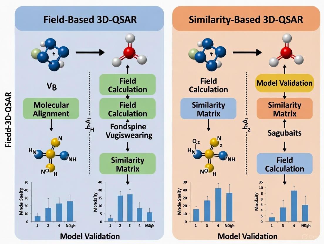
Comparative Molecular Field Analysis (CoMFA), introduced in 1988, was the first and remains the most iconic field-based 3D-QSAR method [2]. Its operational workflow can be broken down into several key stages, as illustrated in the diagram below.
Critical Implementation Steps:
- Molecular Alignment: A set of molecules with known biological activities is aligned in 3D space according to a postulated pharmacophore or a common scaffold. The accuracy of this alignment is arguably the most critical step, as it ensures that the computed fields correspond meaningfully across the dataset [2].
- Grid Generation and Field Calculation: The aligned molecules are placed within a regularly spaced 3D grid. At each grid point, the steric (Lennard-Jones) and electrostatic (Coulombic) interaction energies between a probe atom and each molecule are calculated [3].
- Statistical Correlation via PLS: The vast number of grid-point variables (descriptors) is correlated with the biological activity data using Partial Least Squares (PLS) regression. PLS is adept at handling datasets where the number of variables far exceeds the number of observations and where variables are highly collinear [4] [5].
- Visualization as Contour Maps: The results are interpreted visually through 3D contour maps. These maps highlight regions in space where specific changes in steric or electrostatic properties are predicted to increase or decrease biological activity, providing an intuitive guide for molecular design [3].
Comparative Analysis: Field-Based vs. Similarity-Based 3D-QSAR
While both are 3D-QSAR techniques, field-based and similarity-based approaches differ fundamentally in their underlying principles and descriptors. The table below provides a systematic comparison.
Table 1: Comparison of Field-Based and Similarity-Based 3D-QSAR Approaches
| Feature | Field-Based (CoMFA Paradigm) | Similarity-Based (e.g., LISA, FBSS) |
|---|---|---|
| Core Descriptor | Molecular Interaction Fields (MIFs) - interaction energies with probes [1]. | Global or local molecular similarity indices, often based on shape or pharmacophore overlap [4] [2]. |
| Molecular Representation | Grid-based potential fields surrounding the molecule. | Overlaid structures and their computed similarity to a reference. |
| Descriptor Types | Primarily steric and electrostatic; extended in CoMSIA to hydrophobic and H-bond donor/acceptor fields [3]. | Similarity indices that may segregate regions into "favored similar" and "disfavored similar" potentials [4]. |
| Underlying Calculation | Force-field based (e.g., Coulombic, Lennard-Jones) or Gaussian functions for smoother fields (CoMSIA) [3]. | Similarity metrics (e.g., Carbo index, Petke's formula) computed across molecular alignments [4] [2]. |
| Primary Output | 3D contour maps showing regions where specific properties enhance/diminish activity. | A view of molecular sites permitting favorable changes, often with insight into binding mechanisms [4]. |
| Key Strength | Direct, physically intuitive interpretation of chemical space and interaction requirements. | Can suggest non-obvious alignments and may be less sensitive to alignment artifacts in some cases [2]. |
A key advancement within the field-based paradigm is Comparative Molecular Similarity Indices Analysis (CoMSIA). Developed by Klebe et al., CoMSIA addresses several CoMFA limitations by using a Gaussian function to calculate similarity indices, thereby avoiding the abrupt energy cutoffs of CoMFA and resulting in models that are less sensitive to molecular alignment and grid parameters [3]. Furthermore, CoMSIA typically incorporates a broader set of physicochemical properties, including hydrophobic and hydrogen bond donor/acceptor fields, providing a more holistic view of the interaction landscape [3].
Performance Evaluation: Experimental Data and Comparative Studies
Empirical comparisons are essential for understanding the relative strengths and practical performance of these methodologies.
Case Study: Histamine H3 Receptor Antagonists
A seminal study compared 2D and 3D-QSAR methods for predicting the binding affinities of 58 arylbenzofuran histamine H3 receptor antagonists [5] [6]. The performance was evaluated using statistical metrics like the Mean Absolute Percentage Error (MAPE) and the Standard Deviation of Error of Prediction (SDEP) from cross-validation.
Table 2: Predictive Performance on H3 Receptor Antagonists [5] [6]
| Method | Type | MAPE | SDEP | Key Findings |
|---|---|---|---|---|
| Multiple Linear Regression (MLR) | 2D | 2.9 - 3.6 | 0.31 - 0.36 | Performance was statistically comparable to ANN and superior to the 3D-HASL method. |
| Artificial Neural Network (ANN) | 2D | 2.9 - 3.6 | 0.31 - 0.36 | Equally effective as MLR for this dataset, despite its higher sophistication. |
| HASL (Hypothetical Active Site Lattice) | 3D (Similarity-based) | Not Superior to 2D | Not Superior to 2D | Results were not as good as those obtained by the 2D methods. |
| CoMFA / CoMSIA | 3D (Field-based) | Not reported in this study | Not reported in this study | Commonly provides interpretable 3D contour maps, a key advantage over 2D models. |
This study underscores a critical point: simpler 2D methods can sometimes achieve predictive accuracy on par with or even exceeding that of more complex 3D methods, particularly when the dataset is congeneric. The primary advantage of field-based 3D methods like CoMFA and CoMSIA, therefore, lies not necessarily in superior predictive power for all systems, but in their rich graphical interpretability, which provides direct, visual guidance for molecular design.
Case Study: Sweetness Intensity of Chalcones
A 2025 study on the sweetness intensity of plant-derived chalcones effectively demonstrates the modern application of field-based 3D-QSAR. Researchers used both CoMFA and CoMSIA to decode the structure-sweetness relationship for 25 chalcones [7]. The resulting models were highly informative, revealing that:
- Introducing a negatively charged group at the C2 site of ring A would increase sweetness.
- A positively charged group at the C4 site and a small-volume group with a positive charge at the C6 site were also favorable [7].
The CoMSIA model, in particular, yielded a high cross-validated correlation coefficient (q²) of 0.626, confirming its strong predictive capability. The findings were further validated by molecular docking, illustrating how field-based 3D-QSAR can generate testable, quantitative hypotheses for property optimization even outside traditional pharmaceutical targets [7].
Practical Implementation: Protocols and Reagents
Generic Workflow for a CoMFA/CoMSIA Study
The following protocol outlines the standard steps for conducting a field-based 3D-QSAR analysis.
Protocol 1: Standard Workflow for a Field-Based 3D-QSAR Analysis
- Dataset Curation: Compile a series of molecules (typically 20-100) with consistent and quantitatively measured biological activity (e.g., IC₅₀, Ki).
- Molecular Modeling and Conformational Analysis: Generate reasonable 3D structures for all compounds. For flexible molecules, identify the putative bioactive conformation.
- Molecular Alignment: Superimpose all molecules according to a common scaffold or a hypothesized pharmacophore. This is a critical step that can be done manually or using automated tools like FBSS (Field-Based Similarity Searching) [2].
- Descriptor Calculation (Field Generation):
- Place the aligned molecule set into a 3D grid.
- For CoMFA: Calculate steric (Lennard-Jones) and electrostatic (Coulombic) energies at each grid point using a sp³ carbon and a +1 charge as probes, respectively.
- For CoMSIA: Calculate similarity indices for steric, electrostatic, hydrophobic, and hydrogen bond donor/acceptor fields using a Gaussian function [3].
- Statistical Analysis:
- Use PLS regression to build a model correlating the field descriptors with the biological activity.
- Validate the model using techniques like Leave-One-Out (LOO) cross-validation to obtain a q² value and an external test set to obtain a predictive r² (r²pred) [3].
- Model Interpretation: Analyze the resulting 3D contour maps to identify regions where specific molecular modifications are predicted to enhance activity.
The Scientist's Toolkit: Essential Research Reagents and Software
Table 3: Key Resources for Field-Based 3D-QSAR Research
| Resource / Reagent | Function in 3D-QSAR | Examples / Notes |
|---|---|---|
| Molecular Modeling Suite | Provides the environment for structure building, energy minimization, conformational analysis, and alignment. | Commercial: Schrödinger Suite, MOE. Open-source: Open3DALIGN. |
| 3D-QSAR Software | Performs the core tasks of grid generation, field calculation, PLS analysis, and visualization of contour maps. | Commercial: Built into Schrödinger, MOE. Open-source: Py-CoMSIA (a Python implementation that replicates CoMSIA functionality) [3]. |
| Validated Dataset | Serves as a benchmark for testing new models and methodologies. | The classic steroid benchmark dataset is frequently used for validation [3]. |
| Partial Least Squares (PLS) Algorithm | The statistical engine that correlates the high-dimensional field data with biological activity. | Implemented in all major 3D-QSAR software packages. |
Field-based 3D-QSAR, pioneered by the CoMFA paradigm, provides an indispensable framework for understanding the intricate relationship between a molecule's three-dimensional structure and its biological function. While simpler 2D-QSAR or other similarity-based 3D methods may sometimes achieve comparable predictive accuracy for specific datasets, the defining value of CoMFA and its advanced successor CoMSIA lies in their powerful, visual interpretability. The 3D contour maps generated by these methods transform abstract statistical models into concrete, spatially-resolved design guides, enabling medicinal chemists to make rational decisions about which molecular features to modify and where. The ongoing development of open-source tools, such as Py-CoMSIA, promises to broaden access to these powerful techniques and foster further innovation in the field [3]. As demonstrated by applications ranging from kinase inhibitors to sweetener design, field-based 3D-QSAR remains a vital technology for molecular design and optimization across scientific disciplines.
The concept of molecular similarity represents a foundational principle in computer-aided drug design, underpinning the assumption that structurally similar molecules are likely to exhibit similar biological activities [8]. This molecular similarity principle has driven the development of sophisticated quantitative structure-activity relationship (QSAR) methodologies that translate molecular features into predictive models for biological activity [8]. Among these, three-dimensional QSAR (3D-QSAR) techniques have emerged as powerful tools that consider the spatial orientation of molecules, providing critical insights into the interaction between a ligand and its biological target.
The evolution of 3D-QSAR has progressed through two predominant conceptual frameworks: field-based approaches and similarity-based approaches. Field-based methods, exemplified by Comparative Molecular Field Analysis (CoMFA), characterize molecules by calculating their steric and electrostatic interaction potentials with probe atoms in a 3D grid [9] [10]. While revolutionary, these methods demonstrated sensitivity to molecular alignment and functional parametrization, prompting the development of more advanced similarity-based techniques [9]. Similarity-based approaches, including Comparative Molecular Similarity Indices Analysis (CoMSIA) and emerging Local Molecular Similarity (LISA) methods, employ Gaussian-type distance-dependent functions to evaluate molecular resemblance across multiple physicochemical properties, offering superior handling of molecular alignment and a more comprehensive description of interaction potentials [9] [11].
This guide provides a comprehensive comparison of these methodologies, focusing on their theoretical foundations, practical implementation, predictive performance, and applications in contemporary drug discovery pipelines.
Theoretical Foundations: From Molecular Fields to Similarity Indices
Comparative Molecular Field Analysis (CoMFA): The Field-Based Paradigm
CoMFA operates on the fundamental premise that a molecule's biological activity correlates with its non-covalent interaction fields sampled in three-dimensional space [9] [10]. The methodology involves several systematic steps: first, a set of congeneric molecules is selected and their 3D structures are energy-minimized; second, molecules are aligned according to a hypothesized pharmacophore or bioactive conformation; third, a 3D grid is constructed around the aligned molecules; fourth, steric (Lennard-Jones) and electrostatic (Coulombic) interaction energies between each molecule and a probe atom are calculated at every grid point; finally, Partial Least Squares (PLS) regression correlates these field values with biological activity to generate a predictive model [9]. The results are typically visualized as 3D contour maps indicating regions where specific molecular properties would enhance or diminish biological activity [10].
Despite its widespread adoption and success, CoMFA suffers from several theoretical limitations. The method is highly sensitive to molecular orientation and alignment within the grid, and the Lennard-Jones potential used for steric fields can produce singularities at atomic positions, requiring arbitrary cutoff values [9] [10]. Additionally, the original CoMFA formalism incorporates only steric and electrostatic fields, potentially overlooking other critical interactions such as hydrophobicity and hydrogen bonding that significantly influence ligand-receptor recognition [9].
Comparative Molecular Similarity Indices Analysis (CoMSIA): The Similarity-Based Advancement
CoMSIA was developed to address several limitations inherent in CoMFA. Rather than calculating interaction energies, CoMSIA evaluates similarity indices using a common probe atom at regularly spaced grid points around pre-aligned molecules [9]. The key theoretical advancement lies in the use of a Gaussian-type function for field calculation, which eliminates singularities and provides a "softer" potential that does not require arbitrary cutoff limits [9] [10].
The CoMSIA methodology extends beyond the steric and electrostatic fields of CoMFA to incorporate up to five physicochemical properties: steric, electrostatic, hydrophobic, and hydrogen bond donor and acceptor fields [9]. This comprehensive description of molecular properties allows for a more nuanced understanding of ligand-receptor interactions. The similarity indices (AF) for each property are calculated using the equation:
[ AF(q) = -\sum{i=1}^{n} w{probe,k} w{ik} e^{-\alpha r_{iq}^{2}} ]
where ( w{ik} ) represents the actual value of the physicochemical property k of atom i, ( w{probe,k} ) is the probe value, and ( r_{iq} ) is the mutual distance between the probe atom at grid point q and atom i of the molecule [9]. The exponent ( \alpha ) defines the steepness of the Gaussian function. The resulting contour maps from CoMSIA analyses indicate regions within the molecular region that favor or disfavor specific physicochemical properties, providing more intuitive guidance for molecular optimization [9].
Table 1: Fundamental Differences Between CoMFA and CoMSIA Approaches
| Feature | CoMFA | CoMSIA |
|---|---|---|
| Theoretical Basis | Interaction energy fields | Similarity indices |
| Field Calculation | Lennard-Jones & Coulomb potentials | Gaussian-type distance function |
| Fields Included | Steric, Electrostatic | Steric, Electrostatic, Hydrophobic, H-bond Donor, H-bond Acceptor |
| Alignment Sensitivity | High | Moderate |
| Cutoff Requirements | Required to avoid singularities | Not required |
| Contour Map Interpretation | Regions where fields interact favorably/unfavorably | Regions within ligand space favoring specific properties |
Local Molecular Similarity (LISA) and Evolutionary Methods
Building upon the similarity concept, recent approaches have further refined molecular similarity assessment. Local Molecular Similarity methods focus on specific molecular regions or pharmacophoric features rather than global similarity, potentially offering enhanced selectivity in virtual screening [11]. Evolutionary chemical binding similarity approaches, such as the target-specific ensemble evolutionary chemical binding similarity (TS-ensECBS) model, incorporate machine learning to encode evolutionarily conserved key molecular features required for target-binding into chemical similarity scores [11]. These methods measure the probability that chemical compounds bind to identical or related targets, representing a shift from purely structural similarity to functional similarity based on binding site characteristics [11].
Methodological Comparison: Experimental Protocols and Workflows
Standard CoMSIA Protocol
The implementation of a CoMSIA study follows a well-defined workflow that shares initial steps with CoMFA but diverges in field calculation and analysis [9]:
Dataset Preparation: A series of molecules with known biological activities is compiled. For robust model development, the dataset should be divided into training (typically 80-85%) and test sets (15-20%) [12].
Molecular Modeling and Conformational Analysis: 3D molecular structures are constructed and energy-minimized using molecular mechanics (e.g., MM2) or quantum chemical methods (e.g., AM1). The most likely bioactive conformation is identified for each molecule [9] [6].
Molecular Alignment: This critical step involves superimposing molecules based on a common scaffold, pharmacophoric features, or receptor-active site. The most active compound is often used as a template [9]. For example, in a study of 6-aryl-5-cyano-pyrimidine derivatives as LSD1 inhibitors, molecules were aligned based on their common pyrimidine scaffold [13].
Field Calculation: A 3D grid with typically 2.0 Å spacing is created around the aligned molecules. Similarity indices are calculated for each physicochemical property using a probe atom with specific characteristics: radius 1.0 Å, charge +1, hydrophobicity +1, and hydrogen bond donor and acceptor properties +1 [9].
Statistical Analysis and Model Validation: Partial Least Squares (PLS) regression correlates the similarity indices with biological activity. Model quality is assessed using cross-validated correlation coefficient (q²), conventional correlation coefficient (r²), standard error of estimate (SEE), and F-value [12] [9]. For instance, a CoMSIA model for 6-hydroxybenzothiazole-2-carboxamide derivatives as MAO-B inhibitors demonstrated strong predictive power with q² = 0.569 and r² = 0.915 [12].
CoMSIA Methodology Workflow: This diagram illustrates the standard workflow for CoMSIA model development, highlighting the sequential steps from dataset preparation to predictive application.
Machine Learning-Enhanced CoMSIA Protocols
Recent advances have integrated machine learning (ML) techniques with CoMSIA to address limitations of traditional PLS regression, particularly when handling the high dimensionality of CoMSIA descriptors [14] [15]. A novel ML-enhanced protocol demonstrated superior performance for identifying lipid antioxidant peptides:
Feature Selection: Recursive Feature Elimination (RFE) and SelectFromModel techniques were applied to identify the most relevant CoMSIA descriptors from thousands of initially generated indices [14] [15].
Algorithm Selection and Hyperparameter Tuning: Twenty-four different regression estimators were evaluated, with tree-based models like Gradient Boosting Regression (GBR) showing particular promise. Hyperparameter tuning through GridSearchCV optimized parameters such as learningrate, maxdepth, and n_estimators [14] [15].
Model Validation: The optimized GB-RFE with GBR model (learningrate = 0.01, maxdepth = 2, n_estimators = 500, subsample = 0.5) demonstrated superior performance with RCV² of 0.690, R²test of 0.759, and R² of 0.872 compared to the traditional PLS model (RCV² of 0.653, R²test of 0.575, and R² of 0.755) [14] [15].
This integrated approach effectively mitigated overfitting issues commonly encountered with traditional CoMSIA models and enhanced predictive accuracy for novel compound design [14].
Performance Comparison: Quantitative Analysis of Predictive Accuracy
Direct comparison of CoMFA and CoMSIA methodologies across various therapeutic targets reveals distinct performance patterns that inform method selection for specific applications.
Table 2: Performance Comparison of CoMFA and CoMSIA Across Various Targets
| Therapeutic Target | Compound Series | Best CoMFA Model (q²/r²) | Best CoMSIA Model (q²/r²) | Key Interaction Fields | Reference |
|---|---|---|---|---|---|
| HIV-1 Protease | HOE/BAY-793 analogs | 0.562/0.985 | 0.662/0.989 | Steric, Electrostatic, H-bond Donor | [10] |
| LSD1 Inhibitors | 6-Aryl-5-cyano-pyrimidines | 0.802/0.979 | 0.799/0.982 | Electrostatic, Hydrophobic, H-bond Donor | [13] |
| MAO-B Inhibitors | 6-Hydroxybenzothiazole-2-carboxamides | N/R | 0.569/0.915 | Steric, Electrostatic, Hydrophobic | [12] |
| Lipid Antioxidant Peptides | Tryptophyllin L fragments | N/R | 0.653/0.755 (Traditional PLS) | Steric, Electrostatic, Hydrophobic | [14] |
| Lipid Antioxidant Peptides | Tryptophyllin L fragments | N/R | 0.690/0.872 (ML-Enhanced) | Steric, Electrostatic, Hydrophobic | [14] |
Cross-validated correlation coefficient (q²) and conventional correlation coefficient (r²) values are reported where available. *RCV² and R² values reported for the lipid antioxidant peptide study [14]. N/R = Not Reported.
The quantitative comparisons reveal several important trends. CoMSIA frequently demonstrates comparable or superior predictive performance relative to CoMFA, with the HIV-1 protease inhibitor study showing a notably higher q² value for CoMSIA (0.662) compared to CoMFA (0.562) [10]. The additional physicochemical properties included in CoMSIA (hydrophobicity, hydrogen bonding) often contribute significantly to model quality, as observed in the LSD1 inhibitor study where electrostatic, hydrophobic and H-bond donor fields played crucial roles [13]. Most significantly, the integration of machine learning feature selection and algorithm optimization with CoMSIA descriptors substantially enhanced model predictivity and mitigated overfitting, demonstrating the potential of hybrid approaches [14] [15].
Research Applications and Case Studies
Lipid Antioxidant Peptide Discovery
A comprehensive application of ML-enhanced CoMSIA was demonstrated in the identification of lipid antioxidant peptides from Tryptophyllin L tripeptide fragments [14] [15]. The optimized model identified key molecular features contributing to ferric thiocyanate (FTC) antioxidant activity and screened potential antioxidant tripeptides. Subsequent synthesis and experimental validation confirmed promising activity levels for three peptides: F-P-5Htp (FTC = 4.2 ± 0.12), F-P-W (FTC = 4.4 ± 0.11), and P-5Htp-L (FTC = 1.72 ± 0.15) [14] [15]. This case study highlights the successful translation of computational predictions to experimentally verified bioactive compounds.
Kinase Inhibitor Identification Using Similarity-Based Approaches
The evolutionary chemical binding similarity approach (TS-ensECBS), which shares conceptual foundations with local molecular similarity methods, demonstrated remarkable efficacy in virtual screening for kinase targets [11]. In a blinded validation study, the method identified novel inhibitors for MEK1 and EPHB4 kinases with a success rate of 46.2% (6 out of 13 compounds) for MEK1 and 16.7% (2 out of 12 compounds) for EPHB4 confirmed through in vitro binding assays [11]. Notably, many identified molecules exhibited low structural similarity to known inhibitors, revealing novel scaffolds that would likely have been missed by traditional similarity methods [11].
CNS-Active Agent Optimization
Molecular field-based similarity approaches have also proven valuable in central nervous system drug discovery. A field point analysis of quinoline-based agents with CNS activity assessed their 3D similarity to standard atypical antipsychotics [8]. The compounds demonstrated relatively lower 3D similarity to clozapine but higher similarity to extended chain compounds like ketanserin, ziprasidone, and risperidone [8]. These computational findings aligned with previously reported physicochemical similarity measures and biological activity profiles, supporting the utility of field-based similarity assessments in understanding structure-activity relationships for complex molecular targets [8].
Table 3: Essential Research Reagents and Computational Tools for Similarity-Based 3D-QSAR
| Resource Category | Specific Tools/Software | Key Function | Application in 3D-QSAR | |
|---|---|---|---|---|
| Molecular Modeling | SYBYL/Tripos Force Field, ChemBio3D, Hyperchem | 3D structure construction, energy minimization, conformational analysis | Molecular preparation and optimization prior to alignment | [8] [6] |
| Field Calculation | FieldAlign, Open3DALIGN, in-house Python scripts | Molecular alignment, similarity field calculation, grid generation | Core CoMSIA field computation and descriptor generation | [8] [15] |
| Statistical Analysis | Partial Least Squares (PLS), Scikit-learn (Python) | Regression modeling, feature selection, hyperparameter tuning | Correlation of similarity indices with biological activity | [14] [9] |
| Machine Learning | Gradient Boosting Regression, Random Forest, SVM | Nonlinear pattern recognition, descriptor optimization | Enhanced prediction accuracy and feature selection | [14] [11] |
| Validation Tools | Cross-validation routines, bootstrapping algorithms | Model validation, robustness assessment | Statistical verification of model predictivity | [14] [12] |
| Visualization | PyMOL, VMD, SYBYL contour maps | 3D visualization of contour maps, molecular interactions | Interpretation of favorable/unfavorable molecular regions | [13] [10] |
The evolution from field-based to similarity-based 3D-QSAR approaches represents significant methodological advancement in computational drug design. CoMSIA's Gaussian potential functions, diverse physicochemical fields, and more intuitive contour maps address key limitations of the CoMFA approach while maintaining strong predictive performance. The integration of machine learning for feature selection and model optimization further enhances the utility of similarity-based methods, as demonstrated by the superior performance of ML-enhanced CoMSIA in identifying antioxidant peptides [14] [15].
Future developments in similarity-based 3D-QSAR will likely focus on several promising directions. Dynamic 3D-QSAR approaches that incorporate molecular flexibility and explicit solvation effects may provide more physiologically relevant models [12]. The integration of deep learning architectures for automatic feature extraction from molecular fields could further reduce reliance on expert-driven alignment rules [11]. Additionally, hybrid methods combining ligand-based similarity approaches with structural information from target proteins offer opportunities for enhanced predictive accuracy across diverse chemical classes [11].
As these methodologies continue to evolve, similarity-based 3D-QSAR approaches will remain indispensable tools in the molecular design toolkit, providing critical insights into structure-activity relationships and accelerating the discovery of novel therapeutic agents.
The field of Quantitative Structure-Activity Relationships (QSAR) has fundamentally transformed drug discovery by providing a systematic framework to correlate chemical structure with biological activity. The journey began with classical Hansch analysis in the 1960s, which established the fundamental principle that biological activity correlates with physicochemical properties of chemical substances [16] [17]. This paradigm established that similar compounds typically exhibit similar biological properties, laying the groundwork for computational approaches in medicinal chemistry [16]. For decades, QSAR has served as an indispensable predictive tool in the design of pharmaceuticals and agrochemicals, significantly reducing the trial-and-error factor involved in drug development by facilitating the selection of the most promising candidates for synthesis [17].
The evolution from these early one-dimensional approaches to sophisticated three-dimensional (3D) methods represents one of the most significant advancements in computer-aided drug design. This transition was driven by the recognition that classical QSAR approaches had limited utility for designing new molecules due to their inability to account for the three-dimensional structure of molecules and their interaction with biological targets [17]. This comprehensive review traces this historical progression, comparing the methodological approaches, applications, and predictive capabilities of classical and modern 3D-QSAR techniques within the broader context of field-based versus similarity-based approaches.
The Classical Era: Hansch Analysis and 2D-QSAR
Fundamental Principles and Methodologies
Hansch analysis, pioneered by Corwin Hansch in the 1960s, operates on the principle that biological activity can be correlated with physicochemical properties using linear free-energy relationships [16] [17]. This approach utilizes global molecular descriptors that reduce complex molecular structures to numerical values representing key properties:
- Lipophilicity (logP): Representing the partition coefficient between octanol and water phases
- Electronic properties: Including Hammett constants and dipole moments
- Steric parameters: Such as Taft's steric factor and molar refractivity [16] [17]
In classical QSAR, molecules are described using summary descriptors that do not depend on the molecule's three-dimensional orientation. These one-dimensional or two-dimensional descriptors remain invariant when the molecule is rotated or translated in space, treating molecular structure as essentially flat or feature-based rather than three-dimensional [18]. The developed model typically includes a set of selected variables (descriptors) that are statistically significant and allow insights into the mode of studied interaction, though this approach does not adequately describe ligand-receptor interactions that depend on spatial arrangement [16].
Mathematical Formulation and Application
The classical Hansch approach employs Multiple Linear Regression (MLR) to construct mathematical relationships of the general form:
Activity = f(D₁, D₂, D₃...)
Where D₁, D₂, D₃ represent molecular descriptors encoding specific structural features, including polarizability, electronic properties, and steric parameters [16] [19]. These descriptors encode certain structural features that influence biological activity, with the model providing a statistical correlation between these features and the measured biological endpoint [16].
The methodology follows a structured workflow:
- Calculation of physicochemical descriptors for a series of compounds with known activity
- Selection of the most relevant descriptors using statistical methods
- Development of a linear mathematical model correlating descriptors with biological activity
- Validation using internal and external validation techniques [19]
Table 1: Key Descriptors in Classical Hansch Analysis
| Descriptor Category | Specific Examples | Structural Property Represented |
|---|---|---|
| Lipophilic | logP, π (Hansch constant) | Hydrophobicity, membrane permeability |
| Electronic | σ (Hammett constant), dipole moment, HOMO/LUMO energies | Electron donating/withdrawing effects, molecular reactivity |
| Steric | Molar refractivity, Taft's steric constant, surface area | Molecular size, shape, and bulkiness |
| Structural | Indicator variables, atom counts | Presence/absence of specific functional groups |
The 3D Paradigm Shift: From Flat to Spatial
The Advent of 3D-QSAR
The limitations of classical approaches prompted the development of three-dimensional QSAR methods that explicitly account for molecular shape and interaction fields. The first application of 3D-QSAR technique was proposed in 1988 by Cramer et al. with their program Comparative Molecular Field Analysis (CoMFA) [16] [17]. This revolutionary approach assumed that differences in biological activity correspond to changes in shapes and strengths of non-covalent interaction fields surrounding the molecules [16] [17].
Unlike classical QSAR that treats molecules as collections of global properties, 3D-QSAR considers molecules as three-dimensional objects with specific shapes and interaction potentials. These methods derive descriptors directly from the spatial structure of the molecule, typically quantifying steric fields (representing regions where molecular bulk may clash or accommodate other structures) and electrostatic fields (mapping areas of positive or negative potential) [18]. This fundamental shift from "what groups are present" to "where and how these groups are arranged in space" represented a quantum leap in molecular modeling capabilities.
Key Methodological Differences
The transition from 2D to 3D QSAR introduced several critical methodological distinctions:
- Descriptor Computation: 3D-QSAR involves aligning each molecule within a coordinate grid and computing field values at specific points surrounding it, leading to a much higher dimensional descriptor space than in classical QSAR [18]
- Conformational Dependence: Unlike 2D descriptors that are invariant to conformation, 3D descriptors depend on the molecular conformation and orientation in space
- Alignment Sensitivity: 3D-QSAR methods, particularly CoMFA, are highly sensitive to molecular alignment, requiring careful superposition based on putative bioactive conformations [18]
Table 2: Fundamental Differences Between Classical and 3D QSAR Approaches
| Aspect | Classical (Hansch) QSAR | 3D-QSAR Methods |
|---|---|---|
| Structural Representation | 1D/2D descriptors (logP, molar refractivity) | 3D interaction fields (steric, electrostatic) |
| Descriptor Dimensionality | Low (typically <10 parameters) | High (hundreds to thousands of grid points) |
| Conformational Dependence | None | Critical (requires bioactive conformation) |
| Alignment Requirement | Not applicable | Essential for field-based methods |
| Statistical Methods | MLR, PCA | PLS, G/PLS, ANN |
| Interpretation | Numerical coefficients | 3D contour maps |
| Handling of Structural Diversity | Limited to congeneric series | Accommodates greater diversity |
Modern 3D-QSAR Methodologies: Field-Based vs. Similarity-Based Approaches
Field-Based Methods: CoMFA and Beyond
Comparative Molecular Field Analysis (CoMFA) stands as the pioneering field-based 3D-QSAR approach. The methodology involves placing aligned molecules within a 3D lattice and using a probe atom to calculate steric (Lennard-Jones) and electrostatic (Coulombic) interaction energies at each grid point [16] [18]. The collection of these field values forms a fingerprint-like descriptor for the molecule's 3D shape and electrostatic profile, which is then correlated with biological activity using Partial Least Squares (PLS) regression [18].
Comparative Molecular Similarity Indices Analysis (CoMSIA) extends CoMFA by using Gaussian-type functions to evaluate steric, electrostatic, hydrophobic, and hydrogen-bonding fields [18]. This approach smooths out abrupt field changes near molecular surfaces and enhances interpretability, especially across structurally diverse compounds. While CoMFA is highly sensitive to alignment quality, CoMSIA offers more tolerance to minor misalignments, thereby expanding its applicability [18].
A recent study on MAO-B inhibitors demonstrated the power of CoMSIA, where the developed model exhibited excellent predictive ability with a q² value of 0.569 and r² value of 0.915, successfully guiding the design of novel neuroprotective agents [20].
Similarity-Based Approaches and Local Methods
As alternatives to field-based approaches, similarity-based methods have emerged that focus on molecular similarity indices rather than interaction fields. The Local Indices for Similarity Analysis (LISA) approach breaks global molecular similarity into local similarity at each grid point surrounding molecules, using these as QSAR descriptors [4]. This method segregates regions into "equivalent," "favored similar," and "disfavored similar" potentials with respect to a reference molecule, providing insights into binding mechanisms and allowing fine-tuning of molecules at the local level to improve activity [4].
Similarity-based approaches offer distinct advantages in their straightforward graphical interpretation and ability to handle structurally diverse datasets without stringent alignment requirements. The outcome of these models corroborates well with literature data and provides medicinal chemists with intuitive guidance for molecular optimization [4].
Table 3: Comparison of Major 3D-QSAR Methodologies
| Method | Descriptor Basis | Fields/Indices Calculated | Alignment Sensitivity | Key Advantages |
|---|---|---|---|---|
| CoMFA | Steric/electrostatic interaction energies | Lennard-Jones, Coulomb | High | Established method, intuitive fields |
| CoMSIA | Similarity indices using Gaussian functions | Steric, electrostatic, hydrophobic, H-bond donor/acceptor | Moderate | Broader field types, smoother sampling |
| LISA | Local similarity indices | Shape, electrostatic similarity | Moderate | Direct similarity comparison, local optimization guidance |
| HASL | Composite lattice from 3D grids | Multipoint pharmacophore patterns | Low to moderate | Handles conformational flexibility |
| ML-Based 3D-QSAR | Shape, color, electrostatic featurizations | ROCS shape, EON electrostatics | Variable (alignment-free options) | Error estimation, confidence predictions [21] |
Experimental Protocols and Methodological Workflows
Building a Robust 3D-QSAR Model
The construction of a reliable 3D-QSAR model follows a systematic workflow with critical steps at each phase:
Data Collection and Preparation: Assembling a dataset of compounds with experimentally determined biological activities (IC₅₀, EC₅₀, Kᵢ) measured under uniform conditions is paramount. The integrity of this dataset directly impacts model quality, requiring structurally related yet sufficiently diverse molecules to capture meaningful structure-activity relationships [18].
Molecular Modeling and Conformation Optimization: 2D structures are converted to 3D coordinates using cheminformatics tools like RDKit or Sybyl, followed by geometry optimization using molecular mechanics (UFF) or quantum mechanical methods to ensure realistic, low-energy conformations [18]. For the classic nano-QSAR approach, optimal geometries of investigated fullerene derivatives were obtained applying Density Functional Theory (DFT) with the hybrid meta exchange-correlation functional M06-2X and the 6-31G(d,p) basis set [16].
Molecular Alignment: This critical step involves superimposing all molecules in a shared 3D reference frame reflecting putative bioactive conformations. Approaches include:
- Bemis-Murcko Scaffold: Removing side chains and retaining ring systems and linkers
- Maximum Common Substructure (MCS): Identifying largest shared substructure
- Pharmacophore-based alignment: Using common chemical features [18]
Descriptor Calculation and Variable Selection: For CoMFA, a lattice of grid points surrounds the molecules where steric and electrostatic interaction energies are calculated using probe atoms [18]. With modern machine learning approaches, featurization using shape (from ROCS) and electrostatics (from EON) provides comprehensive 3D molecular representations [21]. Genetic algorithms are often employed for variable selection to identify the most relevant descriptors [16] [19].
Model Building and Validation: PLS regression correlates field values with biological activities. Robust validation includes:
The Scientist's Toolkit: Essential Research Reagents and Solutions
Table 4: Essential Computational Tools for 3D-QSAR Research
| Tool Category | Specific Software/Solutions | Primary Function |
|---|---|---|
| Molecular Modeling | Sybyl-X, Schrodinger Suite, HyperChem | 3D structure generation, optimization, and visualization |
| Quantum Chemistry | Gaussian 09, GAMESS, ORCA | Quantum mechanical calculations, orbital energies, accurate geometry optimization |
| Cheminformatics | RDKit, OpenBabel, Dragon | Descriptor calculation, file format conversion, structural analysis |
| Alignment Tools | ROCS, Phase | Molecular superposition using shape or pharmacophore features |
| 3D-QSAR Specific | CoMFA, CoMSIA (in Sybyl), HASL | Field calculation, similarity analysis, model building |
| Statistical Analysis | QSARINS, MATLAB, R | MLR, PLS, genetic algorithm variable selection |
| Machine Learning | Python Scikit-learn, TensorFlow, Orion | Advanced pattern recognition, model building with error estimation [21] |
Comparative Performance and Applications
Quantitative Performance Metrics
Direct comparisons between classical and 3D-QSAR approaches reveal distinct performance characteristics. In a study comparing different 2D and 3D-QSAR methods for predicting histamine H3 receptor antagonist activity, 3D methods generally demonstrated superior predictive capability for structurally diverse compounds, while well-parameterized 2D models performed adequately for congeneric series [6].
A recent 3D-QSAR study on MAO-B inhibitors demonstrated impressive statistical results with a CoMSIA model exhibiting q² = 0.569, r² = 0.915, SEE = 0.109, and F value = 52.714 [20]. Similarly, modern machine learning-enhanced 3D-QSAR approaches show performance on-par with or better than published methods, with the additional advantage of providing prediction error estimates to help users identify the right compounds for the right reasons [21].
Application Case Studies
The evolution from Hansch analysis to 3D methods has expanded QSAR applications across multiple domains:
Drug Discovery: 3D-QSAR has become indispensable in lead optimization campaigns, successfully guiding the design of HIV-1 protease inhibitors [16], MAO-B inhibitors for neurodegenerative diseases [20], and NF-κB inhibitors for inflammatory conditions and cancer [19]
Toxicity Prediction: Nano-QSAR approaches have been developed to investigate nanoparticle toxicity and environmental health effects, with 3D methods providing insights into interaction mechanisms [16]
Materials Science: QSAR approaches have been applied to predict corrosion inhibition efficiency, with recent studies demonstrating that 3D descriptors combined with machine learning models like XGBoost achieve superior predictive performance (R² = 0.94-0.96 for training sets) [22]
Environmental Chemistry: Prediction of aquatic toxicity, pesticide effects, and environmental fate of chemicals [19]
Current Trends and Future Perspectives
The field of QSAR continues to evolve with emerging trends shaping its future development. Integration of machine learning with 3D-QSAR represents perhaps the most significant advancement, with models featurized using shape, color, and electrostatic properties demonstrating enhanced predictive capability [21]. These approaches leverage the full 3D similarity of molecules while providing confidence estimates for predictions.
Ultra-large virtual screening capabilities now enable researchers to screen billions of compounds, with 3D-QSAR models providing rapid prioritization of candidates for more computationally intensive methods like free energy calculations [23] [21]. The synergy between rapid 3D-QSAR screening and detailed molecular dynamics simulations creates a powerful multi-tiered approach to drug discovery [20].
Future developments will likely focus on dynamic 3D-QSAR approaches that account for protein flexibility and binding site adaptations, moving beyond the static ligand-receptor interaction paradigm. Additionally, the integration of deep learning architectures with 3D molecular representations promises to further enhance predictive accuracy while reducing dependence on precise molecular alignment [23].
The historical evolution from Hansch analysis to modern 3D-QSAR methods represents a remarkable journey of increasing molecular representation complexity and predictive capability. While classical QSAR approaches established the fundamental principle that biological activity correlates with molecular structure, their limitation to global descriptors restricted their utility for detailed molecular design.
The advent of 3D-QSAR methodologies addressed this limitation by explicitly incorporating spatial and electronic properties, enabling medicinal chemists to visualize and optimize molecular interactions with biological targets. The distinction between field-based approaches like CoMFA/CoMSIA and similarity-based methods like LISA provides researchers with complementary tools for addressing different challenges in molecular design.
As the field continues to evolve, the integration of machine learning with 3D structural information promises to further enhance predictive accuracy and practical utility. This ongoing innovation ensures that QSAR methodologies will remain indispensable tools in drug discovery and molecular design, building upon the foundation established by Hansch over half a century ago while embracing the computational power and theoretical advances of the modern era.
In the field of computer-aided drug design, Three-Dimensional Quantitative Structure-Activity Relationship (3D-QSAR) methods are pivotal for correlating the biological activity of compounds with their spatial characteristics. Two dominant paradigms have emerged: the interaction energy fields approach and the Gaussian similarity indices methodology. While both aim to predict and optimize compound activity, their underlying principles and operational frameworks differ significantly. Interaction energy fields, exemplified by methods like Comparative Molecular Field Analysis (CoMFA), directly compute physico-chemical potential energies around molecules [24]. In contrast, Gaussian similarity indices, central to techniques like Comparative Molecular Similarity Indices Analysis (CoMSIA), employ probabilistic functions to measure molecular resemblance [25] [26]. This guide provides an objective comparison of these strategies, detailing their performance, supported by experimental data and practical implementation protocols.
Theoretical Foundations and Methodological Principles
Core Conceptual Frameworks
The fundamental distinction between these approaches lies in how they represent and quantify molecular environments.
Interaction Energy Fields are rooted in classical molecular mechanics [24]. This approach posits that a biological receptor perceives a ligand not as atoms and bonds, but as a shape carrying complex forces, predominantly steric and electrostatic potentials. The method involves placing a target molecule within a 3D lattice and using a probe atom (e.g., an sp³ carbon with a +1 charge for electrostatic fields) to calculate the interaction energy at each grid point using potentials like Coulomb's law (electrostatic) and Lennard-Jones (steric) [24]. The resulting data represents a direct mapping of the Molecular Interaction Fields (MIFs), which can be visualized as iso-potential surfaces to identify favorable and unfavorable interaction regions around the molecule.
Gaussian Similarity Indices, used in methods like CoMSIA, abandon the direct calculation of harsh potential energies [25]. Instead, they describe molecular properties using Gaussian-type functions for distance dependence [27] [26]. This approach calculates the similarity of molecules in a set to a common probe placed at grid points, using a Gaussian function to avoid singularities and extreme values inherent in classical potential functions. CoMSIA typically extends beyond steric and electrostatic fields to include hydrogen bond donor, hydrogen bond acceptor, and hydrophobic fields, providing a more nuanced description of interaction potential [25] [26].
Mathematical Underpinnings
The mathematical representation highlights their core differences:
- Interaction Energy Fields (CoMFA): The steric energy ( E{steric} ) is often described by a Lennard-Jones potential ( E = \frac{A}{r^{12}} - \frac{B}{r^6} ), and electrostatic energy ( E{electrostatic} ) by Coulomb's law ( E = \frac{q1 q2}{\epsilon r} ), where ( r ) is the distance from a grid point to an atom, and ( q ) is atomic charge [24].
- Gaussian Similarity Indices (CoMSIA): The similarity index ( AF ) for a property ( F ) at grid point ( q ) is calculated as ( AF(q) = -\sumi \omega{probe} \omega{ik} e^{-\alpha r{iq}^2} ), where ( \omega{ik} ) is the actual value of the property for atom ( i ), ( r{iq} ) is the distance between grid point ( q ) and atom ( i ), and ( \alpha ) is an attenuation factor [27] [26]. This Gaussian function ensures the similarity indices decay smoothly with distance.
Table 1: Core Conceptual Differences Between the Two Approaches
| Feature | Interaction Energy Fields (e.g., CoMFA) | Gaussian Similarity Indices (e.g., CoMSIA) |
|---|---|---|
| Fundamental Principle | Calculation of physico-chemical potential energies | Measurement of molecular similarity using Gaussian functions |
| Distance Dependence | Inverse power laws (e.g., (1/r), (1/r^{12})) | Exponential decay ((e^{-\alpha r^2})) |
| Handling of Singularities | Prone to extreme values near van der Waals surfaces | Avoided due to Gaussian function properties |
| Primary Descriptors | Steric and Electrostatic fields | Steric, Electrostatic, Hydrophobic, H-bond Donor, H-bond Acceptor fields |
| Probe Usage | Single-atom probe to measure energy | Common probe to measure similarity indices |
| Visualization | Direct interpretation of potential energy contours | Interpretation of similarity and dissimilarity regions |
Experimental Protocols and Workflow Implementation
Standardized Workflow for 3D-QSAR Model Development
The following diagram illustrates the general workflow for developing a 3D-QSAR model, highlighting steps where the two methodologies diverge.
Detailed Methodological Protocols
Protocol for Interaction Energy Fields (CoMFA) [24] [25]:
- Molecular Alignment: Align training set molecules based on a presumed bioactive conformation, using a common scaffold or pharmacophore hypothesis.
- Grid Generation: Embed the aligned molecules in a 3D grid with a typical spacing of 1.0–2.0 Å, ensuring all molecules are contained.
- Interaction Energy Calculation:
- Steric Field: Use an sp³ carbon probe with a van der Waals radius of 1.52 Å and a typical energy cutoff of 30 kcal/mol. Calculate using a 6-12 Lennard-Jones potential.
- Electrostatic Field: Use a +1.0 charged sp³ carbon probe. Calculate using Coulomb's law with a distance-dependent dielectric constant (e.g., ε = 1r).
- Data Reduction and PLS Analysis: Use Partial Least Squares (PLS) regression to correlate the energy field values with biological activity. Apply cross-validation (e.g., leave-one-out) to determine the optimal number of components and avoid overfitting.
Protocol for Gaussian Similarity Indices (CoMSIA) [25] [26]:
- Molecular Alignment and Grid Generation: Perform identical to the CoMFA protocol.
- Similarity Indices Calculation: For each molecule, calculate similarity indices at all grid points for five property fields: steric, electrostatic, hydrophobic, hydrogen bond donor, and hydrogen bond acceptor.
- Use a Gaussian function with a default attenuation factor ( \alpha ) of 0.3.
- The hydrophobic field is derived from atom-based parameters (e.g., Crippen log P fragments). Hydrogen bond donor and acceptor fields use appropriate probe atoms.
- Statistical Analysis: Perform PLS regression on the similarity indices. The smoother nature of the CoMSIA fields often requires a different column filtering value than CoMFA.
Performance Comparison and Experimental Data
Quantitative Performance Metrics
Independent studies across different biological targets provide objective performance comparisons.
Table 2: Experimental Performance Comparison from Literature Case Studies
| Study Context | Method | Statistical Metrics | Key Performance Findings | Reference |
|---|---|---|---|---|
| Antitumor Diaryl-sulfonylureas (28 compounds) | CoMFA | q² = 0.653, r² = 0.955 | Superior statistical correlation, best model in study | [25] |
| CoMSIA | q² = 0.638, r² = 0.934 | Comparable, strong performance | [25] | |
| Lipid Antioxidant Peptides (FTC Dataset, 197 peptides) | CoMSIA (Traditional PLS) | R²CV = 0.653, R²test = 0.575 | Baseline performance with linear PLS | [26] |
| CoMSIA (ML-Enhanced, GBR) | R²CV = 0.690, R²test = 0.759 | Machine learning integration significantly boosted predictivity | [26] | |
| Quantum Mechanical MIFs (9 diverse datasets) | QM-Based MIFs | N/A | Average performance superior to force-field (FF) MIFs; performance equal or better in all datasets | [28] |
Qualitative Comparative Analysis
- Interpretability and Visualization: CoMFA contour maps directly indicate regions where increased steric bulk or positive/negative charge is favorable/unfavorable for activity [24]. CoMSIA maps, due to the Gaussian basis, are often considered less harsh and may more clearly define favorable regions for specific interactions like hydrogen bonding or hydrophobicity [25].
- Robustness to Alignment: The Gaussian similarity indices in CoMSIA are less sensitive to small changes in molecular alignment within the grid because the functions decay smoothly. CoMFA's classical potentials can produce large energy changes with small atomic displacements, especially near the van der Waals surface [25] [26].
- Application Scope: CoMSIA's inclusion of additional fields (hydrophobic, H-bond) can be advantageous for targets where these interactions are critical, providing a more holistic view of the binding landscape [25] [26].
The Scientist's Toolkit: Essential Research Reagents and Software
Table 3: Key Research Solutions for 3D-QSAR Studies
| Tool / Reagent / Software | Primary Function | Relevance to Field-Based vs. Similarity-Based QSAR |
|---|---|---|
| SYBYL (Tripos) | Commercial molecular modeling suite | Historically the platform where CoMFA and CoMSIA were first implemented and standardized [25]. |
| GRID | Software for calculating MIFs | Pioneering structure-based approach for mapping interaction hotspots with diverse probes, foundational to the field concept [24]. |
| Python with RDKit/Scikit-learn | Open-source cheminformatics and ML | Enables custom implementation of descriptors (e.g., USRCAT) and integration of ML algorithms for model enhancement [27] [26]. |
| OPLS_2005 Force Field | Force field for molecular dynamics | Used for molecular geometry optimization and charge calculation, providing input for both CoMFA and CoMSIA studies [26]. |
| Gasteiger-Hückel Charges | Empirical method for partial atomic charge calculation | A common charge calculation method used to derive the electrostatic fields in CoMFA and CoMSIA models [26]. |
| Ultrafast Shape Recognition (USR) | Alignment-free shape similarity method | Represents a class of Gaussian-overlay based shape descriptors used for fast virtual screening, related to the similarity philosophy [27]. |
Integrated Applications and Future Directions
The combination of both field-based and similarity-based concepts with modern computational techniques represents the future of 3D-QSAR.
- Integration with Machine Learning: As demonstrated with the FTC dataset, replacing traditional PLS with machine learning algorithms like Gradient Boosting Regression (GBR) can significantly improve the predictivity of CoMSIA models, overcoming limitations of linear regression [26]. This synergy allows the rich descriptor sets of 3D-QSAR to be leveraged by more powerful, non-linear fitters.
- Evolution to Quantum Mechanical Fields: A significant shift involves moving from classical force fields to Quantum Mechanical (QM)-based Molecular Interaction Fields [28]. QM-MIFs do not suffer from the fixed atom-centered charge approximation and provide a more accurate description of electron density and polarization effects. Studies show that QMFA models consistently perform equal to or better than conventional force-field-based models [28].
- Hybrid Screening Approaches: Effective virtual screening often combines the strengths of multiple methods. For instance, a workflow might use a fast chemical binding similarity method for initial filtering, followed by more computationally intensive 3D-QSAR pharmacophore or molecular docking studies for refined prediction [11]. This leverages the speed of similarity-based screening and the detailed insight of field-based and structure-based methods.
Implementation and Use Cases: Applying Field and Similarity Methods in Drug Design
In the realm of three-dimensional quantitative structure-activity relationship (3D-QSAR) modeling, the computational workflow of molecular alignment, grid generation, and field calculation forms the essential foundation for predicting biological activity based on molecular structure. These steps transform 3D molecular structures into quantitative descriptors that can be correlated with biological endpoints. Within the broader thesis of comparing field-based and similarity-based 3D-QSAR approaches, the execution of these workflow stages fundamentally diverges, leading to distinct advantages and limitations for each paradigm. Field-based methods like CoMFA (Comparative Molecular Field Analysis) and CoMSIA (Comparative Molecular Similarity Indices Analysis) rely heavily on precise molecular alignment to compute interaction energies, while modern similarity-based approaches often leverage alignment-independent descriptors or consensus models to predict binding affinity. This guide objectively breaks down these critical workflow components, supported by experimental data and comparative performance metrics.
Core Workflow Components and Comparative Analysis
The process of building a 3D-QSAR model follows a defined sequence, with methodological choices at each stage directly influencing the model's predictive performance and interpretability.
Molecular Alignment: The Conformational Foundation
Molecular alignment, or superimposition, aims to position all molecules in a shared 3D space in a manner that reflects their putative bioactive orientation. This is one of the most critical and challenging steps, especially for alignment-dependent methods [18].
- Objective: To ensure that the computed molecular descriptors correspond to equivalent spatial regions relative to a common reference, typically a known active compound or a shared pharmacophoric core [18].
Methodologies:
- Field-Based Workflow: Requires a rigorous, often manual or algorithmically complex, alignment procedure. Common techniques include scaffold-based alignment using the Bemis-Murcko framework or substructure-based alignment via the Maximum Common Substructure (MCS) [18]. The underlying assumption is that all compounds share a similar binding mode to the target protein.
- Similarity-Based Workflow: Employs strategies to minimize or bypass alignment sensitivity. For instance, the topomer approach generates a single, canonical conformation and alignment based solely on a molecule's 2D topology and a predefined fragmentation scheme, making the process fully automated and objective [29]. Other modern implementations may use consensus models that aggregate predictions from multiple alignments [30].
Experimental Protocol: A standardized protocol for field-based alignment involves:
- 3D Structure Generation: Convert 2D structures to 2D using tools like RDKit or Sybyl, followed by geometry optimization with molecular mechanics (e.g., UFF) or quantum mechanical methods [18].
- Template Selection: Identify a high-affinity ligand or a rigid core structure common to the dataset.
- Superimposition: Align all molecules to the template based on atomic correspondences of the shared scaffold or pharmacophoric features using molecular modeling software [18] [20].
Impact of Bioactive Conformations: Studies comparing 2D and 3D descriptors using bioactive conformations (from protein-ligand crystal structures) found that combining 2D and 3D descriptors often yielded more significant models, as they encode complementary molecular properties [31]. Interestingly, research on androgen receptor binders demonstrated that models using simple, non-energy-minimized 2D->3D conformations (directly converted from databases like ChemSpider) could achieve predictive performance (R²Test = 0.61) superior to models using energy-minimized or template-aligned conformations, and in a fraction of the computational time [32].
The following diagram illustrates the key decision points and outcomes in the molecular alignment workflow.
Grid Generation: Defining the Calculational Space
Once molecules are aligned, a 3D grid is constructed to encompass the entire set of aligned molecules. This grid provides the points at which molecular fields will be calculated [18].
- Objective: To create a systematic lattice of points in 3D space that serves as a common framework for sampling and comparing molecular properties across the entire dataset [3].
Methodologies:
- The grid is typically defined by its bounding box (extending beyond the molecular dimensions by a margin of 4-6 Å) and its resolution (spacing between grid points, commonly 1-2 Å) [3].
- This step is largely consistent across field-based and similarity-based methods that rely on 3D grids. The key difference lies in how the grid points are utilized in the subsequent field calculation step.
Experimental Protocol:
- Calculate the spatial extent (min/max coordinates) of all aligned molecules.
- Extend the bounding box by a defined padding (e.g., 4.0 Å) in all directions to ensure the grid encompasses the molecules and their potential interaction volumes.
- Define the grid spacing (e.g., 1.0 Å or 2.0 Å). A finer grid yields more descriptors and higher resolution but increases computational cost and the risk of overfitting [18] [3].
Field Calculation: The Source of Descriptors
This is the stage where field-based and similarity-based methodologies fundamentally diverge in how they characterize molecules.
Objective: To compute numerical values at each grid point that describe the steric, electrostatic, and other physicochemical properties of the molecules [18] [3].
Methodologies and Experimental Protocols:
Field-Based Descriptors (CoMFA/CoMSIA):
- CoMFA: Uses a probe atom (e.g., sp³ carbon with +1 charge) to calculate steric (Lennard-Jones potential) and electrostatic (Coulomb potential) interaction energies at every grid point [18] [33]. A key limitation is the occurrence of abrupt energy changes near the molecular surface.
- CoMSIA: Introduces a Gaussian function to calculate similarity indices, avoiding singularities and making fields less sensitive to small alignment variations. It calculates five fields: steric, electrostatic, hydrophobic, hydrogen bond donor, and hydrogen bond acceptor [3]. The use of a Gaussian function (with an attenuation factor, typically α=0.3) ensures smooth, continuous fields [3].
Similarity-Based Descriptors:
- Methods like OpenEye's 3D-QSAR use descriptors derived from molecular similarity tools, such as shape (ROCS) and electrostatic (EON) comparisons, rather than interaction energy probes [30].
- Predictions are often generated as a consensus from multiple models employing different similarity descriptors and machine learning techniques, enhancing robustness [30].
- The topomer approach leverages the automated alignment to generate CoMFA-like fields, but its accuracy is attributed to focusing field differences only on grid points adjacent to structural changes, minimizing noise from uncertain binding geometry effects [29].
The table below summarizes a quantitative performance comparison of different 3D-QSAR approaches based on various experimental studies.
Table 1: Comparative Performance of 3D-QSAR Methodologies in Practical Applications
| Methodology | Dataset / Application | Performance Metrics | Key Findings |
|---|---|---|---|
| CoMSIA (Field-Based) [20] | 6-hydroxybenzothiazole-2-carboxamide derivatives (MAO-B inhibition) | q² = 0.569, r² = 0.915 (model); Successful prediction of novel derivative 31.j3 with high docking score and stable MD simulation. | Demonstrated high internal consistency and predictive power for designing novel, potent inhibitors. |
| XGBoost with 2D/3D Descriptors [22] | Pyrazole derivatives (corrosion inhibition) | Training set R² = 0.96 (2D), 0.94 (3D); Test set R² = 0.75 (2D), 0.85 (3D); RMSE < 2.84. | Machine learning on 2D/3D descriptors can yield strong predictive ability, with 3D descriptors showing better test set performance. |
| Topomer CoMFA (Similarity-Based) [29] | 140 structures across 4 industrial drug discovery projects (prospective testing) | Average pIC50 prediction error = 0.5. | Unprecedented prediction accuracy in real-world prospective applications, attributed to reduced noise from binding geometry ambiguities. |
| 2D->3D Conformation (Alignment-Independent 3D-SDAR) [32] | 146 androgen receptor binders | R²Test = 0.61 (vs. 0.56-0.61 for other conformations). | Achieved superior predictive accuracy with minimal computational overhead, suggesting utility for large datasets and rigid targets. |
The Scientist's Toolkit: Essential Research Reagents and Software
Successful execution of 3D-QSAR workflows relies on a suite of specialized software tools and computational resources.
Table 2: Essential Tools for 3D-QSAR Research
| Tool / Resource | Type | Primary Function in Workflow | Examples / Notes |
|---|---|---|---|
| Molecular Modeling Suites | Software Platform | Integrated environment for structure building, optimization, alignment, and QSAR analysis. | Schrödinger, Molecular Operating Environment (MOE) (commercial); Sybyl (legacy, discontinued) [3]. |
| Cheminformatics Libraries | Programming Library | Scriptable molecular manipulation, descriptor calculation, and model building. | RDKit (open-source, used in Py-CoMSIA [3]), NumPy. |
| 3D-QSAR Specialized Tools | Specialized Software | Perform specific CoMFA/CoMSIA or similarity-based calculations. | OpenEye's 3D-QSAR (similarity-based, consensus modeling [30]), Py-CoMSIA (open-source CoMSIA implementation [3]). |
| Conformational Generators | Algorithm/Tool | Generate low-energy or bio-active 3D conformations from 2D structures. | Tools within RDKit, Concord (used in topomer generation [29]). |
| Validation & Analysis Tools | Software/Statistical | Model validation, statistical analysis, and visualization of contour maps. | Built-in PLS and cross-validation in QSAR software; PyVista for visualizations in Py-CoMSIA [3]. |
The workflows for molecular alignment, grid generation, and field calculation are not merely procedural steps but embody the core philosophical differences between field-based and similarity-based 3D-QSAR approaches. Field-based methods like CoMSIA offer high interpretability through detailed contour maps but are often gated by the challenge of achieving a correct, bioactive molecular alignment. In contrast, similarity-based and alignment-independent strategies, such as topomer CoMFA or methods using simple 2D->3D conformations, prioritize predictive robustness, automation, and objectivity, often with remarkable success in real-world drug discovery applications [29] [32] [30]. The choice between them depends on the project's specific needs: when a reliable alignment is achievable, field-based methods provide deep insight; for high-throughput prediction or when alignment is uncertain, modern similarity-based and automated approaches offer a powerful and increasingly accurate alternative. The emergence of open-source tools like Py-CoMSIA is making these advanced methodologies more accessible, promising further innovation in the field [3].
In modern drug discovery, three-dimensional quantitative structure-activity relationship (3D-QSAR) modeling represents a pivotal methodology for understanding how the structural features of molecules influence their biological activity. Unlike traditional 2D-QSAR that utilizes numerical descriptors invariant to molecular conformation, 3D-QSAR methods consider molecules as three-dimensional objects with specific shapes and interaction potentials distributed in space [18]. Among 3D-QSAR approaches, a fundamental distinction exists between field-based and similarity-based methods, each with distinct theoretical foundations and practical applications.
Field-based descriptors are founded on the principle that a biological receptor "perceives" a ligand not as a collection of atoms, but as a composite shape with associated molecular forces [24]. These forces—steric, electrostatic, hydrophobic, and hydrogen-bonding potentials—are systematically mapped in the space surrounding molecules to create quantitative descriptors that can be correlated with biological activity. The most established field-based techniques include Comparative Molecular Field Analysis (CoMFA) and Comparative Molecular Similarity Indices Analysis (CoMSIA), which have become indispensable tools in rational drug design [34] [3].
This guide provides a comprehensive comparison of these field-based descriptors, detailing their theoretical foundations, methodological implementation, performance characteristics, and practical applications in contemporary drug discovery research.
Theoretical Foundations and Molecular Field Types
Field-based 3D-QSAR methods operate on the principle that molecular binding is inherently three-dimensional and driven by complementary interactions between a ligand and its receptor [24]. The receptor does not recognize ligands as sets of atoms and bonds, but rather as shapes carrying complex force fields. These interaction fields are quantified using the probe concept, where specific chemical groups are used to measure interaction potentials at numerous points in the space surrounding each molecule [24].
Core Field Descriptors in 3D-QSAR
Table 1: Fundamental Field-Based Descriptors in 3D-QSAR
| Field Type | Physical Basis | Probe Types Used | Computational Function | Biological Significance |
|---|---|---|---|---|
| Steric | van der Waals forces | Carbon sp³ atom | Lennard-Jones potential: ( V_{LJ} = 4\varepsilon[(\frac{\sigma}{r})^{12} - (\frac{\sigma}{r})^6] ) | Molecular shape complementarity, bulk tolerance/clashes [34] [24] |
| Electrostatic | Coulombic interactions | Charged atom (+1 typically) | Coulomb's law: ( E = \frac{q1 q2}{4\pi\varepsilon r} ) | Ion-ion, ion-dipole, dipole-dipole interactions [34] [24] |
| Hydrophobic | Hydrophobic effect | Hypothetical hydrophobic probe | Gaussian-type distance-dependent function | Driven by entropic effects, crucial for membrane permeability and binding [3] |
| Hydrogen-Bond Donor | Directional H-bonding | Hydrogen atom or H-bond donor group | Gaussian function | Specificity in molecular recognition [3] |
| Hydrogen-Bond Acceptor | Directional H-bonding | Oxygen atom or H-bond acceptor group | Gaussian function | Binding affinity and selectivity [3] |
The steric field describes repulsive and attractive van der Waals forces, calculated using the Lennard-Jones potential [34]. At short distances, strong repulsion occurs due to electron cloud overlap, while weaker attractive dispersion forces operate at longer ranges [24]. The electrostatic field, governed by Coulomb's law, represents charge-charge interactions that operate over longer distances and often guide initial ligand approach to the binding site [34] [24].
Hydrophobic fields quantify the entropically driven tendency of nonpolar surfaces to associate in aqueous environments, while hydrogen-bonding fields map the direction-specific potentials for forming hydrogen bond interactions [3]. Compared to CoMFA, which primarily focuses on steric and electrostatic fields, CoMSIA incorporates additional descriptors including hydrophobic and hydrogen-bonding fields, providing a more comprehensive representation of molecular interactions [3].
Methodological Implementation: From Theory to Practice
The implementation of field-based 3D-QSAR models follows a systematic workflow with multiple critical stages where methodological decisions significantly impact model quality and predictive power.
Experimental Workflow for Field-Based 3D-QSAR
The diagram below illustrates the standard workflow for developing field-based 3D-QSAR models:
Critical Methodological Considerations
Molecular Alignment Strategies
Molecular alignment constitutes perhaps the most critical step in alignment-dependent 3D-QSAR methods like CoMFA [18]. The objective is to superimpose all molecules in a shared 3D reference frame that reflects their putative bioactive conformations. Common approaches include:
- Atom-based superimposition: Direct atom-to-atom pairing between molecules based on common substructures [34]
- Maximum Common Substructure (MCS): Identification of the largest shared substructure among a set of molecules [18]
- Pharmacophore-based alignment: Superimposition based on key pharmacophoric features
- Docking-derived alignment: Using molecular docking poses to define alignment [35]
The alignment assumption presumes all compounds share a similar binding mode. Inaccurate alignment introduces inconsistencies in descriptor calculations that undermine the entire modeling process [18].
Field Calculation Methods
Field calculation approaches differ significantly between CoMFA and CoMSIA:
CoMFA (Comparative Molecular Field Analysis) employs a lattice grid with typically 2Å spacing that surrounds the aligned molecules [34]. At each grid point, steric (Lennard-Jones potential) and electrostatic (Coulombic) fields are calculated using probe atoms [34]. A significant limitation is the occurrence of abrupt field changes near molecular surfaces, which can introduce artifacts [3].
CoMSIA (Comparative Molecular Similarity Indices Analysis) introduces a Gaussian-type function to calculate similarity indices, generating continuous molecular similarity maps for all five field types [3]. This approach eliminates sharp cutoffs and makes CoMSIA models less sensitive to molecular alignment and grid parameters compared to CoMFA [3].
Performance Comparison: Field-Based vs. Similarity-Based Approaches
The comparative performance of field-based 3D-QSAR methods can be evaluated through both statistical metrics and practical applicability across different research scenarios.
Quantitative Performance Metrics
Table 2: Performance Comparison of 3D-QSAR Methods on Benchmark Datasets
| Method | Field Types | Statistical Metrics (Steroid Benchmark) | Alignment Sensitivity | Interpretability |
|---|---|---|---|---|
| CoMFA | Steric, Electrostatic | q² = 0.665, r² = 0.937 [3] | High [3] [18] | High (visual contour maps) |
| CoMSIA (SEH) | Steric, Electrostatic, Hydrophobic | q² = 0.609, r² = 0.917 [3] | Moderate [3] | High (visual contour maps) |
| CoMSIA (SEHAD) | Steric, Electrostatic, Hydrophobic, H-bond Donor/Acceptor | q² = 0.630, r² = 0.898 [3] | Moderate [3] | High (visual contour maps) |
| Similarity-Based Methods | Various similarity metrics | Varies by method | Low (often alignment-independent) | Moderate to Low |
The CoMFA and CoMSIA models demonstrate strong predictive performance for congeneric series, as evidenced by the steroid benchmark study where both methods yielded q² values > 0.6 and r² values > 0.89 [3]. Field contribution analysis in CoMSIA revealed the relative importance of different interaction types: electrostatic (0.534), hydrophobic (0.316), and steric (0.149) for the SEH model [3].
Practical Applications in Drug Discovery
Field-based 3D-QSAR methods have demonstrated significant utility across various drug discovery applications:
MAO-B Inhibitor Design: CoMSIA successfully modeled 6-hydroxybenzothiazole-2-carboxamide derivatives as MAO-B inhibitors, yielding a model with q² = 0.569 and r² = 0.915, enabling design of novel compounds with predicted nanomolar activity [12]
GPCR Ligand Optimization: 3D-QSAR approaches including CoMFA and CoMSIA have been extensively applied to G-protein coupled receptor (GPCR) ligands, providing insights into structural determinants of binding affinity [35]
Corrosion Inhibitor Development: 3D molecular descriptors derived from field-based approaches demonstrated strong predictive ability (R² = 0.85-0.94) when coupled with machine learning models [22]
The interpretability advantage of field-based methods manifests through their visual output: contour maps that identify spatial regions where specific molecular features enhance or diminish activity [18]. These maps translate complex statistical models into intuitive visual guides for medicinal chemists, showing where adding bulky groups (green), introducing hydrogen bond donors/acceptors (magenta/cyan), or modifying electrostatic properties (blue/red) would likely improve activity [18].
Implementing field-based 3D-QSAR requires specialized software tools and computational resources. The table below summarizes essential components of the research toolkit:
Table 3: Essential Research Toolkit for Field-Based 3D-QSAR Studies
| Tool Category | Specific Software/Resources | Primary Function | Key Features |
|---|---|---|---|
| Molecular Modeling | SYBYL (Tripos) [3], Schrödinger [35], MOE [35] | Structure preparation, minimization, conformational analysis | Force fields, optimization algorithms |
| Open-Source Cheminformatics | RDKit [3] [18], Py-CoMSIA [3] | 3D structure generation, descriptor calculation | Python-based, customizable |
| Field Calculation | CoMFA/CoMSIA (SYBYL) [3], GRID [24] | Molecular interaction field calculation | Multiple probe types, grid-based |
| Statistical Analysis | PLS in SYBYL [34], scikit-learn [36] | Model building, validation | Partial least squares regression |
| Visualization | PyMOL, PyVista [3] | Contour map visualization | 3D molecular graphics |
| Descriptor Calculation | DRAGON [6], PaDEL [36] | Molecular descriptor computation | 1000+ 1D-3D descriptors |
Recent developments have addressed accessibility challenges associated with discontinued proprietary software. Open-source implementations like Py-CoMSIA provide functional alternatives to commercial packages, successfully replicating core CoMSIA algorithms and generating comparable similarity indices [3]. This trend toward open-source tools democratizes access to advanced 3D-QSAR methodologies while offering flexible platforms for integrating machine learning techniques [3] [36].
Field-based descriptors for steric, electrostatic, hydrophobic, and hydrogen-bonding potentials represent powerful tools for establishing quantitative relationships between molecular structure and biological activity. Through comprehensive comparison, each field type contributes unique information about molecular interactions: steric fields define shape complementarity, electrostatic fields guide molecular recognition, hydrophobic fields capture entropic driving forces, and hydrogen-bonding fields encode direction-specific interactions.
The comparative analysis reveals that CoMFA offers robust performance for steric and electrostatic interactions but suffers from alignment sensitivity and field artifacts. CoMSIA addresses these limitations through Gaussian functions and expanded field types, providing more comprehensive interaction mapping with reduced alignment dependence. Both methods generate highly interpretable visual outputs that directly guide molecular design.
Emerging trends point toward integration with machine learning algorithms, development of open-source implementations, and hybrid approaches combining field-based QSAR with structure-based methods like molecular docking and dynamics simulations [3] [36]. These advances will likely expand the applicability of field-based descriptors to increasingly diverse chemical classes and complex biological targets, further solidifying their role in rational drug design.
Atomic Distance Methods and Ultrafast Shape Recognition (USR)
Molecular similarity is a foundational concept in modern drug discovery, operating on the principle that structurally similar molecules frequently exhibit similar biological properties [27]. Within the broader thesis comparing field-based and similarity-based 3D-QSAR approaches, atomic distance methods represent a fundamental shift toward alignment-independent techniques. Unlike field-based methods such as Comparative Molecular Field Analysis (CoMFA) that require computationally expensive molecular superposition, atomic distance methods condense 3D molecular shape into simple numerical descriptors that enable rapid similarity screening [27] [18]. Among these, Ultrafast Shape Recognition (USR) and its derivatives have emerged as particularly efficient approaches that bypass the alignment problem entirely while maintaining competitive virtual screening performance [37]. This guide objectively compares the performance, methodologies, and applications of these descriptor types against traditional field-based and other similarity-based approaches, providing researchers with experimental data to inform their computational strategy selection.
Methodological Foundations: How Atomic Distance Methods Work
Core Theoretical Principles
Atomic distance methods are predicated on the concept that molecular shape can be effectively described by the relative positions of atoms within the 3D space of a molecule [27]. These methods assume that complementary shape between ligand and receptor is crucial for binding, implying that molecules with similar shapes are likely to bind similar targets [27]. The most significant advantage of these approaches is their alignment-free nature, which eliminates the computationally expensive and often error-prone step of molecular superposition required by field-based methods [27]. This fundamental difference in approach enables the rapid screening of extremely large compound databases that would be prohibitive using alignment-dependent techniques.
USR, the seminal algorithm in this category, solves the shape representation problem by employing statistical moments of atomic distance distributions [37]. Rather than storing complete distance matrices or molecular surfaces, USR condenses molecular shape into a compact 12-element descriptor vector that is rotation-invariant and requires no prior alignment for similarity comparisons [27] [37]. This elegant mathematical formulation maintains essential shape information while dramatically reducing computational complexity and storage requirements compared to both field-based methods and other 3D similarity approaches.
The USR Algorithm: A Technical Breakdown
The USR algorithm employs four strategically defined reference points within the molecular structure to generate its descriptive vectors [27] [37]:
- Molecular centroid (ctd): The geometric center of the molecule
- Closest atom to ctd (cst): The atom nearest to the molecular centroid
- Farthest atom from ctd (fct): The most distant atom from the centroid
- Farthest atom from fct (ftf): The atom maximally distant from the fct atom
For each of these four reference points, USR calculates the Euclidean distances to every atom in the molecule, creating four distinct distance distributions [37]. Each distribution is then condensed into its first three statistical moments—mean, variance, and skewness—resulting in the compact 12-element descriptor vector that comprehensively encodes molecular shape [37]. Similarity between molecules is calculated using a simple inverse Manhattan distance metric between these descriptor vectors, enabling exceptionally fast comparison times [37].
Table 1: Key Characteristics of Atomic Distance Methods
| Method | Descriptor Size | Alignment Required | Speed | Key Advantages |
|---|---|---|---|---|
| USR | 12 elements | No | Ultra-fast | Simple, extremely fast, minimal storage |
| USRCAT | 12 elements + atom types | No | Very fast | Includes CREDO atom-type information |
| ElectroShape | 12-15 elements | No | Very fast | Adds charge & lipophilicity descriptors |
| Field-Based Methods | Thousands of grid points | Yes | Slow | Detailed interaction fields, visualization |
USR Workflow: From Molecular Structure to Descriptor Vector
Performance Comparison: Experimental Data and Benchmarking
Virtual Screening Performance Metrics
Multiple studies have quantitatively compared the virtual screening performance of USR-based methods against traditional field-based and other similarity-based approaches. When evaluated using the Directory of Useful Decoys-Enhanced (DUD-E) dataset, standard USR and its enhanced variants demonstrate exceptional efficiency with competitive accuracy [37]. In performance benchmarks, the ElectroShape method (a USR derivative incorporating charge and lipophilicity information) showed improvements of up to 253% in mean enrichment factor over basic USR for full molecular conformers, and up to 283% for lowest energy conformations [37]. These gains approach the performance differential originally achieved by USR over earlier alignment-based methods.
When machine learning is applied to USR descriptors, performance improvements become even more substantial. Gaussian Mixture Models trained on USR descriptors achieved mean performance improvements of 430% over ElectroShape 5D in terms of enrichment factor, with maximum improvements reaching 940% in retrospective screening studies [37]. These machine learning-enhanced approaches also maintained performance within 10% of mean values even as training set sizes were successively reduced, demonstrating remarkable robustness for real-world scenarios where known active compounds may be limited [37].
Table 2: Virtual Screening Performance Comparison Across Methods
| Method | Screening Speed | Enrichment Factor | Scaffold Hopping | Retrieval Rate |
|---|---|---|---|---|
| USR | ~55 million conformers/second | Baseline | Moderate | 25-40% |
| ElectroShape | ~50 million conformers/second | 253-283% improvement over USR | Good | 35-50% |
| Field-Based (CoMFA) | Hours to days per database | Variable (alignment-dependent) | Limited | 30-60% |
| USR + Machine Learning | ~5x faster than standard USR | 430-940% improvement over ElectroShape | Excellent | 45-75% |
Comparative Performance with Other QSAR Approaches
In direct comparisons between different QSAR methodologies, simpler approaches including 2D descriptors and atomic distance methods often perform comparably to, or even exceed, more complex 3D field-based methods in predictive accuracy. A study on histamine H3 receptor antagonists found that both Multiple Linear Regression (MLR) and Artificial Neural Network (ANN) models using 2D descriptors achieved mean absolute percentage errors (MAPE) of 2.9-3.6 and standard deviation of error of prediction (SDEP) of 0.31-0.36 [5] [6]. Conversely, the 3D-QSAR HASL method performed less effectively, suggesting that simpler traditional approaches can be as reliable as more advanced and sophisticated methods [5] [6].
Similarly, machine learning comparisons demonstrate that random forest and deep neural networks applied to simple descriptors significantly outperform traditional 3D-QSAR methods like PLS and MLR, particularly when training set sizes are limited [38]. With training set sizes of 6069 compounds, machine learning methods achieved predictive r² values near 90% compared to 65% for traditional QSAR methods [38]. This performance advantage persisted even with reduced training data, where traditional methods showed significant degradation while machine learning approaches maintained r² values of 0.84-0.94 [38].
Experimental Protocols and Implementation
Standard USR Virtual Screening Protocol
Implementing USR-based virtual screening involves several methodical steps to ensure accurate and reproducible results:
Conformer Generation: Generate representative 3D conformations for each molecule in the screening database. For optimal performance, include multiple low-energy conformers per compound, though using only the lowest energy conformation (LEC) provides a reasonable speed-accuracy balance [37].
Descriptor Calculation: For each conformer, compute the 12-element USR descriptor vector:
- Calculate the four reference points (ctd, cst, fct, ftf)
- Compute Euclidean distances from each atom to each reference point
- For each of the four distance distributions, calculate the mean, variance, and skewness
Similarity Calculation: For each database molecule, compute shape similarity to the query molecule using the inverse Manhattan distance metric between their USR descriptor vectors [37].
Result Ranking: Sort database compounds by descending similarity score and select top candidates for further experimental validation.
This protocol typically enables screening of 50-100 million conformers per second on standard computational hardware, making it particularly suitable for ultra-large virtual screening campaigns [27].
Machine Learning Enhancement Protocol
To achieve the significant performance improvements demonstrated in recent studies, researchers can implement the following machine learning enhancement protocol:
Training Set Curation: Collect known active compounds for the target of interest. Even small training sets (as few as 63 compounds in one MOR agonist study) can yield effective models [38].
Descriptor Generation: Compute USR or ElectroShape descriptors for all training set compounds.
Model Selection and Training: Apply Gaussian Mixture Models, Isolation Forests, or Artificial Neural Networks to the descriptor data. GMMs have shown particular effectiveness for this application [37].
Virtual Screening: Use the trained model to score database compounds rather than relying on simple distance metrics.
Validation: Evaluate model performance using retrospective screening and confirm top hits through experimental testing.
This enhanced protocol maintains the speed advantages of USR while significantly improving enrichment factors and success rates in prospective screening [37].
Table 3: Essential Software and Resources for Atomic Distance Methods
| Tool/Resource | Type | Function | Availability |
|---|---|---|---|
| USR-VS | Web Server | Ultrafast shape-based virtual screening | http://usr.marseille.inserm.fr [27] |
| RDKit | Open-source Toolkit | Cheminformatics and descriptor calculation | https://www.rdkit.org |
| USRCAT | Implementation | Atom-typed USR descriptors | https://bitbucket.org/aschreyer/usrcat [27] |
| ElectroShape | Algorithm | USR with charge & lipophilicity | http://www.swisssimilarity.ch [27] |
| DUD-E Dataset | Benchmarking | Enhanced directory of useful decoys | http://dude.docking.org |
Atomic distance methods, particularly USR and its derivatives, occupy a crucial niche in the computational drug discovery toolkit. Their exceptional speed and competitive performance make them ideal for initial screening phases where rapid triaging of large chemical databases is required. When enhanced with modern machine learning techniques, these methods achieve virtual screening performance that significantly surpasses both traditional USR and many field-based approaches.
For research teams operating under computational time constraints or working with targets where limited active compounds are available for training, USR-based methods provide an attractive balance of efficiency and effectiveness. Their alignment-free nature eliminates a major source of potential error in 3D-QSAR studies, while their mathematical simplicity enables straightforward implementation and interpretation. As the field continues to evolve, the integration of atomic distance methods with machine learning represents a promising direction for achieving both high throughput and high accuracy in virtual screening campaigns.
This guide objectively compares the performance of two predominant strategies in 3D Quantitative Structure-Activity Relationship (QSAR) modeling: field-based and similarity-based approaches. For researchers in drug development, the choice between these methods significantly impacts the efficiency and success of lead optimization, scaffold hopping, and biological activity prediction.
3D-QSAR techniques correlate the three-dimensional structural properties of molecules with their biological activity, providing a critical predictive framework in modern drug discovery. Unlike traditional 2D-QSAR, which uses numerical descriptors, 3D-QSAR incorporates the spatial and interaction potentials of molecules, offering a more nuanced view of ligand-target interactions [18]. The two primary paradigms in this field are:
- Field-Based Methods: These approaches, pioneered by Comparative Molecular Field Analysis (CoMFA), calculate interaction energies between a probe and the aligned molecules on a 3D grid. They primarily map steric and electrostatic fields, creating a detailed model of the regions around the molecules where specific atomic properties enhance or diminish biological activity [18] [39].
- Similarity-Based Methods: The most prominent example, Comparative Molecular Similarity Indices Analysis (CoMSIA), extends beyond CoMFA by using a Gaussian function to calculate molecular similarity indices. It typically evaluates a broader range of interactions, including steric, electrostatic, hydrophobic, and hydrogen bond donor/acceptor fields. This results in smoother, more interpretable maps that are less sensitive to molecular alignment [3] [39].
The core distinction lies in their descriptor generation: field-based methods rely on direct interaction energy calculations, while similarity-based methods use a similarity function to a common probe, offering a different perspective on molecular comparisons [3] [39].
Performance Comparison in Key Applications
The utility of 3D-QSAR methods is best evaluated by their performance in specific, critical drug discovery tasks. The table below summarizes quantitative data from various studies comparing CoMFA (field-based) and CoMSIA (similarity-based) models.
Table 1: Quantitative Performance Comparison of Field-Based (CoMFA) and Similarity-Based (CoMSIA) 3D-QSAR Models
| Application / Study | Method | Key Performance Metrics (Q², R², R²pred) | Key Advantages & Insights |
|---|---|---|---|
| mIDH1 Inhibitors [40] | CoMFA (Field) | Q² = 0.765, R² = 0.980, R²pred = 0.943 | High explanatory power (R²); steric field contribution (58.2%) was dominant. |
| CoMSIA (Similarity) | Q² = 0.770, R² = 0.997, R²pred = 0.980 | Superior predictive ability (Q², R²pred); electrostatic field was most contributory (44.4%). | |
| Steroid Benchmark [3] | CoMSIA (Similarity) | Q² = 0.609, R² = 0.917 | Demonstrated robust predictive capability and close alignment with legacy commercial software results. |
| SARS-CoV-2 Mpro Inhibitors [41] | 3D-Field QSAR | q² = 0.81, R²test = 0.71 | Model coefficients visually identified key regions for steric and electrostatic optimization. |
| Machine Learning (3D) | q² = 0.82, R²test = 0.72 | Slightly superior predictive performance on an external test set. | |
| Histamine H3 Receptor Antagonists [5] | HASL (3D-QSAR) | Performance inferior to 2D methods | In this specific case, traditional 2D methods (MLR, ANN) outperformed the 3D method used. |
Lead Optimization
Both methods excel in lead optimization by providing visual contour maps that guide chemists on where to modify a molecular structure.
- Field-Based (CoMFA): CoMFA models produce maps showing green (favorable steric bulk) and yellow (unfavorable steric bulk) regions, alongside blue (favorable positive charge) and red (favorable negative charge) electrostatic regions. For example, a study on SARS-CoV-2 Mpro inhibitors used a field-based model to identify a favorable steric region near a chlorobenzyl moiety, suggesting that adding a cyano or methyl group could improve potency [41].
- Similarity-Based (CoMSIA): CoMSIA often provides more refined and interpretable maps due to its Gaussian function, which avoids the abrupt field changes sometimes seen in CoMFA [3]. Its inclusion of hydrophobic and hydrogen-bonding fields offers a more comprehensive guide for optimization. In the mIDH1 inhibitor study, the CoMSIA model highlighted the greater importance of electrostatic effects, directing the optimization strategy toward modifying electronic properties [40].
Scaffold Hopping and Activity Prediction
Scaffold hopping—identifying novel core structures with maintained activity—relies on a model's ability to capture the essential 3D pharmacophore beyond simple 2D similarity.
- Predictive Accuracy: As shown in Table 1, CoMSIA models frequently exhibit excellent predictive power for novel compounds, as evidenced by high Q² (cross-validated R²) and R²pred (predictive R² for a test set) values [40]. This makes them highly reliable for predicting the activity of newly designed analogs before synthesis.
- Application in Scaffold Hopping: The mIDH1 inhibitor study successfully used CoMFA and CoMSIA models to design a series of novel structures via scaffold hopping. The models predicted high activity for several new scaffolds, which were subsequently validated through molecular dynamics simulations, demonstrating the practical utility of these approaches for pioneering new chemotypes [40].
Experimental Protocols for 3D-QSAR Model Construction
Building a robust and predictive 3D-QSAR model requires a meticulous, multi-step process. The workflow is largely similar for both field-based and similarity-based methods, with key differences emerging in the descriptor calculation and statistical analysis phases.
The following diagram outlines the core workflow for building a 3D-QSAR model:
Data Set Curation and Molecular Modeling
- Data Collection: Assemble a congeneric series of compounds (typically 20-100 molecules) with consistently measured biological activities (e.g., IC₅₀, Ki) expressed as pIC₅₀ or pKi [18] [40]. The dataset should be divided into a training set (~75-85%) for model development and a test set (~15-25%) for external validation [40] [41].
- Molecular Modeling: Generate 3D molecular structures from 2D representations using tools like RDKit or Sybyl. A critical next step is geometry optimization to ensure each molecule is in a low-energy conformation, typically using molecular mechanics (e.g., UFF) or quantum mechanical methods [18].
Molecular Alignment
Alignment is one of the most critical and challenging steps. All molecules must be superimposed in a shared 3D space based on a presumed bioactive conformation [18]. Common techniques include:
- Maximum Common Substructure (MCS): Algorithms identify the largest common substructure across all molecules, which is used as the template for alignment [18] [41].
- Database Alignment: Molecules are aligned to a common reference, often a high-affinity ligand or a co-crystallized structure from a protein data bank (PDB) file [40] [41].
Descriptor Calculation and Statistical Modeling
This is the stage where field-based and similarity-based methodologies diverge.
- Field-Based Descriptor Calculation (CoMFA): A probe atom (e.g., sp³ carbon with +1 charge) is placed at each point of a 3D grid encompassing the aligned molecules. At each grid point, the steric (Lennard-Jones potential) and electrostatic (Coulombic potential) interaction energies with the molecule are calculated [18] [39]. This generates thousands of descriptors per molecule.
- Similarity-Based Descriptor Calculation (CoMSIA): Instead of interaction energies, a Gaussian function is used to calculate the similarity indices between a common probe and each molecule at the grid points. CoMSIA typically calculates five fields: steric, electrostatic, hydrophobic, and hydrogen bond donor and acceptor [3] [40]. The Gaussian function makes the model less sensitive to small alignment variations [3].
For both methods, the resulting data matrix (molecules x descriptors) is analyzed using Partial Least Squares (PLS) regression. PLS reduces the large number of correlated descriptors to a few latent variables that best explain the variance in biological activity [18] [40]. The model is validated using techniques like Leave-One-Out (LOO) cross-validation (yielding Q²) and by predicting the external test set (yielding R²pred) [18] [40].
The Scientist's Toolkit: Essential Research Reagents and Software
Successful implementation of 3D-QSAR relies on a combination of software tools and computational resources. The table below details key solutions available to researchers.
Table 2: Essential Research Reagent Solutions for 3D-QSAR
| Tool / Resource | Type | Primary Function in 3D-QSAR |
|---|---|---|
| Py-CoMSIA [3] | Open-source Python Library | Provides an open-source implementation of the CoMSIA method, increasing accessibility and enabling customization. |
| RDKit [41] | Open-source Cheminformatics Toolkit | Handles fundamental tasks like molecule conversion, descriptor calculation, and maximum common substructure (MCS) alignment. |
| Flare (Cresset) [41] | Commercial Software | Offers integrated 3D-QSAR capabilities, including field-based QSAR and machine learning methods, within a comprehensive molecular design platform. |
| Sybyl (Tripos) [3] | Legacy Commercial Software | Was the historical industry standard for CoMFA/CoMSIA; its discontinuation has driven the development of modern alternatives. |
| Schrödinger Suite | Commercial Software | A current industry-standard platform that includes robust functionalities for conducting 3D-QSAR studies. |
| Molecular Operating Environment (MOE) | Commercial Software | Another comprehensive commercial software package that supports 3D-QSAR analyses. |
Both field-based and similarity-based 3D-QSAR approaches are powerful tools for lead optimization, scaffold hopping, and activity prediction. The choice between them is not a matter of which is universally superior, but which is more appropriate for a given project.
- Field-Based Methods (e.g., CoMFA) offer a direct, physical interpretation of steric and electrostatic interactions and can produce models with high explanatory power.
- Similarity-Based Methods (e.g., CoMSIA) often demonstrate superior predictive accuracy and robustness, thanks to their smoother molecular fields and inclusion of key interaction types like hydrophobicity and hydrogen bonding. They are generally less sensitive to alignment artifacts, making them suitable for more structurally diverse datasets.
For researchers embarking on a new project, the evidence suggests that starting with a similarity-based CoMSIA model can provide a comprehensive and robust foundation. However, complementing it with a field-based CoMFA analysis can yield additional, valuable steric and electrostatic insights. The growing availability of open-source tools like Py-CoMSIA is making these advanced techniques more accessible, empowering researchers to accelerate the rational design of novel therapeutic agents.
Overcoming Challenges: Critical Pitfalls and Optimization Strategies for Robust Models
Addressing Molecular Alignment and Conformational Sensitivity
Molecular alignment and conformational sensitivity represent fundamental challenges in three-dimensional quantitative structure-activity relationship (3D-QSAR) studies, significantly influencing model predictability and reliability. Field-based and similarity-based approaches address these critical aspects through fundamentally different computational frameworks, each with distinct methodological strengths and limitations [3] [18]. Field-based methods like Comparative Molecular Similarity Indices Analysis (CoMSIA) calculate interaction energies at grid points surrounding aligned molecules, creating detailed maps of steric, electrostatic, and hydrophobic fields [3]. Conversely, similarity-based approaches utilize advanced algorithms to measure molecular resemblance through shape overlays, pharmacophore matching, or evolutionary chemical binding patterns without requiring precise spatial alignment [11]. This comparative analysis examines how these methodological paradigms manage alignment constraints and conformational flexibility, providing researchers with evidence-based guidance for selecting appropriate 3D-QSAR techniques for specific drug discovery applications.
Methodological Foundations
Field-Based 3D-QSAR Approaches
Field-based methods operate on the principle that biological activity correlates with molecular interaction fields surrounding compounds. The established workflow begins with molecular modeling and energy minimization, followed by critical alignment steps where molecules are superimposed within a common 3D grid system [18]. Comparative Molecular Field Analysis (CoMFA) calculates steric (Lennard-Jones) and electrostatic (Coulombic) potentials using a probe atom at each grid point, generating models highly sensitive to molecular orientation and bioactive conformation [18]. CoMSIA introduces significant enhancements by employing Gaussian-type functions to compute similarity indices for steric, electrostatic, hydrophobic, and hydrogen bond donor/acceptor fields, effectively smoothing abrupt potential changes and reducing sensitivity to minor alignment variations [3].
The alignment process typically employs either scaffold-based matching using Bemis-Murcko frameworks or maximum common substructure (MCS) identification, followed by field calculation and partial least-squares (PLS) regression for model building [18]. A recent open-source implementation, Py-CoMSIA, demonstrates the continued evolution of field-based approaches, providing validated alternatives to discontinued proprietary platforms like Sybyl while maintaining comparable predictive accuracy for steroid benchmark datasets (q² = 0.609 vs. Sybyl's 0.665) [3].
Similarity-Based 3D-QSAR Approaches
Similarity-based methods circumvent traditional alignment requirements by quantifying molecular resemblance through multidimensional descriptors and machine learning algorithms. The Target-Specific Ensemble Evolutionary Chemical Binding Similarity (TS-ensECBS) approach represents a modern implementation that encodes evolutionarily conserved molecular features essential for target binding, measuring the probability that compounds share identical molecular targets [11]. This methodology integrates chemical similarity with binding site information, creating models that capture functional similarities beyond structural resemblance alone.
Alternative similarity frameworks include the Quantitative Read-Across Structure-Property Relationship (q-RASPR), which incorporates chemical similarity information into traditional QSPR models, and 3D-QSAR methods utilizing shape similarity scores from tools like ROCS and electrostatic comparisons from EON [21] [42]. These approaches prioritize rapid screening capabilities and enhanced tolerance to structural diversity, often achieving superior performance in virtual screening tasks compared to structure-based methods like molecular docking and receptor-based pharmacophore modeling [11].
Table 1: Fundamental Characteristics of 3D-QSAR Approaches
| Characteristic | Field-Based Methods | Similarity-Based Methods |
|---|---|---|
| Primary Descriptors | Interaction energy fields at grid points | Shape, electrostatic, and pharmacophore similarity indices |
| Alignment Requirement | Critical | Minimal or nonexistent |
| Conformational Sensitivity | High | Moderate to low |
| Key Advantages | Detailed interpretability through contour maps | Rapid screening of diverse chemotypes |
| Primary Limitations | Susceptible to alignment artifacts | Reduced mechanistic insight |
Comparative Experimental Analysis
Performance Evaluation on Benchmark Datasets
Experimental validation across multiple compound classes reveals distinctive performance patterns between alignment-dependent and alignment-independent 3D-QSAR methodologies. In steroid binding affinity prediction, the field-based Py-CoMSIA implementation achieved a cross-validated q² of 0.609 and conventional r² of 0.917 using steric, electrostatic, and hydrophobic fields, closely approximating original Sybyl CoMSIA performance (q² = 0.665, r² = 0.937) [3]. The model demonstrated robust predictive capability with r²pred of 0.40 versus Sybyl's 0.318, despite employing different alignment coordinates, confirming the method's reliability when properly implemented [3].
For monoamine oxidase B (MAO-B) inhibitors, a CoMSIA model developed for 6-hydroxybenzothiazole-2-carboxamide derivatives exhibited strong statistical parameters (q² = 0.569, r² = 0.915), enabling successful design of novel compound 31.j3 with predicted high activity and stable binding confirmed through molecular dynamics simulations [12]. The field contributions indicated predominant electrostatic (53.4%) and hydrophobic (31.6%) influences, with minimal steric effects (14.9%), providing clear guidance for molecular optimization [3].
Similarity-based approaches demonstrate particular strength in virtual screening applications. The TS-ensECBS method achieved precision-recall AUC values of 0.93, 0.92, and 0.89 for MEK1, EPHB4, and WEE1 kinases, respectively, outperforming both traditional structural similarity methods and structure-based approaches like molecular docking and receptor-based pharmacophore modeling [11]. Experimental validation confirmed 6 of 13 (46.2%) predicted compounds as newly identified MEK1 inhibitors, demonstrating exceptional success rates for scaffold identification [11].
Table 2: Experimental Performance Comparison Across Methodologies
| Study Context | Methodology | Statistical Performance | Key Findings |
|---|---|---|---|
| Steroid Binding Affinity [3] | Py-CoMSIA (Field-based) | q² = 0.609, r² = 0.917, r²pred = 0.40 | Comparable to proprietary software; identified compound 10 as outlier |
| MAO-B Inhibitors [12] | CoMSIA (Field-based) | q² = 0.569, r² = 0.915, F = 52.714 | Designed novel derivative 31.j3 with high predicted activity |
| Kinase Inhibitor Screening [11] | TS-ensECBS (Similarity-based) | PR AUC: 0.93 (MEK1), 0.92 (EPHB4) | 46.2% experimental success rate for MEK1 inhibitors |
| NAMPT Inhibitors [43] | Docking-based 3D-QSAR | q² = 0.61, r² = 0.915 | Contour maps correlated with active site interactions |
Figure 1: Comparative Workflows of 3D-QSAR Methodologies. Field-based approaches (blue) require precise molecular alignment, while similarity-based methods (green) bypass this computationally intensive step through direct similarity assessment.
Alignment Sensitivity and Robustness Assessment
Molecular alignment represents the most critical differentiator between 3D-QSAR paradigms, with direct implications for model robustness and implementation requirements. Field-based CoMFA exhibits pronounced sensitivity to molecular orientation and alignment quality due to its reliance on discrete grid-based energy calculations with abrupt cutoffs [3] [18]. Even minor translational or rotational variations can significantly alter descriptor values and consequently model predictions, necessitating careful alignment strategies often derived from docking poses or pharmacophore matching [43].
CoMSIA's Gaussian function implementation substantially mitigates alignment sensitivity by producing smooth, continuous potential maps that gradually transition between regions, making descriptor calculations less vulnerable to small spatial displacements [3]. This fundamental improvement expands CoMSIA's applicability to structurally diverse datasets where perfect alignment proves challenging, though the method remains conceptually alignment-dependent [18].
Similarity-based approaches fundamentally circumvent alignment challenges through alignment-independent descriptors and similarity metrics. The q-RASPR method explicitly avoids molecular alignment requirements while maintaining predictive accuracy for environmental properties of persistent organic pollutants [42]. Similarly, TS-ensECBS encodes target-binding information directly into similarity scores without requiring spatial superposition, enabling effective identification of active compounds across diverse structural classes [11].
Research Applications and Protocols
Detailed Experimental Protocols
Field-Based 3D-QSAR Protocol for NAMPT Inhibitors [43]:
- Dataset Curation: Compile 53 amide- and urea-containing NAMPT inhibitors with experimentally determined IC₅₀ values against human NAMPT enzyme
- Activity Conversion: Transform IC₅₀ values to pIC₅₀ (-logIC₅₀) ranging from 4.95 to 9.00
- Molecular Modeling: Generate 3D structures using Maestro software's builder panel and optimize geometries with OPLS4 force field
- Molecular Alignment: Employ docking-based alignment using Glide with standard precision (SP) mode, selecting the best pose for each compound based on docking score and visual inspection
- Field Calculation: Implement CoMSIA methodology with steric, electrostatic, hydrophobic, and hydrogen bond donor/acceptor fields using Gaussian functions
- Model Validation: Apply leave-one-out cross-validation and external test set validation with predetermined training/test segmentation
Similarity-Based Virtual Screening Protocol for Kinase Inhibitors [11]:
- Model Training: Compile known active compounds for target kinases (MEK1, EPHB4, WEE1) with PR AUC > 0.8 and sufficient training data (>10 compounds)
- Chemical Library Preparation: Process commercial screening libraries (e.g., ChemDiv, Enamine) through structure standardization and descriptor calculation
- Similarity Scoring: Calculate TS-ensECBS scores for all library compounds against reference active compounds using precomputed models
- Candidate Selection: Apply score cutoff (≥0.7) and prioritize top-ranking compounds for experimental testing
- Experimental Validation: Conduct in vitro kinase binding assays at 10μM concentration to confirm computational predictions
Research Reagent Solutions
Table 3: Essential Computational Tools for 3D-QSAR Research
| Tool Category | Specific Software/Packages | Primary Function | Applicability |
|---|---|---|---|
| Open-Source Cheminformatics | RDKit, NumPy | Molecular manipulation, descriptor calculation | Both field-based and similarity-based approaches |
| Molecular Modeling | Py-CoMSIA, Sybyl-X, Maestro | 3D structure generation, conformation analysis | Field-based 3D-QSAR |
| Similarity Assessment | TS-ensECBS, ROCS, EON | Shape and electrostatic similarity calculations | Similarity-based screening |
| Visualization | PyVista | Contour map generation, model interpretation | Field-based 3D-QSAR |
| Statistical Analysis | PLS regression, kNN, Random Forest | Model building, validation | Both approaches |
Figure 2: Decision Framework for 3D-QSAR Method Selection. The critical alignment requirement determines subsequent methodological strengths, with field-based approaches offering detailed design guidance and similarity-based methods enabling rapid screening of diverse chemotypes.
Field-based and similarity-based 3D-QSAR methodologies offer complementary solutions to the persistent challenges of molecular alignment and conformational sensitivity in drug discovery. Field-based approaches, particularly CoMSIA implementations, provide detailed contour maps that directly guide molecular optimization but require careful alignment procedures that can introduce artifacts if improperly executed [3] [18]. Similarity-based methods, including TS-ensECBS and q-RASPR, circumvent alignment limitations through innovative descriptor systems that capture functional similarities, enabling efficient screening of structurally diverse compound libraries with reduced conformational dependence [42] [11].
The choice between these paradigms should be guided by specific research objectives: field-based methods excel in lead optimization campaigns where detailed structure-activity interpretation is paramount, while similarity-based approaches prove superior for virtual screening applications targeting novel scaffold identification. Modern implementations like Py-CoMSIA demonstrate the ongoing evolution of field-based methods through open-source accessibility, while TS-ensECBS represents the growing integration of machine learning into similarity assessment [3] [11]. Future methodological developments will likely focus on hybrid approaches that leverage the interpretability of field-based techniques with the efficiency of similarity-based screening, further bridging the gap between computational prediction and experimental validation in drug discovery pipelines.
Managing Computational Cost and Model Interpretation Complexities
Quantitative Structure-Activity Relationship (QSAR) modeling is a cornerstone of computer-aided drug design, enabling researchers to predict the biological activity of compounds based on their structural features. Three-dimensional QSAR (3D-QSAR) techniques advance traditional methods by incorporating the spatial characteristics of molecules, which are crucial for understanding interactions with biological targets [3]. These approaches are broadly categorized into field-based and similarity-based methods, each with distinct strategies for descriptor calculation and model interpretation.
Field-based methods, such as Comparative Molecular Field Analysis (CoMFA) and Comparative Molecular Similarity Indices Analysis (CoMSIA), calculate interaction energies between probe atoms and target molecules placed within a 3D grid. CoMSIA improves upon CoMFA by using a Gaussian function to calculate molecular similarity indices, which avoids the discontinuous energy cutoffs of its predecessor and provides more interpretable contour maps [3]. It incorporates five distinct molecular fields: steric, electrostatic, hydrophobic, and hydrogen bond donor and acceptor fields, offering a comprehensive view of interactions governing biological activity [3].
Similarity-based methods, such as OpenEye's 3D-QSAR, use molecular shape and electrostatic comparisons as primary descriptors. These approaches leverage rapid similarity searching algorithms (e.g., from ROCS and EON tools) to featurize molecules, building predictive models based on the consensus of multiple similarity descriptors and machine learning techniques [21] [30]. A key advantage is their ability to provide prediction confidence estimates, helping users identify the right compounds for the right reasons [21].
Comparative Experimental Analysis
Performance Benchmarks
Evaluations on benchmark datasets reveal the predictive performance and computational demands of each approach. The following table summarizes key performance metrics from published studies:
Table 1: Performance Comparison of 3D-QSAR Methodologies
| Methodology | Dataset / Application | Validation Metric | Result | Computational Notes |
|---|---|---|---|---|
| Field-based (CoMSIA) | Steroid Benchmark [3] | Leave-one-out cross-validation (q²) | 0.609 (SEH fields) | Less sensitive to molecular alignment and grid parameters than CoMFA [3] |
| Predictive r² (r²pred) | 0.40 (SEH fields) | |||
| Field-based (CoMSIA) | MAO-B Inhibitors [12] | q² / r² | 0.569 / 0.915 | Model built using Sybyl-X software |
| Similarity-based (OpenEye) | DUD-E Set (102 targets) [44] | Virtual Screening Performance | >60 molecules/second (single core) | Optimized for rapid large-scale screening |
| 2D/3D Descriptor Hybrid | Protein-Ligand Complexes [31] | External Test Set Performance | More significant models than 2D or 3D alone | Combines complementary molecular information |
Workflow and Signaling Pathways
The core difference between the two methodologies lies in how they generate descriptors from the aligned 3D structures, as illustrated in the following workflow:
Detailed Experimental Protocols
Field-Based 3D-QSAR Protocol (CoMSIA)
The following steps outline a typical CoMSIA study, as seen in research on NAMPT inhibitors and MAO-B inhibitors [43] [12]:
- Dataset Preparation: A set of molecules with known biological activities (e.g., IC50 values) is collected. Activities are converted to pIC50 (-logIC50) for modeling. For the steroid benchmark, 21 molecules were used for training and 10 for testing [3].
- Molecular Docking and Alignment: This is a critical step. 3D structures are built and energy-minimized. Molecules are aligned into a common coordinate system based on their docked conformations into the target's active site (e.g., using molecular docking software) [43].
- Grid and Field Calculation: An orthogonal grid is created to encompass all aligned molecules. Using a probe atom, five similarity fields (steric, electrostatic, hydrophobic, hydrogen bond donor, and acceptor) are calculated at each grid point using a Gaussian function [3].
- Statistical Analysis and Model Validation: Partial Least Squares (PLS) regression is used to correlate the field descriptors with biological activity. The model is validated using leave-one-out cross-validation (giving q²) and by predicting the activity of an external test set (giving r²pred) [3] [12].
Similarity-Based 3D-QSAR Protocol (OpenEye)
The methodology for similarity-based models differs in the featurization step [21] [30]:
- Conformer Generation and Alignment: 3D conformers of the ligand molecules are either provided by the user or generated using tools like OMEGA. These conformers are aligned in 3D space.
- Descriptor Calculation: Instead of grid-based fields, descriptors are derived from 3D shape and electrostatic similarity comparisons. Tools like ROCS (for shape) and EON (for electrostatics) are used to featurize the aligned molecules.
- Machine Learning Model Building: Multiple models are built using different similarity descriptors and machine learning techniques. The final prediction is a consensus of these individual model predictions.
- Prediction with Confidence Estimation: A key feature is the provision of an error estimate with each prediction. This helps identify molecules that are within the model's "domain of applicability" and guides the need for more rigorous calculations [21].
Research Reagent Solutions
The following table details key software tools and their functions in 3D-QSAR research:
Table 2: Essential Research Reagents and Software for 3D-QSAR
| Tool / Resource | Type | Primary Function in 3D-QSAR |
|---|---|---|
| Py-CoMSIA [3] | Open-source Python Library | Provides an open-source implementation of the CoMSIA algorithm, improving accessibility and integration with modern data science workflows. |
| RDKit [3] | Open-source Cheminformatics | Used in Py-CoMSIA for fundamental molecular calculations and manipulations. |
| Sybyl [3] [12] | Proprietary Software | A classical platform for 3D-QSAR; used in many legacy and current studies for CoMFA/CoMSIA modeling. |
| ROCS & EON [21] [30] | Proprietary Similarity Tools | Generate the shape and electrostatic similarity descriptors that form the basis of OpenEye's similarity-based 3D-QSAR. |
| Orion [30] | Proprietary Platform | The commercial environment hosting OpenEye's 3D-QSAR tool, designed for lead optimization. |
| Schrödinger & MOE [3] | Proprietary Suites | Commercial software platforms that provide integrated environments for performing field-based 3D-QSAR studies. |
Interpretation of Results and Strategic Guidance
Analysis of Computational Cost and Interpretation
The complexities of cost and interpretation are where the two approaches most clearly diverge, significantly influencing their application in drug discovery campaigns.
Computational Cost: Field-based methods like CoMSIA are computationally intensive due to the need to calculate interaction energies at thousands of grid points for every molecule. This process can be time-consuming, especially with large compound libraries. In contrast, similarity-based methods are designed for speed, leveraging highly optimized algorithms for shape and electrostatic comparison. OpenEye's eSim, for example, can process over 60 molecules per second on a single computing core, making it suitable for large-scale virtual screening [44].
Model Interpretation: Field-based 3D-QSAR excels in interpretability. It produces detailed contour maps that visually highlight regions around the molecule where specific chemical features (e.g., steric bulk, hydrogen bond donors) increase or decrease biological activity [3] [43]. This provides medicinal chemists with direct, actionable insights for structure-based design. Similarity-based models can indicate favorable sites for functional groups [30], but their interpretation is generally more abstract, as it is based on the similarity to other molecules in the training set rather than a direct mapping of interaction fields.
Strategic Selection Guide
The choice between field-based and similarity-based 3D-QSAR should be driven by the specific project goals, as summarized below:
For many projects, a hybrid strategy is optimal. Similarity-based methods can efficiently prioritize compounds from vast virtual libraries, while field-based methods can provide deep structural insights for optimizing the most promising leads. Furthermore, integrating these ligand-based approaches with structure-based methods like molecular dynamics simulation can offer a comprehensive view of the ligand-receptor interaction landscape [12].
This guide provides a comparative analysis of parameter selection for two predominant methodologies in 3D-QSAR: the traditional field-based approaches (e.g., CoMFA) and the modern similarity-based techniques (e.g., CoMSIA, LISA). The selection of technical parameters—grid spacing, probe atoms, and attenuation factors—profoundly influences the predictive power and interpretability of 3D-QSAR models. Based on a review of contemporary literature and software documentation, this article objectively compares the performance of these approaches, summarizes optimal parameter configurations into structured tables, and details standardized experimental protocols to guide researchers in rational drug design.
Three-dimensional Quantitative Structure-Activity Relationship (3D-QSAR) modeling correlates the spatial characteristics of molecules with their biological efficacy. The core thesis of this comparison posits that the fundamental distinction between methodologies lies in how they describe and quantify molecular interactions, which directly dictates their parameter requirements.
- Field-Based Approaches, such as Comparative Molecular Field Analysis (CoMFA), calculate steric (Lennard-Jones) and electrostatic (Coulombic) interaction energies between a probe atom and the aligned molecules at thousands of points in a 3D grid lattice [18]. These methods are highly sensitive to molecular alignment, and their descriptors can exhibit abrupt changes near molecular surfaces.
- Similarity-Based Approaches, such as Comparative Molecular Similarity Indices Analysis (CoMSIA), use Gaussian-type functions to evaluate similarity indices for multiple fields, including steric, electrostatic, hydrophobic, and hydrogen-bond donor/acceptor fields [18] [45]. The Gaussian function inherently introduces an attenuation factor, making the calculation less sensitive to minor alignment deviations and preventing singularities at the molecular surface [18]. Another similarity-based technique, Local Indices for Similarity Analysis (LISA), further decomposes global molecular similarity into local contributions at each grid point, providing a detailed view for rational molecular tuning [4].
This inherent difference in descriptor calculation forms the basis for their distinct parameterization strategies, which are compared and detailed in the following sections.
Comparative Analysis of Core Parameters
The optimal configuration for a 3D-QSAR study depends on the chosen methodology. The table below summarizes the key parameters and their typical values for field-based and similarity-based approaches.
Table 1: Core Parameter Comparison between Field-Based and Similarity-Based 3D-QSAR Methods
| Parameter | Field-Based Approach (e.g., CoMFA) | Similarity-Based Approach (e.g., CoMSIA) |
|---|---|---|
| Grid Spacing | 2.0 Å is standard [46] [45] | 2.0 Å is standard [45] |
| Probe Atom | sp³ carbon with +1.0 charge [46] [18] | sp³ carbon with +1.0 charge [18] |
| Field Types | Steric and Electrostatic [46] [18] | Steric, Electrostatic, Hydrophobic, H-Bond Donor, H-Bond Acceptor [18] [45] |
| Attenuation Factor | Not applicable (energy calculations) | Defined by Gaussian function decay; default value often used (e.g., 0.3) [18] |
| Alignment Sensitivity | High; precise alignment is crucial [18] | Moderate; more robust to small misalignments [18] |
Grid Spacing
Grid spacing defines the resolution of the 3D lattice that encompasses the aligned molecules. A finer grid (smaller spacing) captures more detail but exponentially increases the number of descriptors, raising the risk of model overfitting.
- Consensus Value: For both CoMFA and CoMSIA, a grid spacing of 2.0 Å is widely established as a standard in published studies and is implemented in molecular modeling software like SYBYL [46] [45]. This spacing offers a balance between model resolution and computational efficiency.
- Practical Consideration: Some software tools, such as the OpenEye Floe, automate the process of hyperparameter optimization, which can include evaluating grid densities to determine the optimal setting for a given dataset [47].
Probe Atoms
The probe atom is a conceptual entity used to sample the interaction fields around the molecules in the dataset.
- Standard Probe: Both CoMFA and CoMSIA methodologies typically employ an sp³ hybridized carbon atom with a +1.0 charge as the default probe [46] [18]. This probe effectively maps the steric bulk and electrostatic potential surrounding the molecules.
- Field Measurement: In CoMFA, this probe calculates steric (van der Waals) and electrostatic (Coulombic) interaction energies at each grid point. In CoMSIA, the same probe is used to compute similarity indices using a Gaussian function for the various fields [18].
Attenuation Factors
This parameter highlights a fundamental philosophical and technical divergence between the two approaches.
- Field-Based (CoMFA): CoMFA does not use an attenuation factor. Its energy calculations can lead to sharp peaks and singularities near molecular surfaces, which is a primary reason for its high sensitivity to alignment [18].
- Similarity-Based (CoMSIA): The attenuation factor is a critical parameter in CoMSIA, governed by the decay of the Gaussian function. This function smoothly decays with distance from the molecular surface, eliminating singularities and reducing the sensitivity to molecular alignment [18]. While the exact value (e.g., 0.3) is often a software default, it is a key differentiator that makes CoMSIA more suitable for datasets with greater structural diversity.
Experimental Protocols for 3D-QSAR Analysis
The following workflow diagram illustrates the general process for conducting a 3D-QSAR study, integrating both field-based and similarity-based paths.
Data Preparation and Molecular Modeling
The integrity of the initial dataset is paramount for a reliable model.
- Data Collection: Assemble a series of compounds with experimentally determined biological activities (e.g., IC₅₀, Ki) measured under uniform conditions [18]. For 3D-QSAR, the biological activities are typically converted to pIC₅₀ or pKi (-logIC₅₀ or -logKi) to ensure a homogenous data distribution [46] [45]. The dataset is then divided into a training set (for model building) and a test set (for validation), ensuring both sets cover a similar range of structural diversity and activity [46] [45].
- Molecular Modeling: 2D molecular structures are converted into 3D coordinates using tools like RDKit or the Sketch Molecule function in SYBYL [18] [45]. These 3D structures subsequently undergo energy minimization using molecular mechanics force fields (e.g., Tripos force field) with a convergence criterion of 0.05 kcal/(mol·Å) or stricter [46] [45]. Partial atomic charges are assigned, commonly using the Gasteiger-Hückel method [46] [45].
Molecular Alignment and Descriptor Calculation
This is a critical step where the methodological paths diverge.
- Molecular Alignment: All molecules must be superimposed in a shared 3D space that reflects their putative bioactive conformation. This can be achieved through:
- Descriptor Calculation:
- For CoMFA, the aligned molecules are placed in a 3D grid box with 2.0 Å spacing. A probe atom (sp³ C, +1 charge) calculates steric (Lennard-Jones) and electrostatic (Coulombic) field values at each grid point [46] [18].
- For CoMSIA, the same grid is used, but the probe calculates similarity indices for up to five fields (steric, electrostatic, hydrophobic, H-bond donor, H-bond acceptor) using a Gaussian function [18] [45].
Model Building, Validation, and Interpretation
The final stage transforms descriptors into a predictive and interpretable tool.
- Model Building: The relationship between the 3D descriptors (field values or similarity indices) and biological activity is established using Partial Least Squares (PLS) regression, which handles the high number of correlated variables [18].
- Model Validation: Robustness is evaluated via leave-one-out (LOO) cross-validation, yielding the cross-validated correlation coefficient ( q^2 ) [46]. Predictive power is assessed using the external test set, yielding the conventional correlation coefficient ( r^2{pred} ) [46] [45]. A model with ( q^2 > 0.5 ) and ( r^2{pred} > 0.6 ) is generally considered predictive [45].
- Model Interpretation: The results are visualized as contour maps superimposed on the aligned molecules. In CoMFA, green contours indicate regions where steric bulk increases activity, while yellow contours indicate unfavorable steric regions [18]. In CoMSIA, maps can additionally show favorable hydrophobic (yellow) or H-bond donor (cyan) regions, providing comprehensive guidance for molecular design [18].
The Scientist's Toolkit: Essential Research Reagents and Software
Table 2: Key Software and Computational Tools for 3D-QSAR
| Tool / Resource | Type | Primary Function in 3D-QSAR |
|---|---|---|
| SYBYL (Tripos) | Commercial Software Suite | Industry-standard platform for performing CoMFA, CoMSIA, molecular docking, and energy minimization [46] [45]. |
| OpenEye Floe | Commercial Software Tool | Provides automated workflows for building 3D-QSAR models using ROCS- and EON-based kernels, including hyperparameter optimization [47]. |
| RDKit | Open-Source Cheminformatics | Used for generating 3D structures from 2D representations, molecular alignment, and descriptor calculation [18]. |
| CheS-Mapper | Open-Source 3D Viewer | Facilitates visual validation of QSAR models by mapping compounds in 3D space based on their features and model predictions [48]. |
| Partial Least Squares (PLS) | Statistical Algorithm | The core regression method used to correlate 3D molecular descriptors with biological activity in CoMFA and CoMSIA [18]. |
| Gasteiger-Hückel Charges | Computational Method | A standard method for calculating partial atomic charges, essential for electrostatic field calculations [46] [45]. |
Comparative Molecular Similarity Indices Analysis (CoMSIA) represents a sophisticated three-dimensional quantitative structure-activity relationship (3D-QSAR) technique that has significantly advanced medicinal chemistry and pharmaceutical discovery. First introduced by Klebe and colleagues in the 1990s, CoMSIA emerged as a substantial improvement over earlier methodologies like Comparative Molecular Field Analysis (CoMFA) by addressing several methodological limitations [49] [3]. Unlike traditional QSAR methods that rely on two-dimensional molecular representations, CoMSIA incorporates the three-dimensional nature of biological interactions, systematically quantifying spatially dependent molecular properties including steric, electrostatic, hydrophobic, hydrogen bond donor, and hydrogen bond acceptor fields [49]. This comprehensive approach provides a more holistic view of molecular determinants underlying biological activity, facilitating the rational design of optimized compounds.
For decades, CoMSIA analysis was predominantly conducted using proprietary software platforms, initially the Sybyl molecular modeling suite from Tripos [49]. The discontinuation of Sybyl in the mid-2010s created significant accessibility challenges for researchers, forcing transitions to other closed-source, proprietary tools. This reliance on commercial software has limited the widespread application and development of grid-based 3D-QSAR methodologies [49] [3]. Py-CoMSIA was developed specifically to address these limitations by providing a functional, open-source Python implementation that replicates the entire CoMSIA pipeline while offering a flexible platform for integrating advanced statistical and machine learning techniques [49].
Within the broader context of 3D-QSAR approaches, CoMSIA occupies a distinct position between field-based and similarity-based methodologies. While it shares conceptual foundations with field-based techniques like CoMFA, CoMSIA introduces critical innovations through its use of Gaussian functions to calculate molecular similarity indices, representing a departure from the discrete interaction energy calculations traditionally employed in CoMFA [49] [3]. This technical advancement generates continuous molecular similarity maps for all five field types, eliminating the sharp, non-physical cutoffs observed in CoMFA models and ensuring that small differences in molecular conformation translate into proportionately small differences in activity predictions [49].
Methodological Framework: Py-CoMSIA Implementation
Core Algorithm and Technical Architecture
Py-CoMSIA was implemented in Python using several foundational scientific computing libraries. The core calculations leverage RDKit for molecular informatics operations and NumPy for efficient numerical computations, while molecular visualizations are generated using PyVista [49] [3]. This implementation strategy ensures compatibility with the broader Python scientific ecosystem while maintaining computational efficiency for the demanding calculations required in 3D-QSAR modeling.
The library successfully implements the complete CoMSIA algorithm, which calculates similarity indices using a Gaussian function rather than the discrete interaction energy calculations traditionally employed in CoMFA [49]. This fundamental mathematical approach represents a significant advancement over earlier 3D-QSAR techniques because it generates continuous molecular similarity maps for all five field types (steric, electrostatic, hydrophobic, hydrogen bond donor, and hydrogen bond acceptor), eliminating the sharp and non-physical cutoffs that characterized CoMFA models [49]. The Gaussian-based calculation also makes CoMSIA models less sensitive to factors that traditionally complicated CoMFA, such as molecular alignment, grid spacing, and probe atom selection [49].
Experimental Validation Protocol
To validate its performance against established proprietary implementations, Py-CoMSIA was subjected to rigorous testing using several benchmarking datasets, including the original CoMSIA steroid dataset [49] [3]. The validation protocol followed established computational chemistry practices:
Molecular Alignment: Researchers used the Sybyl pre-aligned dataset from Coats' steroid benchmarking study, comprising 21 training and 10 test molecules consistent with the original publication [49]. Visual assessment confirmed proper molecular grouping and alignment.
Grid Parameters: Analysis used a grid spacing of 1 Å, padding of 4 Å, and an attenuation factor of 0.3, consistent with the original CoMSIA research parameters [49].
Field Calculations: Similarity fields were calculated and visualized using Py-CoMSIA's visualization tools to confirm the Gaussian distribution of molecular properties for different field combinations [49].
Statistical Validation: Initial partial least squares (PLS) regression with leave-one-out cross-validation (LOOCV) determined the optimal number of components for different field datasets, selecting for the lowest cross-validated q² score [49]. Following optimization, final PLS regression models with optimal component numbers were trained using the training set, and the test set was used for prediction.
This comprehensive validation methodology enabled direct comparison of key performance metrics—including q², r², SPRESS, standard error, and field contributions—against published Sybyl results [49] [3].
Research Reagent Solutions: Essential Computational Tools
The successful implementation and application of Py-CoMSIA relies on several essential software tools and libraries that constitute the modern computational chemist's toolkit:
Table 1: Essential Research Reagents for Py-CoMSIA Implementation
| Tool/Library | Category | Primary Function | Application in Py-CoMSIA |
|---|---|---|---|
| Py-CoMSIA | Core Library | 3D-QSAR Modeling | Primary implementation of CoMSIA algorithm and workflow [49] |
| RDKit | Cheminformatics | Molecular Manipulation | Molecular structure handling, conformation generation, and property calculation [49] [3] |
| NumPy | Numerical Computing | Array Operations | Efficient mathematical computations for similarity indices and statistical analysis [49] [3] |
| PyVista | Visualization | 3D Visualization | Molecular field mapping and visualization of similarity contours [49] |
| Scikit-learn | Machine Learning | Statistical Modeling | Partial least squares regression and cross-validation procedures [49] |
| Python 3.x | Programming Language | Execution Environment | Core runtime environment for the entire analytical pipeline [49] |
Performance Comparison: Py-CoMSIA vs. Proprietary Alternatives
Steroid Benchmark Validation Results
The steroid benchmark dataset provided a critical validation case for comparing Py-CoMSIA's performance against established proprietary implementations. Researchers conducted comparative analyses using two parameter sets: the standard steric, electrostatic, and hydrophobic (SEH) parameters, and an extended set (SEHAD) including hydrogen bond donors and acceptors [49] [3]. The results demonstrated that Py-CoMSIA closely matched Sybyl analyses with minor variations likely attributable to alignment differences.
Table 2: Performance Metrics Comparison for Steroid Benchmark Dataset
| Performance Metric | Sybyl (SEH) | Py-CoMSIA (SEH) | Py-CoMSIA (SEHAD) |
|---|---|---|---|
| q² (LOOCV) | 0.665 | 0.609 | 0.630 |
| SPRESS | 0.759 | 0.718 | 0.698 |
| r² | 0.937 | 0.917 | 0.898 |
| Standard Error | 0.33 | 0.33 | 0.366 |
| Optimal Components | 4 | 3 | 3 |
| Field Contributions | |||
| • Steric | 0.073 | 0.149 | 0.065 |
| • Electrostatic | 0.513 | 0.534 | 0.258 |
| • Hydrophobic | 0.415 | 0.316 | 0.154 |
| • Hydrogen Bond Donor | - | - | 0.274 |
| • Hydrogen Bond Acceptor | - | - | 0.248 |
Analysis of the SEH parameter set revealed that Py-CoMSIA identified three optimal components compared to Sybyl's four at the highest q² value of 0.609 (Sybyl: 0.665) [49]. Despite a slightly lower r² (0.937 vs. 0.917), Py-CoMSIA's predictive r² (0.40) was comparable to Sybyl's 0.318, indicating robust predictive capability with acceptable residuals [49]. Importantly, like Sybyl, Py-CoMSIA correctly identified compound 10 as a predictive outlier, further validating its predictive performance [49].
The model incorporating all five fields (SEHAD) demonstrated somewhat reduced overall predictive capacity compared to models using only the SEH subset, though the performance metrics remained within a statistically acceptable range for CoMSIA-based QSAR analyses [49]. Consistent with the SEH analysis, cross-validation of the SEHAD model identified an optimal component number of 3 [49]. However, the SEHAD model exhibited a demonstrably lower predictive r² (0.186) compared to the SEH model (0.319) and displayed a broader distribution of prediction residuals, suggesting a less robust model [49].
Field Contribution Analysis
The field contribution patterns observed in Py-CoMSIA models aligned closely with established CoMSIA theory and previous implementations. In both SEH models, electrostatic and hydrophobic fields dominated the activity predictions, consistent with the original CoMSIA methodology [49] [3]. The extended SEHAD model demonstrated a more balanced distribution of field contributions, with hydrogen bond donor and acceptor fields collectively accounting for approximately 52% of the explanatory power [49].
This distribution highlights one of CoMSIA's key advantages over CoMFA: the ability to incorporate and weight multiple interaction fields that more comprehensively represent the complexity of molecular recognition processes [49]. The field contribution analysis provided by Py-CoMSIA enables researchers to identify which molecular interactions primarily drive biological activity, offering crucial insights for rational drug design.
Figure 1: Py-CoMSIA Computational Workflow. The diagram illustrates the complete analytical pipeline from molecular input to validated model, highlighting the integration of five distinct molecular field types that constitute CoMSIA's comprehensive approach to 3D-QSAR modeling.
Comparative Analysis in the 3D-QSAR Landscape
Field-Based vs. Similarity-Based Approaches
The development and validation of Py-CoMSIA must be understood within the broader methodological context of 3D-QSAR approaches, particularly the distinction between field-based and similarity-based techniques. Field-based methods like CoMFA rely primarily on calculating interaction energies between probe atoms and molecular structures at grid points, generating three-dimensional interaction maps that correlate with biological activity [49]. While powerful, these approaches often produce abrupt, discontinuous field distributions that poorly reflect the gradual nature of changes in molecular structure [49].
Similarity-based methods, in contrast, quantify molecular resemblance using various descriptor systems, ranging from simple fingerprint-based approaches to more sophisticated field-based similarity techniques [8]. According to the "molecular similarity principle," compounds with similar chemical structures are more likely to possess similar physicochemical and biological activities, though structural similarity doesn't always imply descriptor similarity [8]. CoMSIA occupies a unique hybrid position in this landscape, combining field-based calculation with similarity-based conceptual foundations through its use of Gaussian functions to generate continuous molecular similarity maps [49].
Advantages of the CoMSIA Approach
CoMSIA's methodological innovations provide several distinct advantages over purely field-based or similarity-based approaches:
Continuous Fields: The Gaussian-based calculation eliminates sharp cutoffs and produces smooth, continuous molecular similarity maps that better reflect the gradual nature of molecular interactions [49].
Comprehensive Descriptors: The incorporation of five distinct molecular fields (steric, electrostatic, hydrophobic, hydrogen bond donor, and hydrogen bond acceptor) provides a more holistic representation of interaction potential compared to CoMFA's two-field approach [49].
Reduced Sensitivity: CoMSIA models demonstrate lower sensitivity to molecular alignment, grid spacing, and probe atom selection compared to CoMFA, enhancing methodological robustness [49].
Enhanced Interpretability: The continuous fields and comprehensive descriptors generate more interpretable structure-activity relationships that directly inform molecular design [49].
Py-CoMSIA preserves these advantages while addressing the critical accessibility challenges associated with proprietary implementations, potentially expanding application of advanced 3D-QSAR methodologies across the drug discovery community [49] [3].
Figure 2: 3D-QSAR Methodological Landscape. This diagram positions Py-CoMSIA within the broader context of QSAR approaches, highlighting its hybrid nature that combines field-based calculation with similarity-based principles to overcome limitations of both traditional methods.
The development of Py-CoMSIA represents a significant advancement in computational chemistry by providing an open-source, Python-based implementation of the established CoMSIA methodology. Validation studies demonstrate that Py-CoMSIA generates similarity indices and predictive models comparable to those produced by proprietary software, with performance metrics falling within acceptable statistical ranges for 3D-QSAR analyses [49] [3]. The minor variations observed between Py-CoMSIA and Sybyl implementations likely result from differences in molecular alignment approaches rather than fundamental algorithmic limitations [49].
This open-source implementation substantially broadens access to sophisticated grid-based 3D-QSAR methodologies, particularly for academic researchers and smaller organizations with limited software budgets [49]. By leveraging Python's extensive scientific ecosystem, Py-CoMSIA offers enhanced flexibility for integrating advanced statistical and machine learning techniques that could potentially extend CoMSIA's capabilities beyond traditional applications [49]. The library's modular architecture also facilitates future development and customization, enabling researchers to adapt the methodology to specialized applications or novel molecular representations.
Within the evolving landscape of 3D-QSAR approaches, Py-CoMSIA strengthens the position of similarity-based methods while demonstrating the continued relevance and utility of the CoMSIA methodology. As computational drug discovery increasingly emphasizes transparency, reproducibility, and accessibility, open-source implementations like Py-CoMSIA will play a crucial role in advancing the field while preserving methodological rigor and interpretability.
Performance and Selection: Validating and Comparing Model Predictive Power
Quantitative Structure-Activity Relationship (QSAR) modeling represents a cornerstone in contemporary drug discovery, providing computational means to correlate chemical structures with biological activity. As pharmaceutical research increasingly relies on these models for virtual screening and lead optimization, assessing their predictive accuracy has become paramount. Validation metrics such as q² (cross-validated R²), R² (coefficient of determination), and PRESS (predicted residual sum of squares) serve as crucial indicators of model robustness and reliability. Within QSAR methodologies, a fundamental distinction exists between field-based approaches (e.g., CoMFA, CoMSIA) that analyze 3D molecular interaction fields and similarity-based approaches (e.g., molecular fingerprints, shape similarity) that leverage structural or topological comparisons. Understanding how different validation metrics perform across these methodological divisions provides essential insights for selecting appropriate modeling strategies in drug development projects.
This guide objectively compares the application and interpretation of key validation metrics across different QSAR frameworks, providing researchers with experimental data and protocols to critically assess model predictive accuracy within their specific research context.
Theoretical Foundations of Key Validation Metrics
Mathematical Definitions and Formulae
The predictive accuracy of QSAR models is quantified through specific statistical metrics, each providing distinct insights into model performance:
R² (Coefficient of Determination): Measures the proportion of variance in the dependent variable (biological activity) that is predictable from the independent variables (molecular descriptors). Calculated as R² = 1 - (SSres/SStot), where SSres is the sum of squares of residuals and SStot is the total sum of squares. Values range from 0 to 1, with higher values indicating better model fit [50].
q² (Cross-Validated R²): Derived from leave-one-out (LOO) or leave-many-out (LMO) cross-validation procedures. Calculated as q² = 1 - (PRESS/SStot), where PRESS is the sum of squared differences between observed and predicted values for the cross-validation subsets. This metric assesses model robustness and internal predictive ability [51].
PRESS (Predicted Residual Sum of Squares): Quantifies the total squared prediction error across all cross-validation iterations. PRESS = Σ(yi - ŷi)², where yi represents observed activities and ŷi represents predicted activities during cross-validation. Lower PRESS values indicate better predictive performance [51].
Interrelationship and Complementary Information
These metrics provide complementary information, with R² indicating goodness-of-fit to the training data, while q² and PRESS estimate predictive capability through internal validation. A common misconception in QSAR practice is equating high q² with guaranteed external predictive accuracy. Research has demonstrated that high q² is necessary but not sufficient for establishing model predictiveness, with external validation representing the ultimate assessment [51]. The ratio between PRESS and SStot further contextualizes prediction errors relative to total data variance, helping researchers identify potentially overfitted models that may perform poorly on external compounds.
Comparative Analysis of Validation Metrics Across QSAR Methodologies
Performance in Field-Based vs. Similarity-Based Approaches
Table 1: Comparison of Typical Validation Metric Ranges Across QSAR Approaches
| QSAR Methodology | Typical R² Range | Typical q² Range | Relative PRESS Values | Key Advantages | Common Limitations |
|---|---|---|---|---|---|
| Field-Based 3D-QSAR (CoMFA/CoMSIA) | 0.85-0.99 [52] [53] | 0.66-0.88 [52] [53] | Moderate to Low | Visual interpretability via contour maps; Physicochemical basis | Sensitivity to molecular alignment; Conformational dependence |
| Similarity-Based 2D/3D-QSAR (Fingerprint-based) | 0.70-0.95 [5] [54] | 0.50-0.80 [5] [54] | Low to Moderate | Rapid screening capability; No alignment required | Limited physicochemical interpretability; Descriptor selection critical |
| Hybrid Approaches (e.g., ECBS) | 0.75-0.95 [11] | 0.65-0.85 [11] | Low | Incorporates evolutionary target information; Balanced performance | Increased computational complexity; Specialized training required |
Field-based 3D-QSAR methods like CoMFA (Comparative Molecular Field Analysis) and CoMSIA (Comparative Molecular Similarity Indices Analysis) typically yield higher R² and q² values due to their detailed characterization of steric, electrostatic, and hydrophobic fields. For instance, in a study of Aztreonam analogs as E. coli inhibitors, CoMFA achieved R² = 0.82 and q² = 0.73, while CoMSIA demonstrated even better performance with R² = 0.90 and q² = 0.88 [52]. Similarly, in developing PLK1 inhibitors from pteridinone derivatives, CoMFA and CoMSIA models showed q² values of 0.67 and 0.69 respectively, with R² values exceeding 0.97 [53]. However, these methods exhibit sensitivity to molecular alignment and conformational selection, potentially limiting their generalizability despite strong internal validation metrics.
Similarity-based approaches, including fingerprint-based ANN (Artificial Neural Network) and evolutionary chemical binding similarity (ECBS) methods, typically show slightly lower but more consistent q² values across diverse compound classes. A comparative study on arylbenzofuran histamine H3 receptor antagonists found that traditional MLR (Multiple Linear Regression) and ANN methods achieved standard deviation of error of prediction (SDEP) values between 0.31-0.36, outperforming 3D-HASL methodology despite similar q² values [5]. Fingerprint-based ANN (FANN-QSAR) approaches have demonstrated robust predictive capability for structurally diverse cannabinoid receptor ligands, successfully identifying novel compounds with binding affinities ranging from 6.70 nM to 3.75 μM through virtual screening [54].
Comprehensive Validation Metric Comparison
Table 2: External Validation Performance Across QSAR Methodologies
| Validation Metric | Field-Based 3D-QSAR | Similarity-Based QSAR | Recommended Thresholds | Statistical Interpretation |
|---|---|---|---|---|
| q² (LOO) | 0.66-0.88 [52] [53] | 0.50-0.80 [5] [54] | >0.5 (Acceptable) >0.7 (Good) | Measures internal predictive capability via cross-validation |
| R² (test set) | 0.75-0.95 [52] [53] | 0.65-0.90 [5] [54] | >0.6 (Acceptable) >0.8 (Good) | Indicates goodness-of-fit for training data |
| R²pred (external) | 0.68-0.77 [53] | 0.60-0.85 [54] | >0.5 (Acceptable) >0.6 (Good) | Assesses predictive performance on truly external compounds |
| CCC | 0.80-0.95 (estimated) | 0.75-0.90 (estimated) | >0.80 [50] | Concordance correlation coefficient for external validation |
| rm² | 0.60-0.80 (estimated) | 0.55-0.75 (estimated) | >0.50 [50] | Modified R² for regression through origin |
External validation represents the most rigorous assessment of QSAR model predictive capability. For field-based methods, external predictive R² (R²pred) values typically range from 0.68-0.77, as demonstrated in studies of PLK1 inhibitors where CoMFA and CoMSIA models achieved R²pred values of 0.683 and 0.767 respectively [53]. Similarity-based approaches show comparable external predictivity, with fingerprint-based ANN methods successfully identifying novel cannabinoid ligands through virtual screening of large chemical databases [54].
Recent methodological advances include the Concordance Correlation Coefficient (CCC) for external validation, with values >0.8 indicating a valid model, and the rm² metric which incorporates regression through origin analysis [50]. These complementary metrics address statistical limitations of relying solely on R² and q², providing a more comprehensive assessment of model predictiveness, particularly for structurally diverse compound sets.
Experimental Protocols for Validation Assessment
Standard Workflow for QSAR Model Validation
Diagram 1: Standard QSAR validation workflow incorporating internal and external validation steps
Detailed Methodological Protocols
Field-Based 3D-QSAR (CoMFA/CoMSIA) Protocol
Molecular Alignment and Field Calculation: Align molecules using a common scaffold or pharmacophore hypothesis. For HIV-1 protease inhibitors, researchers derived theoretical active conformers from protease-inhibitor complexes to ensure biologically relevant alignment [10]. Establish a 3D grid with 1-2Å spacing extending 4Å beyond all molecules. Calculate steric (Lennard-Jones) and electrostatic (Coulombic) fields using an sp³ carbon probe with +1 charge. Additional CoMSIA fields may include hydrophobic, hydrogen bond donor, and acceptor properties [53] [10].
Statistical Analysis and Validation: Perform Partial Least Squares (PLS) regression to correlate field values with biological activity. Determine optimal number of components through leave-one-out cross-validation. Evaluate model performance using q² and PRESS. For external validation, predict activity of test set compounds (typically 20% of dataset) and calculate R²pred. In recent CoMFA/CoMSIA studies of Aztreonam analogs, this protocol yielded models with q² = 0.73-0.88 and R²pred values confirming strong predictive capability [52].
Similarity-Based QSAR (Fingerprint-ANN) Protocol
Descriptor Generation and Model Training: Generate molecular fingerprints (ECFP6, FP2, or MACCS) using tools like OpenBabel or ChemAxon. Implement a feed-forward back-propagation neural network with input, hidden, and output layers. For cannabinoid receptor ligands, researchers used 1024-bit ECFP6 fingerprints as inputs to ANN models trained on 1,361 compounds [54].
Validation and Virtual Screening Application: Divide data into training (80%), validation (10%), and test sets (10%). Use validation set for early stopping to prevent overfitting. Evaluate model performance on test set using q², R², and root mean square error. Apply validated models to virtual screening of large chemical databases (e.g., NCI database with >200,000 compounds). Experimental confirmation should follow in vitro assays, with successful identification of MEK1 inhibitors (46.2% hit rate) and EPHB4 inhibitors (16.7% hit rate) confirming model predictiveness [11].
The QSAR Researcher's Toolkit
Table 3: Essential Computational Tools for QSAR Validation
| Tool Category | Specific Software/Packages | Primary Function | Application Context |
|---|---|---|---|
| Molecular Alignment | SYBYL-X [53], MOE | 3D structure superposition | Field-based 3D-QSAR |
| Descriptor Calculation | OpenBabel [54], ChemAxon [54], Dragon | Fingerprint and descriptor generation | Similarity-based QSAR |
| Statistical Analysis | MATLAB Neural Network Toolbox [54], R, PLS | Model development and validation | All QSAR approaches |
| Model Visualization | VMD [24], PyMOL | Contour map analysis and interpretation | Field-based 3D-QSAR |
| Virtual Screening | AutoDock Vina [53], ChemMapper [11] | Database screening and hit identification | Similarity-based QSAR |
Based on comprehensive analysis of validation metrics across QSAR methodologies, the following best practices emerge for assessing predictive accuracy:
Employ Multiple Validation Metrics: Relying solely on q² provides insufficient evidence of model predictiveness. Complement q² with external validation using R²pred, CCC, and rm² metrics to obtain a comprehensive assessment [50] [51].
Contextualize Performance by Methodology: Field-based approaches generally yield higher q² and R² values but require careful molecular alignment. Similarity-based methods offer computational efficiency and robust performance across diverse chemical spaces, particularly for virtual screening applications [5] [54] [11].
Prioritize External Validation: Regardless of impressive internal validation metrics (q² > 0.7), always validate models using external test sets that were not involved in model training or parameter optimization. The ultimate test of QSAR model utility lies in predicting activities of truly novel compounds [51].
Implement Applicability Domain Assessment: Ensure predictions fall within the model's applicability domain defined by the training set's structural and response space. This practice increases confidence in prediction reliability for new compounds [52] [50].
These guidelines provide researchers with a robust framework for developing and validating QSAR models with demonstrated predictive accuracy, facilitating more reliable application in drug discovery pipelines.
Within modern drug discovery, Three-Dimensional Quantitative Structure-Activity Relationship (3D-QSAR) studies are pivotal for understanding how molecules interact with biological targets. For steroid-based therapeutics, which are crucial in treating conditions from inflammation to cancer, these models help predict and optimize biological activity without costly synthetic trials. The development of nanoparticle delivery systems further enhances the therapeutic potential of steroids by overcoming limitations like poor solubility and rapid clearance. This guide provides a direct performance comparison of two principal 3D-QSAR methodologies—field-based and similarity-based approaches—using steroids as benchmark molecules, and integrates case studies on nanoparticle formulations that enhance steroid delivery.
Theoretical Background: Field-Based vs. Similarity-Based 3D-QSAR
3D-QSAR methodologies correlate the three-dimensional structural properties of molecules with their biological activity. They can be broadly categorized into two paradigms:
Field-Based Approaches (Global Methods): Techniques like Comparative Molecular Field Analysis (CoMFA) fall into this category. They require the superimposition of molecules based on a presumed pharmacophore and calculate steric and electrostatic interaction energies at thousands of points in a 3D grid surrounding the molecules. The resulting models summarize the global characteristics of the molecular interaction fields using a small number of descriptors [55]. While powerful, a key limitation is the critical dependence on correct molecular alignment, and the models can sometimes be difficult to interpret physically [55] [56].
Similarity-Based Approaches (Local Methods): Methods such as Local Indices for Similarity Analysis (LISA) constitute this paradigm. Instead of calculating interaction energies, they use the similarity of local molecular properties (like electrostatic potential) at each point in a 3D grid around the molecule, compared to a reference molecule, as QSAR descriptors [4]. This can offer a more intuitive graphical interpretation, highlighting favored and disfavored regions for specific molecular features. However, they also face the molecular alignment problem and must handle a very high number of variables [55] [4].
A combined use of global and local approaches has been proposed to overcome their respective drawbacks, leveraging the strengths of both [55].
Case Study 1: 3D-QSAR of Steroid Alkaloids for Antitrypanosomal Activity
Experimental Protocol
This case study is based on a 2018 investigation into aminosteroid-type alkaloids with activity against Trypanosoma brucei rhodesiense (Tbr), the parasite responsible for human African trypanosomiasis [57].
- Molecular Modeling and Alignment: The 3D structures of 17 congeneric steroid alkaloids from Holarrhena africana were built and energy-minimized. The lowest-energy conformer of the most active compound was used as a template. All other molecules were aligned to this template using an atom-by-atom superimposition of their common steroid nucleus [57].
- Field-Based Model (CoMFA): The aligned molecules were placed in a 3D grid. A steric (Lennard-Jones) probe and an electrostatic (Coulombic) probe were used to calculate interaction energies at each grid point. Partial Least Squares (PLS) regression was employed to correlate these field values with the experimental biological activity (pIC50 against Tbr and cytotoxicity against L6 cells) [57].
- Model Validation: The model's robustness was tested using leave-one-out (LOO) cross-validation, yielding a cross-validated coefficient ( Q^2 ). The model's predictive power was further assessed using an external test set of compounds that were not used to build the model [57].
Comparative Performance Data
The table below summarizes the statistical performance of the CoMFA models for antitrypanosomal and cytotoxic activities.
Table 1: Statistical Performance of CoMFA Models for Steroid Alkaloids [57]
| Biological Endpoint | PLS Components | Non-cross-validated R² | LOO cross-validated Q² | Test set predictive P² | F-ratio |
|---|---|---|---|---|---|
| Anti-Tbr Activity | 3 | 0.995 | 0.83 | 0.79 | 482.64 |
| L6 Cytotoxicity | 2 | 0.940 | 0.64 | 0.59 | 70.45 |
Interpretation of Results
The CoMFA model for anti-Tbr activity demonstrated excellent predictive power, as evidenced by its high ( Q^2 ) and ( P^2 ) values. The corresponding contour maps provided visual guidance for medicinal chemists:
- Steric Fields: Revealed regions where bulky substituents enhanced (green) or reduced (yellow) antitrypanosomal activity.
- Electrostatic Fields: Showed areas where positive charges (blue) or negative charges (red) were favorable for activity [57].
This model was so robust that it successfully predicted the activity of structurally similar aminocycloartane alkaloids from a different plant source (Buxus sempervirens), suggesting a shared mechanism of action and validating the field-based approach for this congeneric series [57].
Case Study 2: LISA Applied to Benchmark Steroids
Experimental Protocol
This case study utilizes the classic Cramer steroids dataset, a benchmark for evaluating 3D-QSAR methods. It involves the binding affinity of 21 steroids to corticosteroid-binding globulin (CBG) [55] [56].
- Molecular Alignment: A critical step. The alignment was performed based on the similarity of their 3D molecular electrostatic potential (MEP) features, specifically using the maximum variance axes of the MEP distributions, rather than relying solely on atom-based superimposition [55].
- Similarity-Based Model (LISA): The local similarity index, calculated using Petke's formula, was determined at each point in a 3D grid surrounding each molecule relative to a reference structure. These local indices served as the descriptors for the QSAR analysis [4].
- Data Analysis and Variable Reduction: Given the high number of grid-point descriptors, a variable reduction technique based on local correlation indexes (e.g., Pearson coefficient) was applied to select the most relevant variables for the PLS regression [55].
Performance and Comparative Analysis
The application of this combined global/local strategy to the steroid dataset yielded a model with strong statistical characteristics and, more importantly, straightforward interpretability. The local similarity indices effectively segregated the molecular space into regions that were "favored similar," "disfavored similar," or "equivalent" compared to the reference, directly linking molecular structure to binding affinity [55] [4].
Table 2: Direct Comparison of 3D-QSAR Approaches on Steroids
| Feature | Field-Based (CoMFA) | Similarity-Based (LISA) |
|---|---|---|
| Core Descriptor | Steric and electrostatic interaction energies | Local molecular similarity indices |
| Alignment Dependency | Very high, critical for model quality | High, but alignment can be based on field similarity |
| Model Interpretability | Contour maps show favorable/unfavorable regions; physical meaning can be indirect [55] | Contour maps directly show "favored" and "disfavored" similar regions; often more intuitive [4] |
| Handling of Variables | Requires strategic region-focusing to reduce noise from thousands of grid points [55] | Requires variable reduction techniques to manage high dimensionality of local indices [55] [4] |
| Best Application Context | Congeneric series with known binding mode and clear alignment rules [57] | Series with more complex structural variations; when intuitive, localized guidance is needed [4] |
Case Study 3: Nanoparticle Formulations for Enhanced Steroid Delivery
The theoretical optimization of steroids is complemented by advances in delivery. Nanoparticle formulations can significantly improve the therapeutic profile of steroid drugs.
Experimental Protocol: PLGA Nanoparticles for Ocular Delivery
A 2010 study developed biodegradable poly(lactic-co-glycolic acid) (PLGA) nanoparticles of steroids (dexamethasone, hydrocortisone, prednisolone) for treating macular edema [58].
- Nanoparticle Preparation: Particles were prepared using an oil-in-water (O/W) emulsion/solvent evaporation method. PLGA and the steroid were dissolved in an organic solvent (dichloromethane/acetone) and emulsified in an aqueous solution containing polyvinyl alcohol (PVA) as a stabilizer. The emulsion was sonicated, stirred to evaporate the solvent, and the resulting nanoparticles were collected by centrifugation and freeze-dried [58].
- Characterization: The nanoparticles were characterized for entrapment efficiency, particle size, surface morphology, and in vitro drug release.
- Formulation Enhancement: To create a sustained-release depot, the optimal nanoparticles were suspended in a PLGA-PEG-PLGA thermosensitive gel designed to form a depot upon subconjunctival injection [58].
Performance Data and Workflow
The O/W emulsion method proved highly effective, yielding high entrapment efficiencies: 77.3% for dexamethasone, 91.3% for hydrocortisone acetate, and 92.3% for prednisolone acetate [58]. The release of steroids from the nanoparticle-in-gel system followed zero-order kinetics, indicating a constant, sustained release over time without an initial burst effect. Ex vivo permeation studies across rabbit sclera confirmed the sustained release of dexamethasone from this novel system [58].
Diagram 1: Workflow for preparing steroid-loaded PLGA nanoparticles via O/W emulsion.
Integrated Analysis: Connecting QSAR to Delivery Systems
The synergy between computational design and advanced delivery is key to modern steroid therapeutics. While 3D-QSAR models like CoMFA and LISA optimize the molecular structure for maximum potency and selectivity against a target, nanoparticle technology optimizes the delivery and pharmacokinetics of that optimized molecule.
For instance, a steroid alkaloid optimized for antitrypanosomal activity via a 3D-QSAR model could be encapsulated in PLGA nanoparticles to ensure sustained release, reduce dosing frequency, and minimize potential systemic toxicity [57]. Furthermore, the unique tropism of certain lipid nanoparticles (e.g., Lipidots) for steroid-rich organs like the adrenals and ovaries presents a opportunity for targeted delivery in hormone-dependent cancers, a finding that could inspire the design of new targeted nano-delivery systems for optimized steroid drugs [59].
Table 3: Research Reagent Solutions for Steroid 3D-QSAR and Nanoparticle Studies
| Reagent / Material | Function in Research | Example Application |
|---|---|---|
| PLGA (Poly(lactic-co-glycolic acid)) | Biodegradable polymer matrix for nanoparticle formation; provides sustained drug release. | Used to create dexamethasone nanoparticles for ocular delivery [58]. |
| PVA (Polyvinyl Alcohol) | Surfactant and stabilizer in emulsion methods; prevents nanoparticle aggregation. | Critical for forming stable PLGA steroid nanoparticles via O/W emulsion [58]. |
| PLGA-PEG-PLGA Triblock Copolymer | Forms a thermosensitive gel that is liquid at room temperature and gels at body temperature. | Creates an injectable depot for sustained steroid release above the sclera [58]. |
| Cholesterol & Derivatives | Component of lipid nanoparticles; modulates rigidity, stability, and in vivo targeting. | Enriched Lipidots showed dose-dependent increase in uptake by ovaries [59]. |
| CYP17A1 Enzyme | Key enzyme in androgen biosynthesis; target for inhibition in prostate cancer therapy. | Target for curcumin/piperine nanoparticles to modulate steroidogenesis [60]. |
This direct comparison reveals that the choice between field-based and similarity-based 3D-QSAR approaches is not a matter of one being universally superior. CoMFA offers exceptional performance for congeneric, well-aligned series like steroid alkaloids, providing robust and predictive models. LISA and related similarity methods offer high interpretability and are valuable when analyzing more diverse datasets or when intuitive, local structural guidance is a priority. The integration of these computational models with advanced nanoparticle delivery systems, such as PLGA-based nanoparticles and targeted lipidots, creates a powerful pipeline for steroid drug discovery and development. This synergy enables researchers to not only design highly active molecules but also to ensure they reach their target site efficiently and with an optimal release profile, thereby accelerating the path to more effective therapeutics.
Quantitative Structure-Activity Relationship (QSAR) modeling serves as a cornerstone in computational drug discovery, providing a critical framework for predicting the biological activity of compounds from their chemical structures [61]. Among the various QSAR methodologies, three-dimensional (3D) approaches offer superior capability for understanding ligand-receptor interactions by incorporating spatial and electronic properties. The two predominant 3D-QSAR strategies—field-based and similarity-based approaches—diverge in their fundamental principles yet share the common goal of quantitatively correlating molecular structure with biological efficacy [62].
Field-based methods, exemplified by Comparative Molecular Field Analysis (CoMFA), quantify steric and electrostatic interactions between ligands and their putative binding sites [62]. In contrast, similarity-based techniques, such as Comparative Molecular Similarity Indices Analysis (CoMSIA), incorporate additional molecular fields including hydrophobic, hydrogen bond donor, and acceptor properties to evaluate molecular similarity [12] [20]. This analysis provides a systematic, side-by-side comparison of these foundational methodologies, examining their theoretical underpinnings, operational parameters, performance characteristics, and applicability to modern drug discovery challenges.
Theoretical Foundations and Molecular Descriptors
The fundamental divergence between field-based and similarity-based 3D-QSAR approaches lies in their treatment of molecular interactions and the types of descriptors they employ to quantify these interactions.
Field-based approaches calculate interaction energies based on the spatial arrangement of molecules. The classic CoMFA method employs Lennard-Jones and Coulomb potentials to compute steric and electrostatic fields surrounding the molecule [62]. These calculations probe repulsive and attractive forces between the ligand and a hypothetical receptor environment, providing intuitive maps of regions where bulky substituents or charged groups would enhance or diminish biological activity.
Similarity-based approaches like CoMSIA extend this concept by incorporating Gaussian-type distance-dependent functions to model molecular similarity across multiple fields [12] [20]. This methodology includes:
- Steric volume (similar to CoMFA)
- Electrostatic potential (similar to CoMFA)
- Hydrophobic contributions
- Hydrogen bond donor characteristics
- Hydrogen bond acceptor properties
The Gaussian function in CoMSIA eliminates singularities at atomic positions, resulting in more stable maps and reducing the need for arbitrary energy cutoffs [62]. This comprehensive descriptor set enables similarity-based methods to capture subtler aspects of molecular recognition that may be overlooked in traditional field-based approaches.
Table 1: Comparison of Molecular Descriptors in 3D-QSAR Approaches
| Descriptor Type | Field-Based (CoMFA) | Similarity-Based (CoMSIA) |
|---|---|---|
| Steric Fields | Lennard-Jones potential | Gaussian approximation |
| Electrostatic Fields | Coulomb potential | Gaussian approximation |
| Hydrophobic Fields | Not included | Included |
| Hydrogen Bond Donor | Not included | Included |
| Hydrogen Bond Acceptor | Not included | Included |
| Function Type | Potential functions | Similarity indices |
| Distance Dependence | Singularities at atomic positions | No singularities |
Methodological Workflows and Experimental Protocols
The successful application of both field-based and similarity-based 3D-QSAR approaches follows a systematic workflow encompassing multiple critical stages. The diagram below illustrates the shared and divergent pathways in these methodologies.
Figure 1: Experimental workflow for 3D-QSAR model development, highlighting parallel paths for field-based and similarity-based approaches.
Molecular Alignment and Conformation Selection
The initial and most critical step in both methodologies involves determining the bioactive conformation and establishing a common alignment rule for all molecules in the dataset [12]. This process typically involves:
Structural Optimization: Molecular geometries are optimized using computational chemistry methods such as Density Functional Theory (DFT) or molecular mechanics force fields to ensure energetically favorable conformations [62].
Template-Based Alignment: A common approach selects the most active compound as a template structure, with all other molecules aligned to this reference using atom-based or field-based fitting techniques.
Database Alignment: Alternative methods employ the crystal structure of a receptor-bound ligand or use docking poses from molecular docking simulations as alignment templates [63].
The quality of this molecular superposition directly impacts model performance, as misaligned molecules introduce noise that diminishes predictive accuracy [62].
Field Calculation and Statistical Analysis
Following molecular alignment, the approaches diverge in their field calculation procedures:
CoMFA Protocol:
- Place each aligned molecule within a 3D grid with typical spacing of 2.0Å
- Calculate steric field using a Lennard-Jones potential and an sp³ carbon probe atom
- Calculate electrostatic field using Coulomb potential with 1.0 point charge
- Apply energy cutoffs (typically 30 kcal/mol) to avoid extreme values
- Standardize calculated energies using column-wise scaling
CoMSIA Protocol:
- Employ the same 3D grid system as CoMFA
- Calculate five similarity fields using a Gaussian function with common attenuation factor (typically 0.3)
- Include hydrophobic, hydrogen bond donor, and hydrogen bond acceptor fields beyond steric and electrostatic components
- Eliminate the need for energy cutoffs due to the Gaussian function properties
Both approaches subsequently employ Partial Least Squares (PLS) regression to correlate field values with biological activity, with model quality assessed through cross-validation coefficients (q²) and conventional correlation coefficients (r²) [12] [20].
Performance Comparison and Experimental Validation
Rigorous validation is essential for developing reliable 3D-QSAR models. Multiple statistical metrics must be employed to ensure model robustness and predictive capability [64] [50].
Validation Metrics and Acceptance Criteria
The following table summarizes key validation parameters and their optimal values for reliable 3D-QSAR models:
Table 2: Statistical Validation Parameters for 3D-QSAR Models
| Validation Parameter | Optimal Value | Interpretation |
|---|---|---|
| q² (LOO Cross-Validation) | > 0.5 | Model predictive ability |
| r² (Conventional Correlation) | > 0.8 | Model goodness-of-fit |
| SEE (Standard Error of Estimate) | Minimized | Model precision |
| F Value | Higher is better | Statistical significance |
| r²ₚᵣₑd (External Validation) | > 0.6 | External predictive ability |
| CCC (Concordance Correlation) | > 0.8 | Agreement between observed and predicted |
A 2022 comprehensive evaluation of QSAR validation methods demonstrated that relying solely on the coefficient of determination (r²) is insufficient to establish model validity [50]. The study recommended employing multiple validation criteria, including Golbraikh and Tropsha metrics, concordance correlation coefficient (CCC), and rm² measures to comprehensively assess model performance [50].
Case Study: MAO-B Inhibitors Design
A recent investigation into monoamine oxidase B (MAO-B) inhibitors exemplifies the application and performance of similarity-based 3D-QSAR [12] [20]. The study developed a CoMSIA model for 6-hydroxybenzothiazole-2-carboxamide derivatives with the following results:
- Cross-validation coefficient (q²): 0.569
- Conventional correlation coefficient (r²): 0.915
- Standard Error of Estimate (SEE): 0.109
- F value: 52.714
These statistical parameters indicate a robust model with strong predictive power. The resulting contour maps guided the design of novel derivatives, with compound 31.j3 emerging as the most promising candidate [12]. Subsequent molecular dynamics simulations confirmed stable binding to the MAO-B receptor, with RMSD values fluctuating between 1.0-2.0Å, demonstrating conformational stability [20].
Nano-QSAR Applications
The comparison extends to nanomaterials, where both approaches have been adapted as "nano-QSAR" for predicting nanoparticle toxicity and activity [62]. A study comparing classic versus 3D-QSAR for fullerene derivatives revealed that 3D approaches better described ligand-receptor interactions but required careful validation due to dataset limitations [62].
Advantages and Limitations: A Direct Comparison
Each 3D-QSAR methodology presents a distinct profile of strengths and weaknesses, making them differentially suitable for various drug discovery scenarios.
Table 3: Comprehensive Advantages and Limitations of 3D-QSAR Approaches
| Aspect | Field-Based (CoMFA) | Similarity-Based (CoMSIA) |
|---|---|---|
| Advantages | ||
| Theoretical Foundation | Well-defined physical potentials (Lennard-Jones, Coulomb) | Broader molecular field representation including hydrophobic and H-bond fields |
| Interpretability | Direct interpretation of steric and electrostatic requirements | Comprehensive view of various molecular interactions |
| Computational Stability | Established method with known parameters | No singularities at atomic positions due to Gaussian function |
| Field Sensitivity | Highly sensitive to molecular alignment | Reduced sensitivity to small alignment variations |
| Limitations | ||
| Descriptor Scope | Limited to steric and electrostatic fields only | More computationally intensive due to multiple fields |
| Alignment Sensitivity | Highly sensitive to molecular alignment | More complex interpretation of multiple contour maps |
| Energy Artifacts | Singularities near atomic nuclei require arbitrary cutoffs | Later development means less historical data for comparison |
| Handling of Hydrophobicity | Cannot directly account for hydrophobic interactions | Explicitly includes hydrophobic contributions |
Strategic Selection Guidelines
Choosing between field-based and similarity-based approaches depends on specific research objectives and molecular systems:
Optimal CoMFA Applications:
- Preliminary studies on novel target classes with limited structural information
- Systems where steric and electrostatic effects dominantly govern activity
- Projects with computational resource constraints
- Educational settings for introducing 3D-QSAR concepts
Optimal CoMSIA Applications:
- Targets with significant hydrophobic contribution to binding (e.g., enzyme active sites)
- Complex molecular recognition involving hydrogen bonding networks
- Scaffold hopping and similarity searching across diverse chemotypes
- Advanced studies requiring comprehensive interaction mapping
Integrated Approaches and Future Directions
Contemporary drug discovery increasingly leverages hybrid models that integrate 3D-QSAR with complementary computational techniques, creating synergistic workflows that overcome individual methodological limitations.
Machine Learning Enhancements
Modern QSAR modeling incorporates ensemble-based machine learning approaches to overcome traditional constraints [65]. Comprehensive ensemble methods that build multi-subject diversified models and combine them through second-level meta-learning have demonstrated consistent outperformance over individual models across 19 bioassay datasets [65]. These integrated approaches achieve superior predictive accuracy by managing the strengths and weaknesses of individual learners, similar to how scientists consider diverse opinions when addressing complex problems.
Molecular Dynamics Integration
The combination of 3D-QSAR with molecular dynamics (MD) simulations addresses the static limitation of traditional approaches [12] [20]. MD simulations provide dynamic assessment of ligand-receptor complex stability, revealing conformational flexibility and time-dependent interaction patterns that inform more robust QSAR models. Energy decomposition analysis further identifies key amino acid residues contributing to binding energy, particularly van der Waals and electrostatic interactions [20].
Ultra-Large Virtual Screening
Recent advances in computational infrastructure enable ultra-large virtual screening of billion-compound libraries using 3D-QSAR descriptors [23]. These approaches employ iterative library filtering and machine learning acceleration to efficiently explore chemical space, dramatically expanding the scope of actionable predictions from 3D-QSAR models.
Essential Research Reagent Solutions
The experimental implementation of 3D-QSAR methodologies requires specific software tools and computational resources, forming the essential "research reagent" solutions for practitioners in this field.
Table 4: Essential Research Reagents for 3D-QSAR Studies
| Resource Category | Specific Solutions | Primary Function |
|---|---|---|
| Molecular Modeling | Sybyl-X, ChemDraw | Compound construction and optimization |
| Computational Chemistry | Gaussian 09, DFT Methods (M06-2X) | Quantum mechanical calculations and geometry optimization |
| Descriptor Generation | Dragon Software, RDKit | Molecular descriptor calculation and fingerprint generation |
| 3D-QSAR Implementation | COMSIA, CoMFA (in Sybyl-X) | Field calculation and model development |
| Statistical Analysis | Partial Least Squares (PLS) | Correlation of fields with biological activity |
| Validation Tools | QSARINS, Custom Scripts | Model validation using various statistical metrics |
| Machine Learning | Keras, Scikit-learn, Ensemble Methods | Advanced pattern recognition and prediction |
| Chemical Databases | PubChem, ZINC20 | Source of chemical structures and bioactivity data |
Field-based and similarity-based 3D-QSAR approaches offer complementary strengths for elucidating structure-activity relationships in drug discovery. CoMFA provides a physically intuitive framework focused on steric and electrostatic interactions, while CoMSIA delivers a more comprehensive molecular similarity assessment through multiple interaction fields. The choice between these methodologies should be guided by specific research questions, molecular system characteristics, and available computational resources.
The future of 3D-QSAR lies in integrated approaches that combine these traditional methods with machine learning ensembles, molecular dynamics simulations, and ultra-large virtual screening capabilities. Such synergistic workflows expand the applicability domain and predictive power of models, ultimately accelerating the discovery of novel therapeutic agents across diverse disease areas. As computational power increases and algorithms evolve, 3D-QSAR methodologies will continue to serve as indispensable tools in the molecular design toolkit, bridging the gap between structural information and biological activity prediction.
Quantitative Structure-Activity Relationship (QSAR) modeling represents a cornerstone of computational drug discovery, establishing mathematical relationships between chemical structures and biological activity to accelerate lead compound optimization [61]. The evolution from traditional 2D descriptors to three-dimensional (3D) methods marked a significant advancement, enabling researchers to account for the spatial nature of biological interactions [3]. Among 3D-QSAR methodologies, two principal philosophies have emerged: field-based approaches (exemplified by Comparative Molecular Field Analysis - CoMFA, and Comparative Molecular Similarity Indices Analysis - CoMSIA) and similarity-based approaches (including evolutionary chemical binding similarity methods) [3] [11]. Field-based methods calculate interaction energies between probe atoms and molecular structures positioned within a grid, while similarity-based approaches quantify molecular resemblance using descriptors that encode structural or binding features [66] [11].
The contemporary integration of machine learning (ML) and structure-based design techniques has fundamentally transformed both paradigms, enhancing their predictive accuracy, interpretive value, and utility in practical drug discovery campaigns. This integration addresses critical limitations of traditional 3D-QSAR, including reliance on linear statistical methods, sensitivity to molecular alignment, and limited capability to model complex, non-linear structure-activity relationships [19] [14]. As pharmaceutical research faces increasing pressures to reduce development timelines and costs—now exceeding $2.8 billion per approved drug—these advanced 3D-QSAR implementations offer promising pathways to improved efficiency and success rates [19].
Fundamental Methodological Frameworks: Field-Based vs. Similarity-Based Approaches
Field-Based 3D-QSAR: CoMFA and CoMSIA
Field-based methods operate on the principle that biological activity correlates with molecular interaction fields surrounding compounds. The established workflow involves several systematic steps:
- Molecular Modeling and Alignment: Compounds are built and optimized using molecular modeling software (e.g., Sybyl, ChemDraw), then superimposed based on their presumed bioactive conformations using either maximum common substructure or pharmacophore-based alignment protocols [20].
- Grid Generation and Placement: A three-dimensional grid encloses the aligned molecules, typically with 1-2 Å spacing between grid points [3].
- Field Calculation: At each grid point, interaction energies between probe atoms and the molecular structures are computed. CoMFA primarily calculates steric (Lennard-Jones potential) and electrostatic (Coulombic potential) fields [66]. CoMSIA extends this by incorporating additional fields: hydrophobic, hydrogen bond donor, and hydrogen bond acceptor, providing a more comprehensive interaction profile [3].
- Statistical Modeling and Validation: Partial Least Squares (PLS) regression correlates the field values with biological activities. Models are rigorously validated using leave-one-out cross-validation (q²), conventional correlation coefficient (r²), and external test set prediction (r²pred) [19] [20].
A key advancement in CoMSIA is its use of a Gaussian function to calculate molecular similarity indices, which eliminates the abrupt, discontinuous field distributions that complicated CoMFA interpretations and makes models less sensitive to molecular alignment variations [3].
Similarity-Based Approaches: Evolutionary Chemical Binding Similarity
Similarity-based methods offer a complementary perspective, focusing on molecular resemblance rather than interaction fields. The Target-Specific ensemble Evolutionary Chemical Binding Similarity (TS-ensECBS) approach represents a modern ML-driven implementation [11]:
- Foundation: Instead of relying solely on structural fingerprints, TS-ensECBS uses machine learning to encode evolutionarily conserved key molecular features required for target binding into its similarity scoring.
- Mechanism: The model is trained on protein-ligand interaction data to measure the probability that chemical compounds bind to identical or evolutionarily related targets.
- Advantage: This functional similarity focus helps identify active compounds with diverse structural scaffolds that might be missed by traditional similarity methods, effectively addressing the "activity cliffs" problem where structurally similar compounds exhibit significant activity differences [11].
Table 1: Core Characteristics of Major 3D-QSAR Approaches
| Approach | Molecular Representation | Descriptor Types | Statistical Methods | Key Advantages |
|---|---|---|---|---|
| CoMFA [3] [66] | Field-based | Steric, Electrostatic | PLS Regression | Intuitive contour maps; Established methodology |
| CoMSIA [3] | Field-based | Steric, Electrostatic, Hydrophobic, H-bond Donor, H-bond Acceptor | PLS Regression | Smoother fields; Broader interaction profile; Reduced alignment sensitivity |
| TS-ensECBS [11] | Similarity-based | Evolutionary binding features | Machine Learning Ensemble | Identifies novel scaffolds; Leverages evolutionary data; Functional activity focus |
Machine Learning Integration in 3D-QSAR Workflows
The integration of machine learning has addressed a critical limitation of traditional 3D-QSAR: the reliance on PLS regression to model the complex relationships between thousands of field descriptors and biological activity, which often led to statistically underperforming models [14]. ML algorithms enhance 3D-QSAR by improving feature selection, handling non-linear relationships, and reducing overfitting.
Feature Selection and Model Tuning Protocols
The process of building a robust ML-enhanced 3D-QSAR model follows a systematic workflow:
ML-Enhanced 3D-QSAR Workflow
- Feature Selection: Techniques like Recursive Feature Elimination (RFE) and SelectFromModel identify and retain the most relevant 3D descriptors (e.g., key steric or electrostatic regions from CoMSIA) while discarding redundant ones. This reduces noise and computational complexity [14].
- Model Training with Various Algorithms: Multiple ML estimators are applied to the selected features. Common algorithms include:
- Gradient Boosting Regression (GBR): Often demonstrates superior performance in handling tabular data with complex interactions [14].
- Support Vector Regression (SVR): Effective in high-dimensional descriptor spaces [22].
- Backpropagation Artificial Neural Networks (BPANN): Capable of modeling highly non-linear relationships [22].
- Categorical Boosting (CatBoost) and XGBoost: Other tree-based ensemble methods known for robust predictive performance [22].
- Hyperparameter Tuning: Critical optimization step where parameters specific to each algorithm (e.g., learningrate, maxdepth, n_estimators for GBR) are systematically adjusted to maximize predictive accuracy and minimize overfitting [14].
Experimental Evidence of ML Integration Performance
A case study on lipid antioxidant peptides demonstrated the profound impact of ML integration. Researchers developed 3D-CoMSIA models for the Ferric Thiocyanate (FTC) dataset and enhanced them with various ML techniques [14].
Table 2: Performance Comparison of Traditional vs. ML-Enhanced CoMSIA for FTC Activity Prediction
| Model Type | Feature Selection | R² | RCV² | R²test | Key Hyperparameters |
|---|---|---|---|---|---|
| PLS (Linear) [14] | Not Applied | 0.755 | 0.653 | 0.575 | N/A |
| Gradient Boosting (GBR) [14] | GB-RFE | 0.872 | 0.690 | 0.759 | learningrate=0.01, maxdepth=2, n_estimators=500, subsample=0.5 |
The results clearly show that the ML-integrated model (GBR with GB-RFE) significantly outperformed the traditional PLS model across all metrics, particularly in test set prediction (R²test of 0.759 vs. 0.575), demonstrating superior generalization to new compounds. This combination effectively mitigated the overfitting problem observed with some other feature selection methods [14].
Furthermore, the SHAP (SHapley Additive exPlanations) analysis provided mechanistic insights by identifying which molecular descriptors most strongly influenced the model's predictions, thereby confirming the relevance of the selected variables and strengthening the model's validity [22].
Synergy with Structure-Based Drug Design
While ligand-based 3D-QSAR is valuable when structural data is unavailable, its integration with structure-based design (SBDD) methods creates a powerful complementary workflow for comprehensive drug discovery.
Virtual Screening Protocols Combining Multiple Approaches
A validated protocol for effective virtual screening integrates both ligand-based and structure-based methods in a sequential funnel:
- Initial Screening with TS-ensECBS: The chemical database is first prioritized using the TS-ensECBS model with a similarity score cutoff (e.g., 0.7). This leverages evolutionary binding information to rapidly narrow the search space [11].
- Receptor-Based Pharmacophore Screening: The resulting compounds are then filtered using a receptor-based pharmacophore model derived from the target protein's 3D structure. This step selects compounds matching critical steric and electrostatic features of the binding site [11].
- Molecular Docking: The final filtered set undergoes molecular docking to evaluate binding poses and calculate binding affinities, providing atomic-level interaction details [11].
This combined approach was experimentally validated for kinases (MEK1, EPHB4, WEE1), where the TS-ensECBS model alone achieved high precision-recall AUC values (0.89-0.93). The integrated workflow successfully identified novel inhibitory scaffolds with low structural similarity to known inhibitors, demonstrating its value in scaffold hopping [11].
3D-QSAR Guided Lead Optimization with Molecular Dynamics
In a study on Monoamine Oxidase B (MAO-B) inhibitors, researchers established a comprehensive structure-based workflow:
- 3D-QSAR Model Development: A CoMSIA model was built for 6-hydroxybenzothiazole-2-carboxamide derivatives, showing strong predictive power (q² = 0.569, r² = 0.915) [20].
- Design and Prediction: Novel derivatives were designed based on the 3D-QSAR contour maps, and their IC50 values were predicted.
- Molecular Docking: The designed compounds were docked into the MAO-B binding site to evaluate binding poses and interactions.
- Molecular Dynamics (MD) Validation: The binding stability and dynamic behavior of the top compound (31.j3) were analyzed through MD simulations, which confirmed complex stability with RMSD fluctuations between 1.0-2.0 Å [20].
- Energy Decomposition Analysis: This analysis revealed that van der Waals interactions and electrostatic interactions from key amino acid residues played dominant roles in stabilizing the complex, providing atomic-level insights for further optimization [20].
Comparative Performance Analysis and Research Applications
Quantitative Performance Metrics Across Domains
The performance of integrated 3D-QSAR approaches has been quantitatively evaluated across various biological targets and compound classes.
Table 3: Performance Benchmarks of Integrated 3D-QSAR Across Applications
| Application/Target | Methodology | Statistical Performance | Experimental Validation |
|---|---|---|---|
| NF-κB Inhibitors [19] | MLR vs. ANN QSAR | Comparable R²; ANN showed marginally better predictive quality | Rigorous internal/external validation; Leverage analysis for applicability domain |
| MAO-B Inhibitors [20] | CoMSIA + Docking + MD | q²=0.569, r²=0.915 | MD simulations confirmed binding stability (RMSD 1.0-2.0 Å) |
| Kinase Inhibitors (MEK1) [11] | TS-ensECBS + Pharmacophore | PR AUC: 0.93 (TS-ensECBS) | 46.2% success rate (6/13 compounds confirmed in binding assay) |
| Lipid Antioxidant Peptides [14] | CoMSIA + ML (GBR) | R²test=0.759 vs. 0.575 (PLS) | Three peptides synthesized & tested; promising FTC activity values (1.72-4.4) |
| Corrosion Inhibitors [22] | 2D/3D Descriptors + XGBoost | R²test=0.75-0.85 | Residual analysis & Williams plot for applicability domain |
The Scientist's Toolkit: Essential Research Reagents and Software
Table 4: Key Research Reagent Solutions for 3D-QSAR Research
| Tool Category | Specific Tools | Function/Purpose | Access Type |
|---|---|---|---|
| Open-Source 3D-QSAR | Py-CoMSIA [3] | Python implementation of CoMSIA; calculates similarity indices & generates field maps | Open Source |
| Cheminformatics | RDKit [3] | Molecular descriptor calculation, fingerprint generation, and chemical similarity | Open Source |
| Molecular Modeling | Sybyl-X, ChemDraw [20] | Compound construction, energy minimization, and conformational analysis | Commercial |
| Machine Learning | Scikit-learn, XGBoost, CatBoost [22] [14] | Feature selection, model training, hyperparameter tuning | Open Source |
| Molecular Dynamics | GROMACS, AMBER [20] | Binding stability analysis and energy decomposition studies | Open Source/Commercial |
| Structure-Based Design | AutoDock, Schrödinger Suite [11] | Molecular docking, binding pose prediction, and pharmacophore development | Open Source/Commercial |
The integration of machine learning and structure-based design has unequivocally advanced both field-based and similarity-based 3D-QSAR paradigms. Field-based methods like CoMSIA, when enhanced with ML algorithms for feature selection and non-linear modeling, demonstrate significantly improved predictive performance over traditional PLS-based approaches, as evidenced by the increased R²test values in antioxidant peptide discovery [14]. Similarly, similarity-based approaches like TS-ensECBS, which incorporate evolutionary binding information through machine learning, show superior performance in virtual screening for kinase targets, successfully identifying novel inhibitory scaffolds [11].
The synergy between these approaches creates a powerful multiparameter optimization toolkit for drug discovery. Ligand-based 3D-QSAR provides critical insights into structural requirements for activity, while structure-based methods (docking, MD) validate binding modes and stability [20]. This complementary information guides medicinal chemists in making informed decisions on compound prioritization and optimization strategies.
Future developments will likely focus on expanding the applicability domain of 3D-QSAR models through larger and more diverse datasets, incorporating dynamics through 4D-QSAR approaches, and deepening the integration of explainable AI to enhance model interpretability [61]. The emergence of open-source implementations like Py-CoMSIA broadens access to these advanced methodologies, fostering innovation and collaboration across the scientific community [3]. As these trends continue, integrated 3D-QSAR approaches will remain indispensable tools in rational drug design, potentially reducing the excessive costs and high failure rates that currently challenge pharmaceutical development [19].
Conclusion
Field-based and similarity-based 3D-QSAR approaches are complementary pillars in computational drug discovery. Field-based methods like CoMFA provide detailed, interpretable maps of molecular interaction fields but are sensitive to alignment and conformation. Similarity-based methods like CoMSIA and USR offer greater robustness, computational efficiency, and superior scaffold-hopping capability, though sometimes with less granular field interpretation. The choice between them depends on the specific project goals, dataset characteristics, and available computational resources. Future directions point toward increased accessibility through open-source tools like Py-CoMSIA, deeper integration with machine learning for enhanced predictive power, and hybrid models that leverage the strengths of both paradigms. For biomedical research, mastering these 3D-QSAR techniques is crucial for accelerating the rational design of novel therapeutics with improved potency and selectivity.
References
- 1. Molecular Interaction Fields. [https://projects.h-its.org/mcm/abs/7.html]
- 2. Automatic generation of alignments for 3D QSAR analyses [https://www.sciencedirect.com/science/article/abs/pii/S1093326301001103]
- 3. Py-CoMSIA: An Open-Source Implementation of ... [https://pmc.ncbi.nlm.nih.gov/articles/PMC11945924/]
- 4. a 3D-QSAR formalism based on local molecular similarity [https://pubmed.ncbi.nlm.nih.gov/19994892/]
- 5. Comparison of Different 2D and 3D-QSAR Methods on Activity ... [https://pmc.ncbi.nlm.nih.gov/articles/PMC3876572/]
- 6. Comparison of Different 2D and 3D-QSAR Methods on ... [https://brieflands.com/journals/ijpr/articles/125762]
- 7. Decoding the relationship between the molecular structure ... [https://pubs.rsc.org/en/content/articlelanding/2025/fo/d5fo01775k]
- 8. Molecular-Field-Based Three-Dimensional Similarity ... [https://pmc.ncbi.nlm.nih.gov/articles/PMC3263725/]
- 9. Comparative Molecular Similarity Indices Analysis [https://www.sciencedirect.com/topics/biochemistry-genetics-and-molecular-biology/comparative-molecular-similarity-indices-analysis]
- 10. 3D-QSAR CoMFA/CoMSIA models based on theoretical ... [https://www.sciencedirect.com/science/article/abs/pii/S0223523409003080]
- 11. Evolutionary chemical binding similarity approach integrated ... [https://bmcbioinformatics.biomedcentral.com/articles/10.1186/s12859-020-03643-x]
- 12. 3D-QSAR, design, molecular docking and dynamics ... [https://www.frontiersin.org/journals/pharmacology/articles/10.3389/fphar.2025.1545791/full]
- 13. 3D-QSAR (CoMFA, CoMSIA), molecular docking and ... [https://pubmed.ncbi.nlm.nih.gov/28610981/]
- 14. Integration of machine learning in 3D-QSAR CoMSIA ... [https://pubs.rsc.org/en/content/articlelanding/2023/ra/d3ra06690h]
- 15. Integration of machine learning in 3D-QSAR CoMSIA models ... [https://pmc.ncbi.nlm.nih.gov/articles/PMC10654693/]
- 16. Advantages and limitations of classic and 3D QSAR ... [https://pmc.ncbi.nlm.nih.gov/articles/PMC5003910/]
- 17. 3D-QSAR in drug design--a review [https://pubmed.ncbi.nlm.nih.gov/19929826/]
- 18. Beginner's Guide to 3D-QSAR in Drug Design [https://neovarsity.org/blogs/beginners-guide-3d-qsar-drug-design]
- 19. Advancing QSAR models in drug discovery for best ... [https://www.sciencedirect.com/science/article/abs/pii/S0169743925002291]
- 20. 3D-QSAR, design, molecular docking and dynamics ... [https://pmc.ncbi.nlm.nih.gov/articles/PMC11841475/]
- 21. Science Brief: 3D-QSAR Machine Learning for Binding ... [https://www.eyesopen.com/science-briefs/3d-qsar-machine-learning]
- 22. 2D and 3D QSAR-Based Machine Learning Models for ... [https://www.sciencedirect.com/science/article/pii/S2468227625005381]
- 23. Computational approaches streamlining drug discovery [https://www.nature.com/articles/s41586-023-05905-z]
- 24. 3D-QSAR : Principles and Methods [https://drugdesign.org/chapters/3d-qsar/]
- 25. A comparative study of quantitative structure activity ... [https://www.sciencedirect.com/science/article/abs/pii/S0223523401012764]
- 26. Integration of machine learning in 3D-QSAR CoMSIA models ... [https://pubs.rsc.org/en/content/articlehtml/2023/ra/d3ra06690h]
- 27. Advances in the Development of Shape Similarity Methods ... [https://pmc.ncbi.nlm.nih.gov/articles/PMC6068280/]
- 28. Quantum-mechanics-based molecular interaction fields for ... [https://pmc.ncbi.nlm.nih.gov/articles/PMC3980143/]
- 29. Rethinking 3D-QSAR | Journal of Computer-Aided Molecular Design [https://link.springer.com/article/10.1007/s10822-010-9403-z]
- 30. 3D-QSAR - Lead Optimization in Orion [https://www.eyesopen.com/3d-qsar]
- 31. A comparison between 2D and 3D descriptors in QSAR modeling based on bio-active conformations - PubMed [https://pubmed.ncbi.nlm.nih.gov/36617991/]
- 32. Alignment-independent technique for 3D QSAR analysis - PMC [https://pmc.ncbi.nlm.nih.gov/articles/PMC4833814/]
- 33. Two Decades of 4D-QSAR: A Dying Art or Staging a Comeback? - PMC [https://pmc.ncbi.nlm.nih.gov/articles/PMC8156896/]
- 34. Comparative Molecular Field Analysis - an overview [https://www.sciencedirect.com/topics/biochemistry-genetics-and-molecular-biology/comparative-molecular-field-analysis]
- 35. Predicting Biological Activities through QSAR Analysis and ... [https://pmc.ncbi.nlm.nih.gov/articles/PMC3445294/]
- 36. AI-Integrated QSAR Modeling for Enhanced Drug Discovery [https://pmc.ncbi.nlm.nih.gov/articles/PMC12525248/]
- 37. Applying Machine Learning to Ultrafast Shape Recognition ... [https://pmc.ncbi.nlm.nih.gov/articles/PMC7042174/]
- 38. Comparative study between deep learning and QSAR ... [https://www.nature.com/articles/s41598-020-73681-1]
- 39. Recent Developments in 3D QSAR and Molecular Docking ... [https://pmc.ncbi.nlm.nih.gov/articles/PMC7123761/]
- 40. 3D-QSAR, Scaffold Hopping, Virtual Screening, and ... [https://www.mdpi.com/1422-0067/25/13/7434]
- 41. Prioritization of new molecule design using QSAR models - 2D [https://cresset-group.com/discovery/specific/prioritization-new-molecule-design-qsar-models/]
- 42. The q-RASPR approach for predicting the property and fate ... [https://www.nature.com/articles/s41598-024-84778-2]
- 43. Field-based 3D-QSAR studies on amide- and urea ... [https://www.sciencedirect.com/science/article/abs/pii/S0169743923002344]
- 44. Electrostatic-field and surface-shape similarity for virtual ... [https://optibrium.com/knowledge-base/electrostatic-field-and-surface-shape-similarity-for-virtual-screening-and-pose-prediction/]
- 45. Structural Determination of Three Different Series ... [https://www.mdpi.com/1422-0067/12/2/946]
- 46. 3D QSAR studies, pharmacophore modeling, and virtual ... [https://pmc.ncbi.nlm.nih.gov/articles/PMC6009914/]
- 47. 3D QSAR Model: Builder [https://docs.eyesopen.com/floe/modules/models_3dqsar/docs/source/floes/3D_QSAR_Model%3A_Builder.html]
- 48. CheS-Mapper 2.0 for visual validation of (Q)SAR models [https://jcheminf.biomedcentral.com/articles/10.1186/s13321-014-0041-7]
- 49. Py-CoMSIA: An Open-Source Implementation of ... [https://www.mdpi.com/1424-8247/18/3/440]
- 50. Comparison of various methods for validity evaluation of ... [https://bmcchem.biomedcentral.com/articles/10.1186/s13065-022-00856-4]
- 51. Beware of q2! [https://www.sciencedirect.com/science/article/abs/pii/S1093326301001231]
- 52. 3D-QSAR, ADMET, and molecular docking studies of ... [https://pmc.ncbi.nlm.nih.gov/articles/PMC11350533/]
- 53. 3D-QSAR Studies, Molecular Docking, Molecular Dynamic ... [https://pmc.ncbi.nlm.nih.gov/articles/PMC9865323/]
- 54. Molecular Fingerprint-based Artificial Neural Networks ... [https://pmc.ncbi.nlm.nih.gov/articles/PMC3462244/]
- 55. A combined use of global and local approaches in 3D-QSAR [https://www.sciencedirect.com/science/article/abs/pii/S0169743900000927]
- 56. The CoMFA Steroids as a Benchmark Dataset for ... [https://link.springer.com/chapter/10.1007/0-306-46858-1_13]
- 57. A 3D-QSAR Study on the Antitrypanosomal and Cytotoxic ... [https://pmc.ncbi.nlm.nih.gov/articles/PMC6100617/]
- 58. Novel Nanoparticulate Gel Formulations of Steroids for the ... [https://pmc.ncbi.nlm.nih.gov/articles/PMC3096543/]
- 59. Synthetic Lipid Nanoparticles Targeting Steroid Organs [https://jnm.snmjournals.org/content/54/11/1996]
- 60. Nanoparticles with curcumin and piperine modulate steroid ... [https://www.nature.com/articles/s41598-025-98102-z]
- 61. A review of quantitative structure-activity relationship [https://www.sciencedirect.com/science/article/abs/pii/S0169743924002181]
- 62. Advantages and limitations of classic and 3D QSAR ... [https://link.springer.com/article/10.1007/s11051-016-3564-1]
- 63. Development and experimental validation of 3D QSAR ... [https://www.sciencedirect.com/science/article/pii/S2405844024057876]
- 64. Comparison of various methods for validity evaluation ... [https://pmc.ncbi.nlm.nih.gov/articles/PMC9396839/]
- 65. Comprehensive ensemble in QSAR prediction for drug ... [https://bmcbioinformatics.biomedcentral.com/articles/10.1186/s12859-019-3135-4]
- 66. Understanding the comparative molecular field analysis (CoMFA) in... [https://pubmed.ncbi.nlm.nih.gov/26016942/]