A Comprehensive 2025 Guide: Molecular Dynamics Simulations for Protein-Ligand Complexes from Setup to Validation

Abstract

This article provides a current and comprehensive methodology for conducting molecular dynamics (MD) simulations of protein-ligand complexes, tailored for researchers and professionals in drug development. It covers the foundational principles of MD, including force fields and system preparation. The guide then details advanced application techniques, from running simulations to analyzing trajectories for binding affinity and kinetics. It addresses common troubleshooting and optimization challenges, such as handling system instability and improving computational efficiency. Finally, it explores critical validation strategies and compares MD approaches with emerging AI-based co-folding tools like AlphaFold 3, offering a balanced perspective on integrating physics-based simulations with machine learning for robust drug discovery.

Understanding the Core Principles and System Setup of Protein-Ligand MD Simulations

Molecular dynamics (MD) simulation is an indispensable computational technique for exploring the physical motions of atoms and molecules over time. For protein-ligand complexes, MD provides atomic-level insights into dynamic behavior, binding interactions, and conformational changes that are difficult to capture through experimental methods alone. By applying Newton's equations of motion to biological systems, researchers can simulate molecular processes at femtosecond resolution, revealing mechanistic details critical for understanding biological function and guiding drug discovery efforts. This protocol outlines established methodologies for simulating protein-ligand complexes, enabling researchers to capture the dynamic nature of biomolecular recognition and binding.

The characterization of protein-ligand binding is fundamental to pharmaceutical development, as the binding affinity and kinetics directly influence drug efficacy. Molecular dynamics simulations address this need by providing a dynamic view of the binding process, complementing static structures obtained from crystallography. Modern enhanced sampling methods have overcome traditional limitations in simulating rare events like ligand dissociation, making it feasible to calculate binding free energies and elucidate dissociation pathways within reasonable computational timeframes [1]. This article details protocols for running MD simulations of protein-ligand complexes, from basic setup to advanced binding free energy calculations.

Key Methodologies and Protocols

Enhanced Sampling for Binding Free Energy Calculation

Accurate determination of standard binding free energies remains challenging due to the large changes in configurational enthalpy and entropy during ligand association. The dPaCS-MD/MSM (dissociation Parallel Cascade Selection Molecular Dynamics/Markov State Model) protocol addresses this by combining enhanced sampling with trajectory analysis to generate dissociation pathways and calculate binding free energies [1]. This method efficiently samples the unbinding process without applying bias forces, making it suitable for diverse protein-ligand systems.

dPaCS-MD/MSM Protocol Workflow:

• System Preparation: Obtain the initial protein-ligand structure from crystallography or docking. Set up the system in a solvated simulation box with appropriate ions.
• dPaCS-MD Simulation: Run cycles of multiple parallel short MD simulations (typically ~0.1 ns). After each cycle, select snapshots with longer protein-ligand distances as starting points for the next cycle. Repeat until sufficient dissociation sampling is achieved.
• Trajectory Analysis with MSM: Discretize the generated trajectories into conformational states. Construct a Markov state model to identify metastable states and transition probabilities between them.
• Free Energy Calculation: Calculate the free energy profile along the dissociation coordinate from the MSM. Determine the standard binding free energy (ΔG°) using the relationship: ΔG° = -ΔG + ΔGv, where -ΔG is the free energy difference between bound and unbound states, and ΔGv is a correction term for the standard state volume [1].

This protocol has demonstrated strong agreement with experimental binding free energies for several benchmark systems, including trypsin/benzamidine, FKBP/FK506, and the adenosine A2A receptor/T4E complex [1].

Standard MD Simulation of a Protein-Ligand Complex

For researchers requiring equilibrium simulations or system equilibration prior to free energy calculations, a standard MD protocol provides a foundational approach. The following workflow, utilizing tools like OpenFE and OpenMM, outlines the key steps [2]:

Standard MD Protocol Workflow:

• System Setup: Define the ChemicalSystem containing the ProteinComponent, SmallMoleculeComponent, and SolventComponent.
• Parameterization: Assign force field parameters to all components. For the protein, commonly used force fields include AMBER ff14SB. For small molecules, GAFF with AM1-BCC partial charges is often employed. Solvent is typically represented by models like TIP3P [2].
• Solvation and Ionization: Place the solutes in a solvent box (e.g., cubic or dodecahedral) with a specified padding distance (e.g., 1.0 nm). Add ions to neutralize the system and achieve a physiological concentration (e.g., 0.15 M NaCl) [2].
• Energy Minimization: Run an energy minimization to remove steric clashes and unfavorable contacts, typically for 5,000 steps or until convergence [2].
• System Equilibration:
  • NVT Equilibration: Equilibrate the system in the canonical ensemble (constant Number of particles, Volume, and Temperature) for a short time (e.g., 10 ps) to stabilize the temperature [2].
  • NPT Equilibration: Further equilibrate in the isothermal-isobaric ensemble (constant Number of particles, Pressure, and Temperature) for a short time (e.g., 10 ps) to stabilize the density [2].
• Production MD: Run the final, unrestrained simulation in the NPT ensemble to collect data for analysis. The length of this simulation depends on the scientific question, ranging from nanoseconds to microseconds [2].

Web-Based Platform for MD Simulations

For users seeking a more streamlined approach without local software installation, web platforms like PlayMolecule offer integrated pipelines [3]. These platforms interconnect specialized applications to guide users through the preparation and simulation process directly from a browser.

PlayMolecule Workflow:

• Protein Preparation: Use the ProteinPrepare application to protonate and optimize the protein structure from a PDB file.
• Ligand Parameterization: Use the Parameterize application to generate AMBER-compatible parameters for the ligand, including partial charges (e.g., via AM1-BCC) and dihedral fittings using methods like ANI-1x neural network potential [3].
• System Building: Use the SystemBuilder application to solvate the protein-ligand complex, add ions for neutralization, and generate force field parameters for the entire system [3].
• Simulation Execution: Use the SimpleRun application to perform a multi-stage simulation: energy minimization, equilibration with constraints, and a production run [3].

Experimental Setup and Data Presentation

Quantitative Analysis of Binding Free Energies

The dPaCS-MD/MSM method has been quantitatively validated against experimental data for multiple protein-ligand systems. The following table summarizes the binding free energy results, demonstrating the method's accuracy across different protein and ligand sizes [1].

Table 1: Standard Binding Free Energies (ΔG°) Calculated by dPaCS-MD/MSM for Various Protein-Ligand Complexes [1]

Complex	-ΔG (kcal/mol)	ΔGv (kcal/mol)	Calculated ΔG° (kcal/mol)	Experimental ΔG° (kcal/mol)
Trypsin/Benzamidine	-6.6 ± 0.2	0.5 ± 0.2	-6.1 ± 0.1	-6.4 to -7.3
FKBP/FK506	-14.2 ± 1.5	0.6 ± 0.1	-13.6 ± 1.6	-12.9
Adenosine A2A Receptor/T4E	-15.5 ± 1.2	1.2 ± 0.2	-14.3 ± 1.2	-13.2

Simulation System Configurations

Different protein-ligand complexes require specific simulation system setups. The table below details the configurations used in the dPaCS-MD study for the three benchmark systems [1].

Table 2: Simulation System Details for Benchmark Protein-Ligand Complexes [1]

Complex (PDB ID)	Force Field	Water Model	Solvation Box	Ions	Approximate System Size
Trypsin/Benzamidine (3ATL)	CHARMM36	SPC/E	Cubic (111 Ã… edge)	150 mM KCl	~140,000 atoms
FKBP/FK506 (1FKF)	AMBER ff14SB	SPC/E	Cubic (117 Ã… edge)	150 mM NaCl	~120,000 atoms
Adenosine A2A Receptor/T4E (3UZC)	AMBER ff14SB	SPC/E	Rectangular (82×82×138 ų) w/ DMPC membrane	Not Specified	Not Specified

The Scientist's Toolkit: Essential Research Reagents and Software

Successful execution of molecular dynamics simulations relies on a suite of specialized software tools and computational resources. The following table catalogues key solutions used in the protocols discussed herein.

Table 3: Research Reagent Solutions for Molecular Dynamics Simulations

Tool/Solution	Type	Primary Function	Application Context
GROMACS [4]	MD Engine	High-performance software for simulating Newtonian equations of motion.	Used for MD simulations, including membrane protein systems like A2A receptor [1].
OpenMM [2]	MD Engine	Toolkit for molecular simulation with hardware acceleration.	Used in the OpenFE plain MD protocol for running simulations [2].
AMBER [1]	MD Suite	Suite of programs for simulating biomolecular systems.	Used for simulations of soluble protein-ligand complexes (e.g., with PMEMD module) [1].
CHARMM36 [4]	Force Field	Set of parameters for potential energy calculations.	Used for defining energy terms for atoms in the system [4].
AMBER ff14SB [1]	Force Field	Protein force field within the AMBER family.	Used for simulating proteins in several benchmark studies [1].
GAFF (General Amber Force Field) [1]	Force Field	Force field for small organic molecules.	Used for generating parameters for ligands [1].
BFEE2 [5]	Software Package	Application for automated absolute binding free energy calculation.	Guides user through setup and simulation for binding free energy protocols [5].
PlayMolecule [3]	Web Platform	Integrated suite of web applications for simulation preparation and execution.	Provides ProteinPrepare, Parameterize, SystemBuilder, and SimpleRun for a streamlined workflow [3].
HTMD [3]	Python Framework	Environment for handling molecular systems and simulation setup.	Underpins the SystemBuilder application on the PlayMolecule platform [3].
Doryx	Doryx (Doxycycline Hyclate)	Doryx (doxycycline hyclate) is a tetracycline-class antibiotic for research. This product is for Research Use Only (RUO) and not for human consumption.	Bench Chemicals
Edtah	Edtah, CAS:38932-78-4, MF:C10H20N6O8, MW:352.30 g/mol	Chemical Reagent	Bench Chemicals

Workflow Visualization

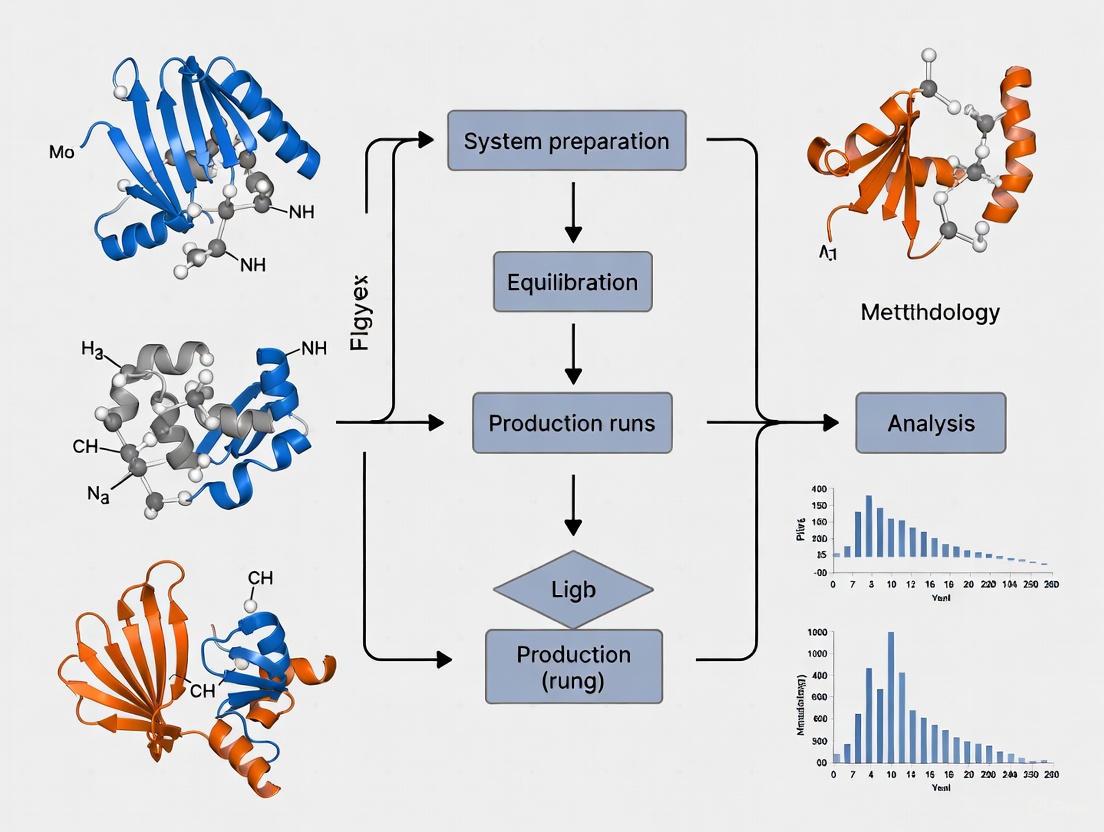
The following diagram illustrates the logical sequence of a standard molecular dynamics simulation protocol for a protein-ligand complex, integrating steps from the methodologies described above.

Standard MD Simulation Workflow

For advanced studies focusing on binding free energies, the dPaCS-MD/MSM method provides a specialized workflow, depicted below.

Enhanced Sampling for Binding Free Energy

Key Force Fields for Protein-Ligand Interactions (e.g., AMBER, CHARMM)

Molecular dynamics (MD) simulations have become an indispensable tool in structural biology and computer-aided drug design, providing atomic-level insight into protein-ligand interactions that is difficult to obtain through experimental methods alone. The accuracy of these simulations critically depends on the empirical force fields used to represent the potential energy surface of the molecular system. Force fields are mathematical representations of the potential energy of a system of particles, comprising parameters for bonded interactions (bonds, angles, dihedrals) and non-bonded interactions (van der Waals, electrostatics). For protein-ligand interactions, the choice of force field significantly impacts the reliability of binding mode predictions, binding affinity estimates, and conformational sampling. The most widely used force families for biomolecular simulations are AMBER (Assisted Model Building with Energy Refinement) and CHARMM (Chemistry at HARvard Macromolecular Mechanics), which have been continuously refined over decades to improve their accuracy for proteins, nucleic acids, lipids, carbohydrates, and small molecules. This application note provides a comprehensive overview of these key force fields, their performance characteristics, and detailed protocols for their application in studying protein-ligand interactions.

AMBER Force Field Family

The AMBER force field family includes several specialized parameter sets for biomolecules. The protein force fields, particularly AMBER ff14SB and ff19SB, are optimized for simulating proteins and are often combined with the General AMBER Force Field (GAFF and GAFF2) for small molecules. GAFF2 is specifically designed to provide atom types and parameters needed to parameterize most pharmaceutical molecules and maintains compatibility with traditional AMBER force fields for proteins [6]. For charge assignment, the AM1-BCC method provides an inexpensive and fast approach for calculating partial charges, which is particularly useful for high-throughput applications [6] [7].

The AMBER force field functional form includes terms for bonds, angles, dihedrals, and non-bonded interactions similar to CHARMM, though it does not include explicit Urey-Bradley terms for angle compensation [8]. In benchmark studies, AMBER ff14SB has demonstrated excellent performance in representing protein side chain ensembles, showing particularly high accuracy for buried residues compared to surface-exposed ones [9].

CHARMM Force Field Family

The CHARMM force fields encompass multiple generations of parameter sets for different biomolecular classes. CHARMM36 is the current standard for proteins, lipids, and nucleic acids, while CHARMM36m represents an improved version for proteins that better captures intrinsically disordered regions [10] [11]. For drug-like molecules, the CHARMM General Force Field (CGenFF) provides broad coverage of chemical groups present in biomolecules and pharmaceuticals [8] [10].

The CHARMM potential energy function includes distinctive terms not present in all force fields:

[ \begin{aligned} V = &\sum{bonds}k{b}(b-b{0})^{2} + \sum{angles}k{\theta}(\theta-\theta{0})^{2} + \sum{dihedrals}k{\phi}[1+\cos(n\phi-\delta)] \ &+ \sum{impropers}k{\omega}(\omega-\omega{0})^{2} + \sum{Urey-Bradley}k{u}(u-u{0})^{2} \ &+ \sum{nonbonded}\left(\epsilon{ij}\left[\left(\frac{R{min{ij}}}{r{ij}}\right)^{12}-2\left(\frac{R{min{ij}}}{r{ij}}\right)^{6}\right]+\frac{q{i}q{j}}{\epsilon{r}r{ij}}\right) \end{aligned} ]

The Urey-Bradley term specifically contributes to angle vibrations, while the improper term accounts for out-of-plane bending [8]. CHARMM also includes developing polarizable force fields using both the fluctuating charge (CHEQ) and Drude shell models to more accurately represent electronic polarization effects [10].

Comparative Performance in Protein-Ligand Studies

Recent benchmarking studies provide quantitative comparisons of force field performance for protein-ligand interactions. In side chain conformation studies, AMBER and CHARMM force fields clearly outperform OPLS and GROMOS in estimating rotamer populations, with AMBER14SB, AMBER99SB*-ILDN, and CHARMM36 identified as the best performers [9].

For binding free energy calculations, comprehensive assessments have evaluated various parameter combinations. The table below summarizes performance metrics for different force field and water model combinations in Free Energy Perturbation (FEP) calculations on eight benchmark test cases (BACE, CDK2, JNK1, MCL1, P38, PTP1B, Thrombin, TYK2) [7]:

Table 1: Force Field Performance in Binding Free Energy Prediction

Force Field	Water Model	Charge Model	Mean Unsigned Error (kcal/mol)	RMSE (kcal/mol)	R²
AMBER ff14SB	SPC/E	AM1-BCC	0.89	1.15	0.53
AMBER ff14SB	TIP3P	AM1-BCC	0.82	1.06	0.57
AMBER ff14SB	TIP4P-EW	AM1-BCC	0.85	1.11	0.56
AMBER ff15ipq	SPC/E	AM1-BCC	0.85	1.07	0.58
AMBER ff14SB	TIP3P	RESP	1.03	1.32	0.45
AMBER ff15ipq	TIP4P-EW	AM1-BCC	0.95	1.23	0.49
OPLS2.1 (FEP+)	-	-	0.77	0.93	0.66
AMBER (TI)	-	-	1.01	1.30	0.44

These results demonstrate that the combination of AMBER ff14SB with TIP3P water and AM1-BCC charges provides the best balance of accuracy among the open-source options tested, with performance approaching that of commercial implementations like OPLS2.1 used in Schrödinger's FEP+ [7].

Experimental Protocols and Workflows

Ligand Parameterization Protocol for AMBER/GAFF2

Accurate parameterization of small molecule ligands is essential for reliable MD simulations. The following protocol uses AmberTools programs to generate parameters for non-conventional residues [6]:

• Input Preparation: Prepare a 3D structure of the ligand in PDB or MOL2 format with correct protonation states and stereochemistry.

• Atom Typing and Charge Calculation:

  This command assigns GAFF2 atom types and calculates AM1-BCC partial charges for the neutral molecule[-] [6]. The -nc option specifies the net molecular charge, which should be adjusted according to the ligand's protonation state.

• Parameter Checking:

  This step identifies missing force field parameters and provides reasonable approximations by analogy to similar parameters [6]. The resulting frcmod file should be carefully inspected, particularly for any parameters marked with "ATTN: needs revision" which require manual parameterization.

• File Integration in tLEaP:

  These commands load the generated parameters into the AMBER simulation environment [12].

System Assembly and Simulation Setup

The workflow below illustrates the complete process for building and simulating a protein-ligand complex:

Diagram 1: MD Setup Workflow (65 characters)

For CHARMM simulations, the CHARMM-GUI platform provides a robust alternative for system building, offering automated parameter assignment through its Ligand Reader & Modeler module [10]. This web-based interface can generate input files for multiple simulation packages including CHARMM, NAMD, GROMACS, AMBER, and OpenMM.

Virtual Screening Enhancement Protocol

Molecular docking followed by MD refinement has emerged as a powerful approach for improving virtual screening results. The following protocol demonstrates this integrated methodology [11]:

• Initial Docking: Perform molecular docking with AutoDock Vina or similar software to generate initial protein-ligand poses.

• High-Throughput MD Setup:

  • Convert docked poses to MD-ready systems using automated tools like CHARMM-GUI's Input Generator.
  • Employ a python script to automate browser actions for batch system preparation.

• Short MD Simulations:

  • Solvate systems in a cubic TIP3P water box with 10 Ã… padding.
  • Neutralize with appropriate ions (K+, Cl-).
  • Use the CHARMM36m force field for proteins and CGenFF for ligands.
  • Minimize (5,000 steps), equilibrate (1 ns NVT), and run production simulations (10-50 ns).

• Trajectory Analysis:

  • Calculate ligand RMSD relative to the initial docked pose after aligning the protein.
  • Identify stable binding modes based on RMSD convergence.
  • Use binding stability to discriminate active from decoy compounds, significantly improving enrichment over docking alone [11].

This approach has demonstrated a 22% improvement in ROC AUC (from 0.68 to 0.83) compared to docking alone across 56 protein targets from the DUD-E dataset [11].

Research Reagent Solutions

Table 2: Essential Tools for Protein-Ligand MD Simulations

Tool/Resource	Type	Primary Function	Compatibility
AmberTools	Software Suite	Ligand parameterization with antechamber/parmchk2, system building with tLEaP	AMBER force fields
CHARMM-GUI	Web Portal	Automated system building for membrane and soluble proteins	CHARMM, AMBER, GROMACS, NAMD
CGenFF	Force Field	Parameterization of drug-like molecules	CHARMM force fields
GAFF/GAFF2	Force Field	Parameterization of pharmaceutical molecules	AMBER force fields
OpenMM	MD Engine	High-performance GPU-accelerated simulations	Multiple force fields
CHARMM	MD Engine	Comprehensive biomolecular simulation package	CHARMM force fields

Advanced Applications and Methodological Developments

Free Energy Perturbation for Binding Affinity Prediction

Free energy perturbation (FEP) calculations have become increasingly reliable for predicting relative binding affinities of congeneric ligands. The automated FEP workflow implemented in tools like Alchaware using OpenMM provides open-source access to this methodology [7]. Key considerations for FEP setup include:

• Force Field Selection: AMBER ff14SB with GAFF2 and TIP3P water provides a well-validated combination.
• Charge Model: AM1-BCC charges generally outperform RESP for relative binding free energy calculations [7].
• Enhanced Sampling: Hamiltonian replica exchange with solute tempering (REST) improves convergence by enhancing conformational sampling [7].

Validation on eight benchmark targets demonstrated mean unsigned errors of 0.82-0.89 kcal/mol for binding affinity prediction, approaching chemical accuracy [7].

Specialized Force Fields for Membrane Proteins

Simulating membrane protein-ligand interactions requires additional considerations for the lipid environment. The AMBER LIPID21 force field provides parameters for various lipid types that are compatible with the protein ff14SB and GAFF2 small molecule force fields [13]. For complex membrane systems containing glycolipids or glycoproteins, the GLYCAM_06j force field can be combined with AMBER parameters for comprehensive coverage [13].

Emerging Methodologies

Recent developments in force fields include the creation of residue-specific parameters for intrinsically disordered proteins (CHARMM36IDPSFF) which improve agreement with experimental NMR chemical shifts [10]. The continued refinement of polarizable force fields, particularly the CHARMM Drude model, promises more accurate representation of electronic effects in heterogeneous binding environments [10].

Integration of MD with experimental structural biology approaches has also shown promise, as demonstrated in studies where enrichment of chemical libraries docked to protein conformational ensembles from MD simulations led to successful identification of novel aldehyde dehydrogenase 2 inhibitors with IC50 values below 5 μM [14].

The accuracy of molecular dynamics (MD) simulations is fundamentally constrained by the quality of the initial structural models. Preparing and refining protein-ligand complexes represents a critical first step in any MD pipeline, as errors introduced at this stage propagate through subsequent analysis, compromising biological interpretations and drug discovery applications. Current research emphasizes that widely-used datasets often contain structural artifacts in both proteins and ligands, which undermine the accuracy and generalizability of resulting scoring functions and dynamic profiles [15]. This application note details standardized protocols for structure preparation, highlighting integrated computational workflows that transform raw coordinate data into simulation-ready systems, while providing metrics for quality assessment throughout the process.

Key Challenges in Initial Structure Preparation

Common Structural Artifacts and Data Issues

Protein-ligand complexes derived from experimental sources, particularly crystallography, frequently contain imperfections that necessitate correction before MD simulation. Analysis of popular datasets like PDBbind reveals several recurring issues that require systematic addressing [15]:

Table 1: Common Structural Artifacts in Protein-Ligand Complexes

Category	Specific Issues	Impact on Simulation
Ligand Issues	Incorrect bond orders, unrealistic protonation states, missing hydrogen atoms, improper aromaticity	Compromised electrostatic interactions, inaccurate binding energy calculations, distorted binding poses
Protein Issues	Missing heavy atoms in residues, unresolved loops, incorrect side chain rotamers, missing disulfide bridges	Altered protein flexibility, non-physical conformational sampling, distorted binding pocket geometry
Complex Issues	Severe steric clashes between protein and ligand, covalently bonded ligands misclassified as non-covalent, unrealistic binding orientations	Simulation instability, need for excessive equilibration, fundamentally incorrect binding mechanism
Data Organization	Sub-optimal organization of protein-ligand classes, inconsistent curation protocols	Limited training and validation capabilities for scoring functions

The presence of these artifacts underscores why a robust preparation workflow is indispensable. As one study notes, "a significant portion of the PDBbind dataset contains structural errors, statistical anomalies, and a sub-optimal organization of protein-ligand classes that can limit SF training and validation" [15].

Workflow for Structural Preparation and Refinement

A semi-automated workflow approach ensures reproducibility while minimizing manual intervention. The following diagram illustrates a comprehensive pipeline for converting raw structural data into simulation-ready systems:

Standardized Protocols for Structure Preparation

Integrated Protein-Ligand Preparation Workflow

Objective: Transform raw PDB structures into simulation-ready systems with corrected chemistry and complete atom representation.

Materials and Software Requirements:

• Input Data: Protein-ligand complex structure in PDB format
• Structure Preparation Tools: Chimera, Schrodinger Maestro, MOE, or similar
• Ligand Parameterization: LigParGen server, CGenFF, ACPYPE, AnteChamber
• Force Fields: OPLS-AA, CHARMM, AMBER, or GROMOS families
• MD Engines: GROMACS, AMBER, NAMD, or CHARMM

Step-by-Step Protocol:

• Structure Cleaning and Validation

  • Download PDB structure and separate protein, ligand, and additive components (ions, cofactors, solvents)
  • Remove alternative conformations, retaining only the highest occupancy atoms
  • Validate ligand geometry against chemical component dictionary
  • Check for structural completeness using visual inspection and validation servers

• Protein Structure Preparation

  • Add missing heavy atoms using loop modeling approaches (e.g., Dunbrack rotamer library)
  • Correct histidine protonation states based on local environment and predicted pKa values
  • Add disulfide bonds where appropriate based on cysteine proximity
  • Optimize side-chain rotamers for residues outside binding pocket

• Ligand Structure Preparation

  • Correct bond orders and aromaticity using chemical knowledge
  • Determine appropriate protonation states at physiological pH (considering local environment)
  • Perform geometry optimization with quantum mechanical methods or molecular mechanics
  • Generate topology files with appropriate charge models (e.g., 1.14*CM1A for neutral ligands)

• Complex Reassembly and Validation

  • Recombine corrected protein and ligand structures
  • Add missing hydrogen atoms to entire system
  • Perform constrained energy minimization to relieve steric clashes
  • Validate final structure against experimental electron density where available

Troubleshooting Tips:

• For ligands with unusual chemistry, consider manual parameterization using quantum mechanical approaches
• If severe clashes persist after minimization, consider alternative ligand binding poses
• For membrane proteins, include membrane environment during preparation stages

Practical Application: GROMACS Protein-Ligand System Setup

Case Study: T4 Lysozyme L99A with Benzene (PDB ID: 4W52)

This protocol provides a specific implementation for GROMACS simulations [16]:

• Structure Preparation

  This produces protein_clean.pdb and ligand_wH.pdb

• Ligand Parameterization

  • Upload ligand_wH.pdb to LigParGen server with residue number set to 1
  • Select appropriate charge model (1.14*CM1A for neutral ligands)
  • Download GROMACS files: BNZ.gro (coordinates) and BNZ.itp (topology)

• System Assembly

• Topology Integration

  • Add #include "BNZ.itp" to topol.top after forcefield inclusion
  • Add BNZ 1 to [molecules] section

The resulting system is then ready for solvation, ionization, and energy minimization according to standard MD protocols [16].

Quality Assessment and Validation Metrics

Validation Framework for Prepared Structures

Quality validation should employ multiple complementary metrics to assess different aspects of structural integrity. The Metrics Reloaded framework provides a paradigm for multi-dimensional assessment, recommending against reliance on single metrics [17].

Table 2: Quality Metrics for Prepared Protein-Ligand Structures

Metric Category	Specific Metrics	Optimal Range	Assessment Method
Steric Quality	Clash score, Ramachandran outliers, Rotamer outliers	Clash score < 10, Ramachandran favored > 95%	MolProbity, WHAT_CHECK
Geometry Quality	Bond length deviations, Bond angle deviations, RMSZ scores	RMSZ < 1.0 for bonds and angles	REFMAC, Phenix validation
Ligand Chemistry	Planarity violations, Chirality errors, Bond length outliers	No violations	Privateer, Grade Web Server
Electronic Properties	Partial charge rationality, Dipole moment consistency	Comparable to QM calculations	Quantum mechanical calculations
Complex Compatibility	Complementarity statistics, Interface voids	Sc > 0.60, minimal voids	SC, PISA, 3D-surfer

The importance of multi-metric validation is emphasized by recent research: "By definition, each metric comes with specific, task-dependent pitfalls. An overlap-based metric... is not able to capture the object shape properly. On the other hand, a boundary-based metric... may miss holes inside an object. Both metrics combined would complement each other" [17].

Advanced Refinement Techniques

For challenging cases where standard preparation yields unsatisfactory results, advanced refinement techniques can be employed:

Ensemble Refinement: This method accounts for ligand flexibility in crystal structures by generating multiple conformations, providing insights beyond standard refinement. Research shows that "ensemble refinement sometimes indicates that the flexibility of parts of the ligand and some protein side chains is larger than that which can be described by a single conformation" [18].

Molecular Dynamics with Enhanced Sampling: Short simulations with accelerated sampling (e.g., Gaussian accelerated MD, metadynamics) can explore alternative binding modes and identify the most stable conformation before production runs.

QM/MM Refinement: For critical ligand interactions, quantum mechanical/molecular mechanical optimization of the binding site provides superior electronic structure description compared to force field methods alone.

Research Reagent Solutions

Table 3: Essential Tools for Protein-Ligand Structure Preparation

Tool Name	Type	Primary Function	Access
LigParGen	Web Server	OPLS-AA parameter generation for organic ligands	https://ligpargen.scs.illinois.edu
HiQBind-WF	Workflow	Data cleaning and structural preparation pipeline	Open-source [15]
Chimera	Desktop Software	Structure visualization, analysis, and initial preparation	https://www.cgl.ucsf.edu/chimera
PDB2GMX	GROMACS Tool	Protein topology generation with hydrogens	Part of GROMACS suite
BioLiP	Database	Protein-ligand interactions with functional annotations	https://bindingdb.org/bind/BioLiP3
MolProbity	Web Service	All-atom structure validation	http://molprobity.biochem.duke.edu
Grade	Web Server	Ligand geometry evaluation and idealization	https://grade.globalphasing.org

Proper preparation of initial protein-ligand structures remains a non-negotiable prerequisite for reliable molecular dynamics simulations. By implementing the standardized protocols and validation metrics outlined in this application note, researchers can significantly enhance the accuracy and interpretability of their simulation results. The integration of automated workflows like HiQBind-WF with careful manual inspection represents the current state-of-the-art approach, balancing efficiency with rigorous quality control. As MD simulations continue to play an increasingly central role in drug discovery and structural biology, robust preparation methodologies will only grow in importance for generating biologically meaningful insights.

The accuracy of molecular dynamics (MD) simulations of protein-ligand complexes is critically dependent on the faithful representation of the simulation environment. Solvation, ion concentration, and system neutralization are not merely procedural steps but foundational aspects that govern the electrostatic and steric interactions central to biomolecular function and ligand binding [19]. An improperly solvated system or an imbalanced ionic atmosphere can lead to simulation artifacts, unreliable trajectories, and ultimately, incorrect biological inferences. The environment must be modeled to mimic the physiological conditions relevant to the system under study, whether for fundamental research or computer-aided drug discovery. This document outlines the core concepts, quantitative parameters, and detailed protocols for defining a physiologically realistic simulation environment, framed within the broader methodology for MD simulations of protein-ligand complexes.

Core Concepts and Solvation Models

The first and most significant choice in defining the environment is how to represent the solvent, which is typically water in biological systems. Solvation models fall into two primary categories: explicit and implicit, each with distinct advantages and computational trade-offs [20].

Explicit Solvent Models

Explicit solvent models treat solvent molecules as individual, discrete entities with defined coordinates and degrees of freedom. This approach provides a physically intuitive and spatially resolved picture of the solvent, allowing for the specific study of water structure, hydrogen-bonding networks, and solvent-mediated interactions.

• Physical Realism: Explicit models can capture specific solute-solvent interactions, such as water bridges between a protein and a ligand, which can be critical for accurate binding affinity predictions [21].
• Common Water Models: The TIP3P water model is a standard choice in many MD suites and is often a component of broader force fields like AMBER [2]. Other models, such as SPC (Simple Point Charge), are also widely used [20].
• Computational Cost: The primary disadvantage is computational expense, as the solvent molecules can constitute over 80% of the particles in a system, drastically increasing the computational resources required for the simulation.

Implicit Solvent Models

Implicit solvent models, also known as continuum models, replace explicit solvent molecules with a homogeneously polarizable medium characterized primarily by its dielectric constant (ε) [20]. The solute is embedded in a cavity within this continuum, and the model calculates the free energy of solvation based on the solute's charge distribution.

The solvation free energy (ΔG_solv) in these models is typically decomposed into several components [20]: ΔG_solv = G_cavity + G_{electrostatic} + G_dispersion + G_repulsion

Where:

• G_cavity: Energy required to create a cavity in the solvent for the solute.
• G_{electrostatic}: Energy from polarization of the solvent by the solute's charge distribution.
• G_dispersion and G_repulsion: Non-electrostatic contributions from van der Wa forces and exchange repulsion.

Popular implicit models include the Polarizable Continuum Model (PCM), the Solvation Model based on Density (SMD), and the COSMO (COnductor-like Screening MOdel) model [20] [22] [23]. The SMD model, for instance, is a "universal" model applicable to any solute in any solvent for which key descriptors like the dielectric constant and surface tension are known [23].

Table 1: Comparison of Common Implicit Solvation Models.

Model	Theoretical Basis	Key Features	Common Use Cases
PCM [20]	Poisson(-Boltzmann) Equation	Solute in a tiled cavity within a dielectric continuum; highly configurable.	Geometry optimizations, frequency calculations in solution.
SMD [23]	IEF-PCM / Universal	Uses full solute electron density; parametrized for a wide range of solvents and solutes.	Hydration free energy predictions, quantum chemical calculations.
COSMO [22]	Conductor-like Screening	Fast, robust approximation to dielectric equations; reduces outlying charge errors.	Self-consistent reaction field calculations in quantum chemistry.

Hybrid and Advanced Models

For specific applications, hybrid approaches are available. QM/MM (Quantum Mechanics/Molecular Mechanics) methods allow a section of the system (e.g., a ligand in a binding site) to be treated with quantum mechanical accuracy, while the rest of the protein and solvent is handled with a classical MM force field [20] [19]. Furthermore, a new generation of polarizable force fields, such as the AMOEBA (Atomic Multipole Optimised Energetics for Biomolecular Applications) force field, is being developed to account for changes in molecular charge distribution, providing a more accurate representation of electrostatic interactions in explicit solvent simulations [20].

Ion Concentration and System Neutralization

In a physiological environment, proteins and ligands exist in a solution containing ions. Omitting ions from a simulation can lead to severe electrostatic artifacts, especially when the protein-ligand complex carries a net charge.

Purpose of Ions in MD Simulations

• Charge Neutralization: The primary role of ions is to neutralize the net charge of the system. Most MD simulation codes, including GROMACS, require the total system charge to be zero to avoid infinite electrostatic self-energies in periodic boundary conditions. This is achieved by adding counter-ions (e.g., Na⁺ for a negatively charged system, Cl⁻ for a positively charged one) [24].
• Physiological Ionic Strength: Beyond neutralization, ions are added to achieve a specific physiological concentration (e.g., 150 mM NaCl). This creates an ionic atmosphere that screens electrostatic interactions, mirroring real biological conditions and improving the realism of the simulation [2] [25].

Practical Implementation

The process typically involves two steps:

• Neutralization: Adding the minimal number of counter-ions to bring the total system charge to zero.
• Salting: Adding additional pairs of cations and anions to reach a desired ionic concentration (e.g., 0.15 M for physiological saline) [25].

The ion concentration is usually specified in molar (M) units. The number of ions to add is calculated automatically by the MD software based on the volume of the simulation box and the number of water molecules present [25].

Table 2: Common Ion Types and Parameters in MD Simulations.

Ion Type	Force Field Parameters	Common Concentration	Purpose
Na⁺	Included in major force fields (CHARMM36, AMBER)	0.15 M [2]	Physiological salt concentration (as NaCl)
K⁺	Included in major force fields (CHARMM36, AMBER)	0.15 M [25]	Physiological salt concentration (as KCl); often used as default [25]
Cl⁻	Included in major force fields (CHARMM36, AMBER)	0.15 M [2]	Counter-ion for positive systems; physiological salt

Experimental Protocols and Workflows

This section provides a detailed, step-by-step protocol for setting up a simulation environment for a protein-ligand complex, leveraging tools like GROMACS and OpenFE [24] [2].

Comprehensive Setup Workflow

The following diagram outlines the complete workflow for defining the simulation environment, from initial structure preparation to a production-ready system.

Detailed Protocol for System Setup

The following steps provide a command-line-centric protocol using GROMACS, a widely used MD software package [24].

Step 1: Obtain and Prepare Protein and Ligand Coordinates

• Input: A protein structure file in PDB format. If the structure contains a ligand of interest, its coordinates must be present.
• Action: Visually inspect the structure using a molecular viewer (e.g., RasMol). Pre-process the PDB file to remove extraneous water molecules and other non-essential components. For ligands not recognized by the force field, separate topology files must be created manually [24].
• Command (GROMACS):
  This command generates the molecular topology and coordinate file in GROMACS format, prompting the user to select an appropriate force field.

Step 2: Define the Simulation Box and Apply Periodic Boundary Conditions

• Purpose: To create a finite simulation cell that can be replicated infinitely in space, thus avoiding artificial surface effects.
• Action: Define a box (e.g., cubic, dodecahedron) around the protein with a sufficient margin (e.g., 1.4 nm) from the protein surface to ensure the solute does not interact with its own periodic images [24].
• Command (GROMACS):

Step 3: Solvate the System

• Purpose: To immerse the protein-ligand complex in a solvent environment.
• Action: Fill the simulation box with water molecules. This updates the topology file to include the water molecules.
• Command (GROMACS):

• Alternative (OpenFE): In modern workflows using tools like OpenFE, the SolventComponent is defined with parameters for the solvent model (e.g., tip3p) and solvent padding (e.g., 1.0 nm), which automates this step [2].

Step 4: Add Ions for Neutralization and Physiological Concentration

• Purpose: To neutralize the system's net charge and establish a physiologically relevant ionic strength.
• Prerequisite: Generate a pre-processed input file (*.tpr) using the grompp command and a parameter file (*.mdp).
• Action: Use the genion command to replace water molecules with ions.
• Command (GROMACS):
  This example adds 3 chloride ions (CL) to neutralize a system with a net charge of -3. The -pname and -nname flags specify the cation and anion types, respectively [24].
• Alternative (OpenFE): The SolventComponent can be initialized with an ion_concentration parameter (e.g., 0.15 * unit.molar) and an ions_type (e.g., KCl or NaCl), which handles this process during system setup [2] [25].

The Scientist's Toolkit: Essential Research Reagents and Software

The following table catalogs key software tools and "reagents" essential for setting up a simulation environment for protein-ligand complexes.

Table 3: Essential Software and Parameters for Simulation Environment Setup.

Item Name	Type / Category	Function in Setup Process	Example Parameters / Notes
GROMACS [24]	MD Software Suite	Performs all steps: file conversion, solvation, ion addition, minimization, equilibration, and production MD.	Open-source; high performance; supports major force fields.
OpenFE/OpenMM [2]	MD Automation & Engine	Python-based toolkit for setting up and running simulation workflows, including complex protein-ligand systems.	Simplifies setup via ChemicalSystem and settings objects; uses OpenMM as a backend.
CHARMM36 [25]	Force Field	Provides molecular mechanics parameters for proteins, lipids, nucleic acids, and small molecules.	Commonly used with GROMACS; includes TIP3P water model parameters.
AMBER ff14SB [2]	Force Field	Provides molecular mechanics parameters for proteins. Often used with TIP3P water.	Default in some OpenFE protocols [2].
TIP3P [2]	Explicit Water Model	A 3-site model for water molecules. Used to solvate the system explicitly.	Standard choice for simulations with AMBER and CHARMM force fields.
SMD Model [23]	Implicit Solvent Model	A universal solvation model for calculating solvation free energies in quantum chemical calculations.	Uses solute electron density; parametrized for a wide range of solvents.
Na+/K+/Cl- [25]	Ion Parameters	Pre-defined parameters within force fields for adding ions for neutralization and physiological concentration.	ions_type=NaCl or ions_type=KCl; ions_conc=0.15 (for 0.15 M) [25].
Yrgds	Yrgds, MF:C24H36N8O10, MW:596.6 g/mol	Chemical Reagent	Bench Chemicals
Dmbap	Dmbap, MF:C19H28N2O5, MW:364.4 g/mol	Chemical Reagent	Bench Chemicals

The careful definition of the simulation environment is a critical, non-negotiable step in generating reliable and meaningful MD simulations of protein-ligand complexes. The choice between explicit and implicit solvation involves a strategic trade-off between computational cost and the level of physical detail required. The subsequent steps of system neutralization and the establishment of a physiological ion concentration are essential for creating a stable, electrostatically realistic system. By adhering to the detailed protocols and utilizing the tools outlined in this document, researchers can ensure that their simulations are built upon a solid foundation, thereby increasing the credibility of their scientific findings in the broader context of drug development and biomolecular research.

Energy Minimization and Equilibration Protocols for Stable Starting Points

Within the broader methodology for molecular dynamics (MD) simulations of protein-ligand complexes, the establishment of a stable and physically realistic starting point is a critical prerequisite for obtaining reliable results. Energy minimization and equilibration protocols serve as the foundational steps that transition a system from its initial, potentially strained coordinates to a stable, equilibrium state representative of the biological conditions under investigation. Without proper minimization and equilibration, simulations can exhibit unrealistic atomic clashes, high-energy conformations, and unstable trajectories that compromise the validity of subsequent production runs and binding free energy calculations [5] [26]. This application note details comprehensive protocols for preparing stable systems, drawing from established methodologies in the field [2] [27] [28].

The necessity of these steps stems from several inherent issues in initial protein-ligand complex structures. These may include steric clashes introduced during docking or homology modeling, deviations from ideal bond geometries, and the abrupt introduction of solvent molecules and counterions into the system [29] [27]. Energy minimization gradually relieves these steric strains and geometric distortions by iteratively adjusting atomic coordinates to find a local minimum on the potential energy surface. Subsequent equilibration then allows the system to adopt appropriate thermodynamic properties—including correct temperature, density, and pressure—through carefully controlled dynamics that prevent the collapse of the protein structure or premature dissociation of the ligand [2] [28].

Theoretical Framework

The Role of Energy Minimization

Energy minimization in molecular dynamics functions as a corrective process that resolves structural imperfections in the initial molecular system. By employing algorithms such as steepest descent, conjugate gradient, or limited-memory Broyden–Fletcher–Goldfarb–Shanno (L-BFGS), minimization progressively reduces the total potential energy of the system until a convergence threshold is met [29]. This process is essential for removing unphysical atomic overlaps that would otherwise create enormous forces and numerical instabilities if directly subjected to dynamics.

The mathematical foundation of minimization relies on the calculation of the potential energy function, typically represented by a molecular mechanics force field:

[ E{\text{total}} = E{\text{bond}} + E{\text{angle}} + E{\text{torsion}} + E{\text{electrostatic}} + E{\text{van der Waals}} ]

where the various terms represent bond stretching, angle bending, torsional rotations, electrostatic interactions, and van der Waals forces, respectively [26]. Minimization algorithms iteratively adjust atomic coordinates to locate minima on this multidimensional energy surface, ensuring the system begins dynamics from a stable configuration.

Equilibration Principles

Equilibration bridges the gap between a statically minimized structure and a system ready for production MD under the desired thermodynamic ensemble. This phase allows for the gradual relaxation of solvent molecules around the solute, proper distribution of kinetic energy among all degrees of freedom, and establishment of correct system density and temperature [2] [28]. A well-designed equilibration protocol typically follows a sequential approach:

• Position-restrained equilibration: Initially, heavy atoms of the protein and ligand are harmonically restrained while allowing solvent and ions to move freely. This enables water and ions to reorganize around the solute without destabilizing the protein-ligand complex.
• Gradual heating: The system temperature is progressively increased from a low value (e.g., 0-100K) to the target temperature (e.g., 300K) while maintaining restraints on solute heavy atoms.
• Pressure equilibration: Once the target temperature is reached, pressure coupling is introduced to achieve the correct system density, typically using a barostat for the NPT (constant Number of particles, Pressure, and Temperature) ensemble.

This staged approach prevents the "shocking" of the system with full dynamics immediately after minimization, which could lead to unrealistic structural deformations or ligand dissociation [28].

Computational Toolkit

Successful implementation of minimization and equilibration protocols requires specific computational tools and resources. The selection of software, force fields, and hardware configurations significantly impacts the efficiency and reliability of the preparatory stages.

Table 1: Essential Software Tools for Minimization and Equilibration

Software	Version	Primary Function	Application in Protocol
GROMACS	2023.4 [27]	Molecular dynamics simulation engine	Performing energy minimization, heating, equilibration, and production MD
AMBER	14+ [28]	Molecular dynamics suite	System preparation, parameterization, and initial minimization
OpenMM	7.6+ [2]	High-performance MD toolkit	Customizable MD protocols with GPU acceleration
AutoDock Tools	4.2 [27]	Docking and preparation software	Ligand preparation and parameterization
PyMOL	2.5 [27]	Molecular visualization	Structure analysis and validation
VMD	1.9.4 [27]	Visualization and analysis	Trajectory analysis and structure quality checks
MODELLER	10.7 [27]	Homology modeling	Protein structure completion for missing residues
CoPoP	CoPoP Liposome|Cobalt Porphyrin-Phospholipid|RUO	CoPoP (Cobalt Porphyrin-Phospholipid) for his-tagged antigen display in vaccine research. This product is For Research Use Only (RUO). Not for human or veterinary diagnostic use.	Bench Chemicals
bPiDI	bPiDI, MF:C22H34I2N2, MW:580.3 g/mol	Chemical Reagent	Bench Chemicals

Table 2: Recommended Hardware Configurations

Component	High-Performance Workstation	Standard Research Computer
Processor	Intel Core i9-14900K × 32 [27]	AMD Ryzen 5 5600x 6-core [27]
Memory	32 GB RAM [27]	32 GB RAM [27]
GPU	NVIDIA GeForce RTX 4080 [27]	NVIDIA GeForce RTX 3060 [27]
Storage	5.9 TB [27]	2.5 TB [27]
Operating System	Ubuntu 22.04.5 LTS [27]	Ubuntu 22.04.3 LTS [27]

Specialized force fields provide the fundamental parameters governing atomic interactions during minimization and equilibration. For protein-ligand systems, recommended force fields include:

• AMBER ff14SB [2]: For protein parameters, offering improved side chain torsions and backbone adjustments.
• OpenFF-2.2.1 [2]: For small molecule force fields, providing accurate ligand parameterization.
• TIP3P [2]: For water models, balanced between computational efficiency and accuracy.

Additional specialized force fields like CHARMM36 and GAFF may be selected based on specific system requirements and research group experience [27] [26].

Core Methodological Framework

The following section outlines a comprehensive, step-by-step protocol for energy minimization and equilibration of protein-ligand complexes, synthesizing best practices from established methodologies [2] [27] [28].

Figure 1: Complete workflow for energy minimization and equilibration of protein-ligand complexes, showing the sequential steps from initial structure to stable system ready for production MD.

System Preparation and Parameterization

A. Initial Structure Preparation

Begin with a high-resolution structure of the protein-ligand complex, preferably from crystallography or cryo-EM. For modeled complexes, ensure the binding pose is validated through docking scores and interaction analysis [27] [28].

• Structure Processing:

  • Remove crystallographic water molecules except those forming critical bridging interactions with the ligand (typically within 5Ã…) [28].
  • Add missing hydrogen atoms using tools like PyMOL or CHARMM-GUI, adjusting protonation states to match physiological pH (e.g., GLU, ASP deprotonated; LYS, ARG protonated) [27].
  • For histidine residues, determine the appropriate protonation state (HID, HIE, or HIP) based on the local hydrogen bonding environment.

• Ligand Parameterization:

  • Generate ligand parameters using appropriate tools:

  • Assign partial charges using AM1-BCC [2] or higher-level quantum mechanical methods for critical interactions.

B. Solvation and Ion Placement

• Solvation:

  • Place the complex in an appropriate water box (e.g., dodecahedral or rectangular) with a minimum solvent padding of 1.0 nm between the protein and box edges [2].
  • Use compatible water models such as TIP3P [2] or SPC/E depending on the chosen force field.

• Ion Addition:

  • Add ions to neutralize the system net charge, followed by additional ions to achieve physiological concentration (e.g., 0.15 M NaCl) [2] [27].
  • Replace solvent molecules with ions using automated tools like tleap in AMBER or gmx genion in GROMACS.

Staged Energy Minimization Protocol

A multi-stage minimization approach gradually relaxes the system while maintaining structural integrity [27] [28]. The following protocol employs sequentially decreasing restraint weights:

Table 3: Staged Energy Minimization Parameters

Stage	Restraints Applied	Force Constant	Algorithm	Convergence Criteria
1. Heavy Restraint	All protein and ligand heavy atoms	500 kcal/mol/Ų [28]	Steepest Descent	Maximum force < 1000 kJ/mol/nm
2. Backbone Restraint	Protein backbone atoms only	50 kcal/mol/Ų [28]	Conjugate Gradient	Maximum force < 500 kJ/mol/nm
3. Full System	No restraints	Not applicable	L-BFGS	Maximum force < 100 kJ/mol/nm

Implementation Notes:

• Stage 1: This strong restraint stage relieves severe steric clashes while maintaining the overall protein-ligand structure.
• Stage 2: With reduced restraints on side chains, this allows side chain rearrangements and relief of localized strains.
• Stage 3: The final stage allows the entire system to relax to a local energy minimum without constraints.

Monitor convergence through the evolution of the potential energy and the maximum force. The minimization should proceed until the energy change between steps becomes negligible and forces fall below the specified thresholds.

System Equilibration Procedure

Following minimization, the system requires careful equilibration to reach the target thermodynamic state. The protocol below describes a multi-stage approach:

Table 4: Detailed Equilibration Protocol Parameters

Stage	Ensemble	Restraints	Temperature	Duration	Thermostat/Barostat
Heating	NVT	Protein and ligand heavy atoms (force: 50 kcal/mol/Ų) [28]	0K → 100K → 200K → 300K	50-100 ps per step	Langevin (collision frequency: 1 ps⁻¹) [2]
Density Equilibration	NPT	Protein and ligand heavy atoms (force: 10 kcal/mol/Ų) [28]	300K	100-200 ps	Berendsen [28] → Parrinello-Rahman [2]
Unrestrained Equilibration	NPT	None	300K	500 ps - 1 ns	Nosé-Hoover [2]

Critical Steps:

• Heating Phase:

  • Gradually increase system temperature in steps while maintaining strong positional restraints on protein and ligand heavy atoms.
  • Use a Langevin thermostat with a collision frequency of 1.0 ps⁻¹ for efficient temperature coupling [2].

• Density Equilibration:

  • Switch to NPT ensemble with moderate positional restraints (10 kcal/mol/Ų) on solute heavy atoms.
  • Use semi-isotropic pressure coupling for membrane systems or isotropic for soluble proteins.
  • Initially use Berendsen barostat for rapid equilibration, then switch to Parrinello-Rahman for production dynamics [2].

• Unrestrained Equilibration:

  • Remove all positional restraints for final equilibration.
  • Monitor system stability through potential energy, temperature, pressure, density, and root-mean-square deviation (RMSD) of protein backbone and ligand heavy atoms.

Validation and Quality Assessment

Before proceeding to production MD, validate the equilibrated system through multiple checks to ensure stability and proper equilibration.

A. Stability Metrics

• Energy Stability: The total potential energy should fluctuate steadily around a stable average without drifts.
• Temperature and Pressure: These should oscillate around the target values (300K, 1 bar) with reasonable fluctuations.
• Density: For aqueous systems, the density should converge to approximately 1000 kg/m³ for TIP3P water models.

B. Structural Integrity

• RMSD Analysis: Calculate the backbone RMSD relative to the minimized structure. The system is considered equilibrated when RMSD plateaus, typically within 1-3 Ã… for most globular proteins.
• Ligand Pose Stability: Monitor ligand RMSD to ensure it remains bound in the initial binding mode with minimal deviation.
• Secondary Structure Preservation: Verify that α-helices and β-sheets maintain their proper geometry through tools like DSSP.

C. Equilibration Duration Determination

The required equilibration time varies by system size and complexity. Use the following criteria to determine sufficient equilibration:

• Potential energy, temperature, and pressure show stable fluctuations around their averages.
• System density has stabilized to the expected value for the water model and conditions.
• Protein backbone RMSD has reached a plateau phase.

For typical protein-ligand systems (20,000-50,000 atoms), complete equilibration generally requires 1-5 ns total simulation time across all stages [2] [28].

Advanced Applications and Considerations

Membrane Protein Systems

For membrane-embedded proteins such as GABA (A) receptors [27], additional considerations apply:

• Membrane Embedding: Use tools like CHARMM-GUI to properly orient and embed the protein in a lipid bilayer (e.g., POPC membrane).
• Extended Minimization: Implement additional minimization steps with strong restraints on lipid headgroups to prevent membrane deformation.
• Staged Membrane Equilibration: Equilibrate the membrane with progressively decreasing restraints on lipid molecules while maintaining protein restraints.

Enhanced Sampling Preparations

When preparing systems for advanced sampling techniques like umbrella sampling or free energy perturbation:

• Extended Equilibration: Run longer equilibration phases (5-10 ns) to ensure thorough sampling of the bound state.
• Multiple Replicas: Generate multiple independent equilibration trajectories from different initial velocities to confirm convergence.
• Collective Variable Stability: Monitor proposed collective variables during equilibration to ensure they adequately describe the system dynamics.

Robust energy minimization and equilibration protocols provide the essential foundation for reliable molecular dynamics simulations of protein-ligand complexes. The staged approach outlined here—progressing from strongly restrained minimization through gradual heating and finally to unrestrained equilibration—ensures system stability while maintaining structural integrity. Through careful parameter selection, systematic execution, and rigorous validation, researchers can establish physically realistic starting points for subsequent production simulations and binding free energy calculations. This methodological framework supports accurate investigation of protein-ligand interactions across diverse biological systems, from soluble enzymes to membrane-bound receptors, advancing both fundamental understanding and drug discovery efforts.

Advanced Simulation Protocols and Analysis for Binding Kinetics and Energetics

Molecular dynamics (MD) simulations have become an indispensable tool in structural biology and drug discovery, providing atomic-level insights into the behavior of biomolecular systems over time. For the study of protein-ligand complexes, MD simulations offer a dynamic perspective that static crystal structures cannot, revealing conformational changes, binding pathways, and residence times critical for understanding drug action [30]. The configuration of production simulations—particularly the careful selection of timescales and parameters—represents a pivotal phase that directly determines the reliability and biological relevance of the simulation outcomes. Properly configured production runs can capture functionally relevant motions, quantify binding energetics, and provide insights into mechanisms of action, thereby bridging the gap between structural data and biological function [31] [32].

This protocol outlines a comprehensive methodology for configuring and executing production-level MD simulations of protein-ligand complexes, with emphasis on parameter selection, timescale considerations, and validation metrics appropriate for drug discovery research.

Fundamental Concepts and Simulation Timescales

Timescales of Biomolecular Processes

Different biological processes occur across vastly different timescales, which must be matched with appropriate simulation durations to obtain statistically meaningful results [30] [32]. The table below summarizes key protein-ligand dynamic events and their characteristic timescales:

Table 1: Characteristic Timescales for Protein-Ligand Dynamic Processes

Dynamic Process	Typical Timescale	Simulation Relevance
Side chain rotations	Picoseconds (10⁻¹² s) to nanoseconds (10⁻⁹ s)	Local flexibility, minor binding site adjustments
Loop motions	Nanoseconds to microseconds (10⁻⁶ s)	Gating of binding sites, accessible conformations
Ligand binding/unbinding	Microseconds to seconds	Residence time, binding affinity, drug efficacy
Large domain movements	Microseconds to milliseconds (10⁻³ s)	Allosteric regulation, major conformational changes
Protein folding	Milliseconds to seconds	Not typically addressed in ligand-binding studies

Evolution of Accessible Simulation Times

The trajectory of MD simulation capabilities shows exponential growth in accessible timescales:

Table 2: Historical Progression of MD Simulation Capabilities

Time Period	Typical Simulation Duration	System Size	Notable Achievements
1970s	Picoseconds (10⁻¹² s)	~500 atoms	First protein simulation (BPTI, 9.2 ps) [32]
1990s	Nanoseconds (10⁻⁹ s)	~10,000 atoms	Protein folding simulations, solvation studies
2000s	Tens to hundreds of nanoseconds	~100,000 atoms	Membrane protein simulations, ligand binding
2010s	Microseconds (10⁻⁶ s) to milliseconds	Millions of atoms	GPCR activation, protein folding, viral capsids
Present (2020s)	Milliseconds and beyond	Hundreds of millions of atoms	Entire organelles, gene simulation (1 billion atoms) [30]

Modern research demonstrates that long-timescale simulations (hundreds of microseconds) can reveal critical functional insights. For example, simulations aggregating 400-500 μs revealed how different protein kinase C activators (bryostatin, phorbol esters) differentially position the complex in membranes—a finding with profound implications for drug design [31].

System Configuration and Parameterization

Force Field Selection

The choice of force field constitutes a fundamental parameter that determines the accuracy of your simulation. Force fields provide the mathematical functions and parameters that describe the potential energy of a molecular system [33] [32].

Table 3: Comparison of Common All-Atom Force Fields for Protein-Ligand Simulations

Force Field	Proteins	Lipids	Nucleic Acids	Small Molecules	Key Features
CHARMM	CHARMM36m	CHARMM36	CHARMM36	CGenFF	Optimized for membrane systems; accurate lipid/protein interactions [32]
AMBER	ff19SB/ff14SB	LIPID21	OL15/OL3	GAFF	Balanced accuracy for proteins & nucleic acids; widely used [34] [32]
OPLS-AA	OPLS-AA/M	OPLS/L	-	-	Optimized for thermodynamic properties; good for peptides [32]
GROMOS	54A8	54A8	54A8	-	United-atom approach; faster calculations [32]

Simulation Parameters and Their Physical Significance

Production simulations require numerous parameters that collectively define the thermodynamic state and numerical integration scheme:

Integration Algorithms

• Velocity Verlet: Most common; numerically stable; good energy conservation
• Leap-frog: Computationally efficient; slightly less accurate [30]
• Time step: Typically 2 fs for all-atom simulations with constrained bonds involving hydrogens [34]

Thermodynamic Ensembles

• NPT (constant Number of particles, Pressure, Temperature): Most common for biomolecular simulations; mimics experimental conditions
• NVT (constant Number, Volume, Temperature): Useful for specific properties; less common for production
• Temperature coupling: Langevin thermostat or Nosé-Hoover chains maintain constant temperature [34]
• Pressure coupling: Parrinello-Rahman or Berendsen barostat maintain constant pressure (1 atm) [32]

Long-Range Electrostatics

• Particle Mesh Ewald (PME): Gold standard; accounts for long-range electrostatic interactions in periodic systems
• Cut-off methods: Less accurate but computationally cheaper; not recommended for production simulations [30]

Production Simulation Protocol

Pre-Production System Validation

Before initiating production simulations, thorough system validation is essential:

• Energy Minimization: 500-5000 steps of steepest descent or conjugate gradient to remove bad contacts [34]
• Equilibration Protocol:
  • Stage 1: 100 ps NVT simulation with positional restraints on protein and ligand (5 kcal mol⁻¹ Å⁻²)
  • Stage 2: 500 ps NPT simulation with restraints on ligand and protein backbone only [34]
• Equilibration Validation:
  • Stable potential energy (drift < 1-2%)
  • Protein backbone RMSD plateau (< 1.5-2 Ã… from starting structure)
  • Proper density convergence (~1 g/cm³ for aqueous systems)

Production Run Configuration

The production phase involves parameter choices that balance computational cost with scientific rigor:

Duration Guidelines

• Minimal sampling: 100 ns per system for initial assessment
• Adequate sampling: 500 ns - 1 μs for most protein-ligand conformational changes
• Comprehensive sampling: >1 μs for large-scale motions, binding/unbinding events [31]

System Sizing and Boundary Conditions

• Periodic Boundary Conditions: Standard approach to minimize edge effects
• Water padding: Minimum 10-15 Ã… between protein and box edge
• System size: Typically 50,000-200,000 atoms for a solvated protein-ligand complex [30]

Data Collection Parameters

• Trajectory saving frequency: Every 10-100 ps (balances resolution with storage)
• Energy data: Every 1-10 ps for thermodynamic analyses
• Checkpoint files: Frequent saves (every 1-5 ns) for simulation restart capability

Workflow for production MD simulations of protein-ligand complexes

The Scientist's Toolkit: Essential Research Reagents

Table 4: Essential Software and Tools for Production MD Simulations

Tool Category	Specific Software	Primary Function	Application Notes
Simulation Engines	GROMACS [30] [32]	High-performance MD simulation	Excellent parallelization; widely used in academia
	AMBER [30] [32]	MD simulation and analysis	Comprehensive toolset; strong force field development
	NAMD [30] [32]	Scalable MD simulations	Excellent for large systems; familiar interface
System Preparation	CHARMM-GUI [32]	Membrane system building	Streamlines complex system setup
	PACKMOL [34]	Initial system configuration	Solvation and ion placement
Force Fields	CGenFF/GAFF [32]	Small molecule parameters	Ligand parameterization for drug-like molecules
Analysis Tools	VMD [34] [32]	Trajectory visualization and analysis	Extensive plugin ecosystem
	MDTraj [30]	High-throughput analysis	Python-based; programmable analysis
Specialized Methods	Thermal Titration MD [34]	Binding stability assessment	Qualitative estimation of protein-ligand stability
Citfa	Citfa, MF:C25H35NO2, MW:381.5 g/mol	Chemical Reagent	Bench Chemicals
C-Gem	C-Gem Prodrug|Thioredoxin Reductase-Actated	C-Gem is a gemcitabine prodrug activated by thioredoxin reductase (TrxR) for cancer research. This product is For Research Use Only. Not for human or veterinary diagnostic or therapeutic use.	Bench Chemicals

Validation and Analysis Metrics

Simulation Stability Assessment

A production simulation must demonstrate physical stability before subsequent analysis:

• Potential Energy: Stable with fluctuations < 1-2% of total value
• Temperature and Pressure: Stable at target values (fluctuations < 5-10%)
• Root Mean Square Deviation (RMSD):
  • Protein backbone: Should plateau, typically < 2-3 Ã…
  • Binding site residues: < 1.5 Ã… for reliable binding mode analysis
• Root Mean Square Fluctuation (RMSF):
  • Should reflect expected flexibility (loops > secondary structure)
  • Compare with B-factors from crystal structures when available

Advanced Analysis for Protein-Ligand Complexes

• Interaction Fingerprints: Hydrogen bonding, hydrophobic contacts, salt bridges [34]
• Binding Free Energy Calculations: MM-PBSA, MM-GBSA, or free energy perturbation [30]
• Residence Time Estimation: Markov State Models or specialized sampling [31]
• Cluster Analysis: Identify predominant conformational states

Configuring production MD simulations for protein-ligand complexes requires careful consideration of timescales, force field parameters, and sampling protocols. The guidelines presented here provide a framework for generating statistically robust simulations that can capture biologically relevant phenomena. As MD simulations continue to evolve with advancing computational resources and more accurate force fields, their role in drug discovery and structural biology will further expand, offering unprecedented insights into the dynamic nature of protein-ligand interactions [31] [30] [32]. Properly configured production simulations serve as a critical methodology for connecting structural information to biological function and therapeutic intervention.

Within the framework of a broader thesis on methodology for molecular dynamics (MD) simulations of protein-ligand complexes, the analysis of trajectories using Root Mean Square Deviation (RMSD) and Root Mean Square Fluctuation (RMSF) stands as a cornerstone for evaluating structural stability, flexibility, and conformational changes. These metrics provide indispensable quantitative insights into biomolecular behavior at the atomic level, forming a critical bridge between simulated dynamics and biological function interpretation. For researchers, scientists, and drug development professionals, proficiency in RMSD and RMSF analysis is fundamental for validating simulation stability, identifying flexible protein regions, assessing ligand binding stability, and ultimately informing rational drug design strategies. This protocol details the theoretical foundations, practical computational methodologies, and interpretive frameworks for applying RMSD and RMSF analysis within protein-ligand MD simulation research.

Theoretical Foundations

Mathematical Definitions

Root Mean Square Deviation (RMSD) quantifies the average deviation of atomic positions in a structure compared to a reference conformation over time. It is calculated using the equation:

[ RMSD = \sqrt{\frac{1}{N}\sum{i=1}^{N}\deltai^2} ]

where (N) represents the number of atoms, and (\delta_i) is the distance between atom (i) and the corresponding atom in the reference structure after optimal superposition [35] [36]. The most commonly used unit in structural biology is the Ångström (Å) [36].

Root Mean Square Fluctuation (RMSF) measures the deviation of atomic positions from their average structure over time, characterizing the flexibility of individual residues or atoms. While mathematically related to RMSD, RMSF focuses on fluctuations around the mean position rather than deviation from a specific reference structure [36].

Biological Significance in Protein-Ligand Complexes

In protein-ligand studies, RMSD provides crucial information about system stability and conformational changes. A low RMSD (typically < 2-3 Ã…) indicates structural stability, suggesting the simulation has reached equilibrium and the protein-ligand complex remains stable. A high RMSD (>3 Ã…) suggests significant conformational changes, which could indicate structural instability, domain movements, or ligand dissociation [35]. RMSF analysis reveals flexible regions of the protein, often highlighting loop regions, terminal ends, or binding sites that undergo conformational adjustments upon ligand binding [37]. Comparing RMSF profiles between apo and ligand-bound proteins can identify residues whose flexibility is modulated by ligand interaction, providing insights into binding mechanics and allosteric effects [37].

Computational Protocols

RMSD Analysis Workflow

Table 1: Key Steps in RMSD Analysis Workflow

Step	Description	Implementation
1. Reference Selection	Choose appropriate reference structure (often the initial frame or experimental structure)	Initial frame (t=0) typically used
2. Atom Selection	Select atoms for calculation (backbone, Cα, or heavy atoms)	Backbone atoms recommended for protein stability assessment [35]
3. Trajectory Superposition	Align trajectories to reference structure to remove global translation/rotation	Optimal rigid body superposition using Kabsch algorithm [36]
4. RMSD Calculation	Compute RMSD for each frame against reference	GROMACS: gmx rms; MDAnalysis: rms.RMSD() [35] [38]
5. Visualization	Plot RMSD vs. time to assess stability	Python: matplotlib; Grace: xmgrace [35]

GROMACS Implementation

For MD trajectories analyzed using GROMACS, the RMSD calculation protocol is as follows:

This command generates RMSD values for each time point, which can be plotted to visualize structural stability over time [35].

Python MDAnalysis Implementation

For custom analysis or integration into analysis pipelines, Python's MDAnalysis package provides flexible RMSD calculation:

This approach allows for customized atom selections and seamless integration with other analysis methods [35] [38].

RMSF Analysis Workflow

Table 2: Key Steps in RMSF Analysis Workflow

Step	Description	Implementation
1. Average Structure	Generate average structure from aligned trajectory	MDAnalysis: align.AlignTraj() [38]
2. Atom Selection	Select specific atoms (typically Cα or backbone)	Cα atoms recommended for residue-level flexibility [37]
3. RMSF Calculation	Compute fluctuation of each atom around mean position	GROMACS: gmx rmsf; MDAnalysis: rms.RMSF()
4. Per-Residue Analysis	Calculate RMSF per residue for protein flexibility	Use -res flag in GROMACS [37]
5. Visualization	Plot RMSF per residue; map to structure	Python: matplotlib; PDB output for visualization [37]

GROMACS Implementation

For RMSF analysis using GROMACS:

The -res flag calculates RMSF per residue, while -oq outputs the results as B-factors in a PDB file for visualization in molecular graphics software [37].

Comparative RMSF Analysis

For comparing protein flexibility with and without ligand, calculate RMSF for the protein component in both systems using the same atom selections and superposition references [37]. This reveals the ligand's effect on protein flexibility, which is particularly valuable for understanding allosteric regulation or binding-induced stabilization.

Data Interpretation Guidelines

Interpreting RMSD Profiles

Table 3: RMSD Interpretation Guidelines

RMSD Pattern	Interpretation	Recommended Action
Low, stable (<2-3 Ã…)	System stable, reached equilibrium	Proceed with further analysis
Initial increase, then plateaus	Expected equilibration phase	Exclude equilibration period from production analysis
Continuous increase	System unstable, possible unfolding	Check simulation parameters; extend equilibration
Stepwise jumps	Conformational transitions	Investigate specific transitions; may be biologically relevant
High values (>3 Ã…)	Significant structural changes	Assess ligand binding stability; check for domain movements

RMSD convergence, where values fluctuate within a narrow range around a stable average, indicates the simulation has reached equilibrium and sufficient sampling has been achieved for reliable analysis [39]. For protein-ligand complexes, ligand RMSD should be monitored separately to assess binding stability, with significant deviations indicating potential dissociation or pose changes [11].

Interpreting RMSF Profiles

RMSF analysis identifies flexible and rigid regions within the protein structure. Typically, terminal regions show high fluctuation due to lack of structural constraints, while secondary structure elements (α-helices, β-sheets) display lower fluctuations [37]. In protein-ligand complexes, reduced flexibility in binding site residues may indicate induced fit or stabilization upon ligand binding. Comparing RMSF profiles between apo and ligand-bound simulations can identify these binding-induced stabilization effects [37]. Peaks in RMSF may also indicate functionally important flexible regions involved in conformational changes, substrate binding, or allosteric regulation.

Research Reagent Solutions

Table 4: Essential Tools for RMSD/RMSF Analysis

Tool/Software	Application	Key Features
GROMACS	MD simulation and analysis	High-performance; integrated RMSD/RMSF tools [35] [37]
MDAnalysis (Python)	Trajectory analysis	Flexible scripting; customizable analysis [35] [38]
AMBER	MD simulation and analysis	Specialized force fields; comprehensive toolkit [40]
CHARMM-GUI	System setup	Web-based interface; automation capabilities [11]
VMD	Visualization	Advanced trajectory visualization; plugin architecture [40]
PyMOL	Structure visualization	High-quality rendering; publication-ready images
Matplotlib (Python)	Data visualization	Customizable plotting; integration with analysis code [35]

Application Workflow

The following diagram illustrates the integrated workflow for RMSD and RMSF analysis in protein-ligand MD simulations:

Advanced Applications in Drug Discovery

In virtual screening and drug discovery, RMSD and RMSF analyses serve as critical validation tools. For example, in studying ATP-competitive mTOR inhibitors, RMSD analysis confirmed complex stability over 20 ns simulations, while RMSF identified key binding residues (VAL-2240, TRP-2239) with reduced flexibility upon inhibitor binding [41]. Similarly, in antidiabetic drug discovery targeting alpha-amylase, stable RMSD profiles and binding-induced flexibility changes validated chlorogenic acid and hecogenin as promising lead compounds [42].

High-throughput MD simulations incorporating RMSD analysis have demonstrated 22% improvement in distinguishing active compounds from decoys compared to docking alone, highlighting the value of dynamics-based assessment in virtual screening [11]. For such applications, simulation lengths of 50-200 ns are typically sufficient for evaluating binding poses and interactions, though conformational changes or unbinding events may require longer simulations [39].

RMSD and RMSF analyses represent fundamental methodologies within the broader context of protein-ligand MD simulation research. When properly implemented using the protocols outlined herein, these metrics provide robust assessment of simulation quality, structural stability, and flexibility determinants in biomolecular complexes. For drug development professionals, integrating these analyses into standard workflows enhances the reliability of binding mode validation, facilitates identification of allosteric mechanisms, and ultimately strengthens structure-based drug design efforts. As MD simulations continue to evolve in timescale and accessibility, RMSD and RMSF will maintain their central role in translating atomic trajectories into biologically meaningful insights.

Calculating Binding Free Energies with MM/GBSA and MM/PBSA Methods

Molecular Mechanics/Generalized Born Surface Area (MM/GBSA) and Molecular Mechanics/Poisson-Boltzmann Surface Area (MM/PBSA) are computationally efficient methods for estimating the free energy of binding of small ligands to biological macromolecules. They occupy a middle ground between fast but approximate empirical scoring and highly accurate but computationally intensive alchemical perturbation methods [43]. In drug discovery, these methods are widely used to reproduce and rationalize experimental findings, improve virtual screening results through re-scoring, and provide insights into the energetic components of binding affinity [43] [44]. This protocol outlines the theoretical foundation, practical implementation, and key applications of these methods within the broader context of molecular dynamics simulations for protein-ligand complex research.

Theoretical Background and Key Equations

The binding free energy (ΔG_bind) for a receptor (R) and ligand (L) forming a complex (RL) is calculated as:

ΔG_bind = G_RL - G_R - G_L [43]

The free energy of each species (complex, receptor, ligand) is estimated using the following formulation:

G = E_MM + G_solv - TS

Where the components are:

• E_MM: Molecular mechanics energy in vacuum (sum of bonded, electrostatic, and van der Waals interactions)
• G_solv: Solvation free energy (sum of polar and non-polar contributions)
• -TS: Entropic contribution at absolute temperature T [43] [45]

The solvation free energy is further decomposed as:

G_solv = G_polar + G_non-polar

The polar solvation component (G_polar) is computed by numerically solving the Poisson-Boltzmann equation or using the Generalized Born approximation, while the non-polar component (G_non-polar) is typically estimated from the solvent accessible surface area (SASA) using a linear relation [46].

Table 1: Key Energy Components in MM/PBSA and MM/GBSA Calculations

Energy Component	Description	Calculation Method
Einternal	Bond, angle, and dihedral energies	Molecular mechanics
Eelectrostatic	Electrostatic interactions	Molecular mechanics
EvdW	Van der Waals interactions	Molecular mechanics
Gpolar	Polar solvation energy	PB or GB equation
Gnon-polar	Non-polar solvation energy	SASA-based empirical relation
-TΔS	Conformational entropy	Normal-mode or quasi-harmonic analysis

Performance Characteristics and Method Selection

MM/PBSA and MM/GBSA methods offer a balance between accuracy and computational efficiency, but their performance is highly system-dependent [43] [45]. MM/PBSA, employing the more rigorous Poisson-Boltzmann equation, generally provides better absolute binding free energies, while MM/GBSA, using the approximated Generalized Born model, is computationally faster and often performs well in ranking ligands [45]. These methods have been successfully applied to diverse biological systems including protein-ligand complexes, protein-protein interactions, and more recently, RNA-ligand systems [47].

A critical consideration is the trade-off between accuracy and sampling. While these methods are based on molecular dynamics simulations, studies have shown that shorter simulations (400-800 ps) can sometimes yield predictions comparable to longer simulations (≥ 2 ns), though this is system-dependent [45]. The conformational entropy term typically shows large fluctuations in MD trajectories and requires a large number of snapshots for stable predictions [45].

Table 2: Comparative Performance of MM/PBSA and MM/GBSA

Aspect	MM/PBSA	MM/GBSA
Computational Cost	Higher (minutes to hours per snapshot)	Lower (seconds to minutes per snapshot)
Accuracy	Better for absolute binding free energies	Better for relative ranking of ligands
Solvation Treatment	More rigorous continuum model	Approximated model
System Dependence	Performance varies with system	Performance varies with system
Electrostatic Treatment	Numerical solution of PB equation	Analytical GB models

Practical Implementation Protocols

System Preparation and Simulation Setup

The initial step involves preparing the protein-ligand complex structure. For proteins, this includes adding missing hydrogen atoms, resolving missing residues, and assigning appropriate protonation states. For ligands, force field parameters and partial charges must be generated, typically using tools like antechamber with GAFF (Generalized Amber Force Field) and RESP charges [45]. The system is then solvated in explicit water molecules, with counterions added to neutralize the system.

Molecular dynamics simulations are performed after energy minimization and equilibration. Production simulations typically employ the NPT ensemble (constant number of particles, pressure, and temperature) at 300 K and 1 atm pressure, using a 2 fs time step with constraints on hydrogen bonds [45]. Long-range electrostatic interactions are handled using Particle Mesh Ewald (PME) method, with a 8-10 Ã… cutoff for non-bonded interactions [45].

Binding Free Energy Calculation Workflow

Two primary approaches exist for ensemble generation:

• One-average approach (1A-MM/PBSA): Uses only the complex trajectory, with free receptor and ligand ensembles created by deleting appropriate atoms [43]
• Three-average approach (3A-MM/PBSA): Uses separate trajectories for complex, free receptor, and free ligand [43]

The 1A approach improves precision and enables cancellation of internal bonding terms but ignores structural changes upon binding. The 3A approach is theoretically more accurate but suffers from larger statistical uncertainties [43].

For each snapshot extracted from the trajectory, the energy components are calculated after removing explicit water molecules and counterions. The polar solvation energy is computed using either PB or GB models, while the non-polar contribution is estimated from SASA. Entropic contributions are typically calculated using normal-mode analysis on a subset of snapshots, though this is computationally demanding.

Figure 1: MM/PBSA and MM/GBSA Calculation Workflow

Critical Parameters and Optimization

Several parameters significantly impact the accuracy of MM/PBSA and MM/GBSA calculations:

• Solute dielectric constant: Performance is quite sensitive to this parameter, which should be carefully determined based on the characteristics of the binding interface [45]. Studies have shown that higher dielectric constants (ε_in = 12-20) can improve correlations with experimental data for RNA-ligand complexes [47].

• Force field selection: The choice of force field (AMBER, CHARMM, OPLS) affects the results, with the AMBER force field and GAFF for ligands being widely used [45].

• Sampling methodology: While some studies suggest that energy minimization alone can provide reasonable results, molecular dynamics sampling generally provides more reliable ensemble averages [43].

• Solvation model: For GB calculations, the choice of GB model significantly impacts results, with the GB_OBC model (Onufriev, Bashford, Case) often performing well [45].

Table 3: Optimization Guidelines for Key Parameters

Parameter	Recommended Values	Considerations
Solute Dielectric Constant (εin)	1-4 (standard), 12-20 (RNA complexes)	Higher values for polar binding sites
Force Field	AMBER/CHARMM for proteins, GAFF for ligands	Consistency between protein and ligand parameters
MD Simulation Length	1-50 ns	System-dependent, longer for flexible systems
Snapshot Frequency	Every 10-100 ps	Balance between correlation and ensemble size
GB Model	GBOBC (GBn2)	For MM/GBSA calculations
Ion Concentration	0.15 M (physiological)	For PB calculations

Table 4: Essential Software Tools for MM/PBSA and MM/GBSA Calculations

Tool Name	Type	Primary Function	Application Context
AMBER	Software Suite	MD simulations and end-point free energy calculations	Complete workflow from simulation to analysis
GROMACS with g_mmpbsa	MD Package with Tool	MD simulations and MM/PBSA post-processing	High-throughput MD and energy calculations
CHARMM-GUI	Web Server	System setup for MD simulations	Automated preparation of complex systems
OpenMM	MD Library	Hardware-accelerated MD simulations	Custom simulation protocols and enhanced sampling
OpenMMDL	Toolkit	Protein-ligand system preparation and analysis	User-friendly interface for OpenMM
MDAnalysis/MDTraj	Python Library	Trajectory analysis	Processing MD data and calculating properties

Analysis and Interpretation of Results

Post-processing of MM/PBSA and MM/GBSA calculations involves analyzing the energy components to gain insights into binding mechanisms. Energy decomposition can identify specific residues contributing significantly to binding, guiding rational drug design [45]. For virtual screening, these methods are typically used to re-score docking poses, with success rates in pose identification varying by system [47].

Binding free energy calculations should be interpreted with awareness of the methodological limitations. The neglect of conformational entropy or its inaccurate calculation, the treatment of water molecules in binding sites, and the use of implicit solvation models introduce approximations that affect absolute accuracy [43]. However, for congeneric series of ligands, these methods often provide excellent relative rankings.

The stability of protein-ligand complexes during simulations can be assessed using root-mean-square deviation (RMSD) of the protein backbone and ligand heavy atoms. MM/PBSA and MM/GBSA based on stable trajectory segments typically yield more reliable results [11]. For binding pose prediction, MM/GBSA has shown limitations in accurately identifying near-native poses for RNA-ligand systems, with success rates below 40% in some studies [47].

Figure 2: Results Analysis and Interpretation Workflow

Advanced Applications and Recent Developments

MM/PBSA and MM/GBSA continue to evolve with methodological improvements. Recent developments include:

• Incorporation of explicit water molecules: Methods like Nwat-MMGBSA incorporate specific water molecules to improve accuracy, particularly for systems with water-mediated interactions [44].

• High-throughput screening applications: Integration with automated MD simulation workflows enables medium-throughput virtual screening applications [11].

• RNA-ligand systems: Adaptation of these methods for RNA targets with optimized parameters [47].

• Graphical user interfaces: Tools like OpenMMDL provide user-friendly interfaces for non-specialists to apply these methods [48].

Despite these advances, most attempts to improve the methods with more accurate approaches, such as quantum-mechanical calculations or polarizable force fields, have not consistently improved results, highlighting the complex balance of approximations in these methods [43].

Within the framework of a broader thesis on methodologies for molecular dynamics simulations of protein-ligand complexes, this document details a protocol for employing multiscale simulation approaches to compute the association rate constant (kon). The kon and the residence time of a drug candidate molecule at its target have been shown to be key indicators of drug efficacy in vivo, often providing a better correlation than thermodynamic parameters alone [49] [50] [51]. While all-atom molecular dynamics (MD) simulation offers high accuracy, it is often computationally prohibitive for directly simulating binding events, which can occur on timescales beyond the millisecond range [50] [40]. Brownian dynamics (BD) simulations provide an efficient alternative for simulating the long-range diffusional encounter between molecules but lack atomic-level detail [50] [52]. The multiscale approach synergistically combines these methods, using BD to simulate the diffusional encounter and MD to model the short-range atomic interactions and conformational changes leading to stable complex formation, thereby achieving both efficiency and accuracy [49] [50].

Theoretical Foundation

The combination of BD and MD simulations is often facilitated by theoretical frameworks that integrate the dynamics across different spatial and temporal scales. Two prominent theories used for this integration are Markov State Models (MSM) and Milestoning [50].

Milestoning Theory: This theory is used to combine the results from BD and MD simulations to estimate mean first passage times (MFPT) and subsequently the kon rate constant. The process is conceptualized by defining a series of milestones (surfaces in phase space) between the unbound state and the final bound state. BD simulations are typically used to simulate the ligand's journey from the bulk solvent up to an outer milestone. From this outer milestone, the first hitting point distribution (FHPD) is recorded, which provides the starting coordinates and velocities for more detailed MD simulations. These MD simulations are then used to compute the transition probabilities and incubation times between subsequent milestones until the ligand reaches the binding site. The overall kon is calculated from the MFPT derived from the milestoning analysis [50] [51].

Gated Binding: For systems where the protein's conformation fluctuates between states that are accessible or inaccessible to ligand binding, a gating factor (γ) can be derived. This involves constructing a Markov state model of the apo-protein from MD simulations to identify macrostates and their interchange kinetics. The calculated first-order rate constants for conformational transitions are inserted into a multistate gating theory to quantify the degree to which conformational changes gate the ligand binding process [53].

The following diagram illustrates the logical sequence and data transfer between the different stages of a typical multiscale simulation workflow for calculating kon.

The Scientist's Toolkit: Essential Research Reagents & Computational Tools

The successful execution of a multiscale simulation project relies on a suite of software tools and molecular data. The table below catalogs the key computational "reagents" and their functions.

Table 1: Essential Computational Tools and Resources for Multiscale Simulations

Tool/Resource Name	Type/Function	Key Features and Applications
GeomBD3 [52]	Brownian Dynamics Software	Simulates long-range diffusional association using all-atom, rigid molecular models in implicit solvent. Calculates association rates and pathways.
GROMACS, NAMD, AMBER [40]	Molecular Dynamics Software	Performs all-atom MD simulations with explicit or implicit solvent. Used for simulating short-range interactions and molecular flexibility.
SEEKR [51]	Multiscale Simulation Toolkit	Implements the Simulation Enabled Estimation of Kinetic Rates (SEEKR) methodology, which combines BD, MD, and milestoning.
Protein Data Bank (PDB) [52]	Structural Data Repository	Source for initial 3D atomic coordinates of the protein and ligand, required for setting up both BD and MD simulations.
AMBER, CHARMM, GROMOS [40]	Molecular Force Fields	Provide parameters for potential energy calculations in MD simulations, defining bonded and non-bonded interactions.
Milestoning Theory [50]	Theoretical Framework	A mathematical formalism to combine transition statistics from BD and MD simulations to compute mean first passage times and kon.
Cnbca	Cnbca, MF:C26H34O5, MW:426.5 g/mol	Chemical Reagent
cSPM	cSPM, MF:C27H57N7, MW:479.8 g/mol	Chemical Reagent

Detailed Experimental & Computational Protocols

System Preparation and Parameterization

• Initial Structure Acquisition:

  • Obtain the atomic-resolution three-dimensional structures of the protein receptor and the ligand molecule from the Protein Data Bank (PDB) [52]. If an experimental structure is unavailable, a homology model may be used.
  • Ensure the protein structure is complete, adding missing hydrogen atoms and, if necessary, missing side chains or loops using modeling software.

• Parameterization for Brownian Dynamics:

  • Convert the PDB files to PQR format using a tool like Parameterize.py from the GeomBD3 package. This step assigns partial atomic charges and van der Waals radii to each atom [52].
  • Partial charges for standard amino acids and nucleotides can be taken from established force fields like AMBER ff14SB. For non-standard molecules, calculate charges using quantum or semi-empirical methods (e.g., AM1-BCC) [52].
  • Use the Gridder program (or equivalent) to precompute potential energy grids for the receptor. These grids typically include:
    • Electrostatic Potential: Calculated by solving the Poisson-Boltzmann or linearized Poisson-Boltzmann equation.
    • Lennard-Jones Potential: To model steric repulsion and van der Waals attraction.
    • Ligand Desolvation Potential: To account for the energy cost of displacing solvent from the ligand surface upon binding [52].

• Parameterization for Molecular Dynamics:

  • Prepare the system for MD simulation using a package like GROMACS, AMBER, or CHARMM.
  • Assign force field parameters (e.g., from CHARMM36, AMBER ff14SB, or GROMOS) to the protein and ligand.
  • Solvate the protein-ligand complex in an explicit solvent box (e.g., TIP3P water model) or select an implicit solvent model. Add ions to neutralize the system's charge and to achieve a physiologically relevant ionic concentration [40] [54].

Brownian Dynamics Simulation for Diffusional Encounter

• Simulation Setup:

  • In the BD software (e.g., GeomBD3), define the receptor as a fixed molecule and the ligand as the diffusing particle.
  • Specify the BD surface, a large sphere centered on the receptor's binding site, which defines the boundary where ligand trajectories are initiated [50].
  • Define the association criteria or binding surface, which is a set of geometric and/or energetic conditions that, when met, classify a ligand as "bound" [52].
  • Set simulation parameters: temperature, diffusion coefficients for the ligand (and receptor, if mobile), simulation time step, and the number of ligand trajectories to simulate (typically thousands to millions).

• Execution and Data Collection:

  • Run the BD simulation. The software will propagate ligand trajectories by numerically integrating the overdamped Langevin equation, accounting for deterministic forces (from pre-computed grids) and random stochastic forces [52].
  • For each trajectory that results in a successful binding event, record the First Hitting Point Distribution (FHPD). This includes the ligand's coordinates and orientation at the moment it first crosses from the BD region into the inner region where MD will be applied. This ensemble of structures represents the diffusional encounter complexes [50].
  • The primary quantitative output from this stage is the rate of ligand arrival into the encounter complex ensemble, which contributes to the overall kon calculation.

Molecular Dynamics Simulation for Short-Range Binding

• Initial Structure Preparation:

  • Select a representative subset of structures from the FHPD generated by the BD simulations. These structures serve as the starting points for MD simulations [49].

• System Setup and Equilibration:

  • For each starting structure, place the protein-ligand complex in a simulation box with explicit solvent and ions.
  • Perform a series of minimization and equilibration steps:
    • Energy Minimization: Remove any bad contacts in the initial structure.
    • NVT Equilibration: Gradually heat the system to the target temperature (e.g., 310 K) while applying restraints to the protein and ligand heavy atoms.
    • NPT Equilibration: Adjust the system pressure to 1 bar while gradually releasing the restraints.

• Production MD Simulation:

  • Run unrestrained production MD simulations for each of the starting complexes. The simulation length must be sufficient to observe whether the ligand proceeds to the fully bound state or dissociates back into the bulk. This can range from nanoseconds to hundreds of nanoseconds per trajectory [54].
  • If using a milestoning approach, define a series of milestones between the encounter complex and the bound state. Run multiple short MD simulations ("milestoning runs") between these milestones, initiated from the FHPD [50].
  • For each simulation, record the trajectories, including atomic coordinates, energies, and forces.

Data Integration and Kinetic Analysis

• Quantifying Transitions:

  • Analyze the MD trajectories to determine the transition probabilities between milestones and the average incubation time (the time a trajectory remains between two milestones) [50].
  • For gated systems, analyze the apo-protein MD simulations to build a Markov State Model, identify the macrostate conformations (accessible vs. inaccessible), and compute the rates of interconversion between them [53].

• Calculating the Association Rate (kon):

  • Via Milestoning: Use the transition probabilities and incubation times from the MD simulations to compute the Mean First Passage Time (MFPT) from the bulk to the bound state. The kon is inversely related to the MFPT, scaled by the effective volume or concentration [50] [51].
  • Via Gating Factor: Integrate the conformational transition rates into the diffusional association rate calculated from BD to obtain the overall gated kon. The formula kon,gated = γ × kon,diffusive is often used, where γ is the gating factor derived from the multistate theory [53].

Validation and Expected Outcomes

Benchmarking and Validation

To ensure the accuracy of the computed kon values, the methodology should be validated against known experimental or theoretical data.

Table 2: Example Validation Systems and Performance from Literature

Protein-Ligand System	Experimental kon (M⁻¹s⁻¹)	Computed kon (M⁻¹s⁻¹)	Reference
Superoxide Dismutase (SOD) - O₂⁻	~ 1.0 - 5.0 × 10⁹	Closely aligned with experiment	[50]
Troponin C - Ca²⁺	Known experimental value	Closely resembled experimental value	[50]
HIV-1 Protease - Inhibitors	Range: ~ 10⁴ - 10¹⁰	Range: ~ 0.5 - 5.7 × 10⁸	[53]
Trypsin - Benzamidine	N/A	Successfully predicted by SEEKR method	[51]

Analysis of Results

• Pathway Analysis: By combining BD and MD trajectories, one can extract common ligand association pathways, identifying intermediate states and key residues involved in the binding process.
• Efficiency Gains: The primary advantage of this multiscale approach is its computational efficiency. By using low-cost BD simulations to filter for productive trajectories and limiting expensive MD simulations to the final binding steps, the method can achieve accuracy comparable to full MD at a fraction of the computational cost [49] [50].

Within the framework of molecular dynamics (MD) simulations for protein-ligand complexes, a profound understanding of specific non-covalent interactions is paramount for predicting binding affinity and specificity. These interactions are the fundamental drivers of biological processes, including signal transduction and immunoreaction [55]. This Application Note provides detailed methodologies for investigating three critical interaction types—hydrogen bonding, hydrophobic effects, and solvent accessible surface area (SASA)—within MD simulations. Accurately quantifying these interactions is a cornerstone for advancing research in structure-based drug design and understanding the molecular mechanisms of biological function [55] [56]. The protocols outlined herein are designed to provide researchers with a robust framework for extracting meaningful thermodynamic and structural insights from simulation trajectories, thereby bridging the gap between computational modeling and experimental observation.

The Scientist's Toolkit: Essential Research Reagents & Computational Solutions

Successful investigation of protein-ligand interactions relies on a suite of specialized software and computational resources. The table below details key tools and their functions in the analysis workflow.

Table 1: Key Research Reagent Solutions for Interaction Analysis in MD Simulations

Tool Name	Type/Function	Specific Application in Analysis
AutoDock 4.2 [55]	Molecular Docking Software	Generates initial protein-ligand complex structures using search algorithms like LGA and LRDPSO.
NAMD [55]	Molecular Dynamics Simulator	Performs high-performance MD simulations to model the dynamic behavior of solvated complexes.
OpenMM [56]	Molecular Dynamics Simulator	An alternative high-performance toolkit for running MD simulations, used in large-scale dataset generation.
MDTraj [57]	Trajectory Analysis Library	Calculates geometric properties, including SASA, using the Shrake-Rupley algorithm from MD trajectories.
VMD [55]	Molecular Visualization & Analysis	Visualizes trajectories and prepares system files for simulation and analysis.
AMBER Tools	Molecular Mechanics Suite	Used for parameter generation (GAFF2 for ligands, ff14SB for proteins) and MMPBSA binding affinity calculations [56].
MM/PBSA Method [56] [58]	Binding Affinity Calculation	An end-state method to compute binding free energies from MD simulation trajectories.
Tbtdc	Tbtdc, MF:C36H22N6S3, MW:634.8 g/mol	Chemical Reagent
Kirel	Kirel, MF:C20H34O4, MW:338.5 g/mol	Chemical Reagent

Quantitative Data on Key Molecular Interactions

Quantitative data derived from MD simulations provides critical benchmarks for validating computational models and interpreting biological significance. The following table summarizes key energetic and geometric parameters for the primary interactions discussed in this note.

Table 2: Summary of Quantitative Data for Protein-Ligand Interactions from MD Simulations

Interaction Type	Quantitative Measure	Reported Value / Observation	Context & Significance
Hydrophobic Interaction	Free Energy per Unit Area	45 ± 6 cal/mol·Å² (Molecular Surface) [59]	Driving force for non-polar solute aggregation; validates theoretical models against experiment.
Hydrogen Bonds	Stability in Simulation	Critical H-bonds broken after ~190 ns with standard force field, but stable with polarized charges [58].	Demonstrates the crucial role of electronic polarization in maintaining specific interactions.
Salt Bridges	Role in Complex Stability	Play a crucial role in protein-ligand stability alongside hydrogen bonds [55].	Contributes significantly to the deterministic characteristics of docking interactions.
SASA & Binding	Correlation with Experimental Affinity	MD/MMPBSA affinities show better correlation with experiment than docking scores [56].	Highlights the superiority of dynamic simulations over static docking for affinity prediction.

Experimental Protocols & Workflows

Protocol 1: Assessing Hydrogen Bond and Salt Bridge Stability

Principle: Hydrogen bonds and salt bridges are directional, electrostatic interactions that are crucial for ligand specificity and complex stability. Their formation and breakage during simulation can be monitored to assess the stability of a predicted binding mode [55] [58].

Detailed Methodology:

• Trajectory Preparation: Perform an MD simulation of the solvated protein-ligand complex using an explicit solvent model (e.g., TIP3P water) for a sufficient duration to achieve equilibrium (typically >100 ns).
• Geometric Definition: Define criteria for identifying a hydrogen bond. Common geometric parameters include a donor-acceptor distance of less than 3.5 Ã… and a donor-hydrogen-acceptor angle of greater than 120°.
• Analysis Workflow: a. Time-series Analysis: For each pre-defined hydrogen bond or salt bridge of interest, calculate its geometric parameters for every frame of the MD trajectory. b. Occupancy Calculation: Determine the percentage of simulation time during which each interaction meets the geometric criteria. A high occupancy (>70-80%) indicates a stable, persistent interaction. c. Comparative Analysis: Compare the stability of interactions between simulations using different force fields (e.g., standard vs. polarized). Unstable critical hydrogen bonds can indicate a failure of the force field to accurately describe the electrostatic environment [58].

Protocol 2: Quantifying Hydrophobic Interactions and SASA

Principle: The hydrophobic effect is a major driving force in protein folding and ligand binding, proportional to the burial of non-polar surface area [59] [60]. SASA is a direct geometric measure of this burial.

Detailed Methodology:

• System Setup: For a pure hydrophobic study, simulate a box containing water and multiple small hydrophobic solute molecules (e.g., methane, butane) [59]. For protein-ligand systems, simulate the complex solvated in a water box.
• Cluster Identification (For solute aggregation): Use a method such as Voronoi polyhedra to precisely determine solute clusters and contacts throughout the trajectory [59].
• SASA Calculation: Use an algorithm like Shrake-Rupley to compute the SASA for each atom or residue in every frame [57] [60]. This algorithm works by testing points on a sphere around each atom for accessibility. a. Parameters: A standard probe radius of 1.4 Ã… (approximating a water molecule) and 960 sphere points are typically used for a balance of speed and accuracy [57]. b. Decomposition: Calculate the SASA for the ligand, both in the bound state (within the simulation of the complex) and in the free state (from a separate simulation of the isolated ligand). The change in SASA (ΔSASA) upon binding is the buried surface area.
• Free Energy Calculation: For hydrophobic association, the free energy of cluster formation can be computed directly from the distribution of cluster sizes observed in the trajectories, assuming equilibrium conditions [59].

Protocol 3: MM/PBSA for Binding Free Energy Decomposition

Principle: The Molecular Mechanics/Poisson-Boltzmann Surface Area (MM/PBSA) method provides an estimate of binding free energy and decomposes it into contributions from van der Waals, electrostatic, and non-polar solvation terms, which are linked to hydrophobic burial and SASA [56] [58].

Detailed Methodology:

• Trajectory Sampling: Use multiple independent MD simulations (e.g., 5 runs of 4 ns each) of the protein-ligand complex to generate conformational ensembles [56].
• Energy Component Calculation: For each trajectory frame, calculate: a. Molecular Mechanics (MM) Energy: The gas-phase interaction energy between protein and ligand, decomposed into van der Waals (ΔEvdw) and electrostatic (ΔEele) components. b. Solvation Free Energy (ΔGsol): The sum of polar (ΔGpol) and non-polar (ΔGnp) contributions. The polar term is calculated by solving the Poisson-Boltzmann equation. The non-polar term is typically proportional to the ΔSASA (e.g., ΔGnp = γ · SASA + b) [56].
• Averaging and Summation: The binding free energy is computed as: ΔGbind = ΔEMM + ΔG_sol - TΔS. The entropy term (TΔS) is often omitted for computational efficiency in relative comparisons. The final result is an average over all sampled frames and independent simulations.

Critical Methodological Considerations

• Explicit vs. Implicit Solvent: For studying interactions, particularly hydrophobicity and accurate hydrogen bonding, explicit solvent models are strongly recommended. Implicit solvents can lead to protein compaction, distorted surface loops, and excessive intra-protein hydrogen bonding due to the missing energetic and entropic contributions of explicit water molecules [61].
• Force Field Polarization: Standard non-polarizable force fields may fail to accurately describe electrostatic interactions, such as hydrogen bonds, in highly heterogeneous protein environments. Using polarized protein-specific charges (PPC) can significantly stabilize these interactions and yield binding free energies more consistent with experimental data [58].
• SASA Approximation for High-Throughput: While precise SASA algorithms are available, rapid approximations like the "Neighbor Vector" algorithm can provide an optimal balance between speed and accuracy for applications requiring high-throughput evaluation, such as in protein structure prediction [60].

Solving Common MD Challenges and Enhancing Simulation Performance

Addressing System Instability and Unphysical Conformations

Molecular dynamics (MD) simulations of protein-ligand complexes provide unparalleled insight into dynamic molecular processes central to drug discovery. However, the utility of these simulations is frequently compromised by system instability and the emergence of unphysical conformations, presenting significant methodological challenges. Instability can manifest as unrealistic protein unfolding, ligand dissociation from the binding pocket, or aberrant torsion angles, ultimately leading to non-biological results and unreliable data. This Application Note details a comprehensive framework for diagnosing, rectifying, and preventing these issues, drawing upon recent methodological advances. We situate these protocols within a broader thesis on robust MD methodology, providing researchers and drug development professionals with actionable strategies to enhance the reliability of their computational studies.

Diagnosing Instability and Unphysical Conformations

Quantitative Metrics for Stability Assessment

A multi-faceted analytical approach is essential for identifying the root causes of simulation instability. The following quantitative metrics provide a robust diagnostic framework.

Table 1: Key Metrics for Diagnosing Simulation Instability

Metric	Description	Stability Indicator	Tool/Software
Ligand RMSD	Measures the stability of the ligand's binding pose over time. [62]	Stable or convergent RMSD values indicate a maintained binding mode.	mdciao [63] [64], GROMACS [65]
Residue-Contact Frequency	Tells you if specific protein-ligand or protein-protein contacts are breaking.	A persistent, high contact frequency suggests a stable interaction. [63]	mdciao [63] [64] [66]
Protein RMSF	Measures the flexibility of individual protein residues.	Sudden, large fluctuations can indicate local instability. [65]	GROMACS [65], mdciao [64]
Ligand-Protein Distance	Tracks the distance between key ligand and protein atoms.	A stable distance is crucial for binding stability. [67]	PLIP [27], mdciao [64]

A Workflow for Systematic Diagnosis

A structured workflow ensures that instability is not only detected but also correctly attributed to its underlying cause, which is the first step toward remediation.

Experimental Protocols for Stable Simulations

Comprehensive System Preparation and Equilibration

A meticulously prepared and equilibrated system is the foundation of a stable MD simulation. The following protocol, adapted from established workflows [27] [2], ensures physiological relevance and numerical stability.

Protocol 1: System Building and Equilibration

• Input Preparation:

  • Obtain protein structures from the RCSB PDB or via homology modeling using tools like MODELLER. [27]
  • Prepare ligand parameters using force fields such as GAFF or OpenFF, ensuring correct assignment of partial charges (e.g., with the AM1-BCC method). [68] [2]
  • For complexes involving peptides or multiple chains, use pdb2gmx (GROMACS) to generate a unified topology, treating separate chains as part of the same protein molecule. [65]

• Solvation and Ionization:

  • Solvate the system in an explicit solvent box (e.g., TIP3P water) with a minimum padding of 1.0 nm using a dodecahedron box shape. [2]
  • Add ions to neutralize the system's charge and achieve a physiologically relevant salt concentration (e.g., 0.15 M NaCl). [2]

• Energy Minimization:

  • Run a steepest descent or conjugate gradient minimization for 5,000 steps or until the maximum force falls below a reasonable threshold (e.g., 1000 kJ/mol/nm). This relieves steric clashes introduced during system setup. [2]

• System Equilibration:

  • NVT Ensemble Equilibration: Equilibrate the system for 10-100 ps while applying position restraints on heavy atoms of the protein and ligand. Use a Langevin thermostat or velocity rescaling to maintain the target temperature (e.g., 298.15 K). [2]
  • NPT Ensemble Equilibration: Equilibrate for an additional 10-100 ps with position restraints, using a barostat (e.g., Berendsen or Parrinello-Rahman) to maintain the correct pressure (e.g., 1 bar). [2] This step ensures proper solvent density.

• Production MD:

  • Run the production simulation without position restraints. Use a 4 fs timestep if hydrogen mass repartitioning (HMR) is employed, otherwise a 2 fs timestep is standard. [68] [2]

Advanced Analysis via Contact Frequency

The stability of a ligand's binding mode can be rigorously assessed by analyzing residue-residue contact frequencies throughout the simulation trajectory. [62] [63]

Protocol 2: Binding Mode Stability Analysis with mdciao

• Installation and Setup:

  • Install mdciao via PyPI (pip install mdciao) and load your MD trajectory and topology files within a Python environment or Jupyter notebook. [63] [64]

• Compute Contact Frequencies:

  • Define the protein and ligand residues of interest. The core calculation involves measuring the distance between residue pairs for every frame in the trajectory.
  • The contact frequency ( f_{AB,δ}^i ) for a residue pair (A,B) in trajectory i is calculated using a cutoff distance δ (default 4.5 Ã…) according to the formula: \( f_{AB,δ}^i = \frac{\sum_{j=0}^{N_t^i} C_δ(d_{AB}^i(t_j))}{N_t^i} \) where the contact function \( C_δ \)$ is 1 if the distance \( d_{AB} \)$ is ≤ δ and 0 otherwise. [63] [64] [66]
  • This calculation can be performed via the command-line interface (CLI) or the Python API for integration into custom workflows.

• Interpretation:

  • A native crystallographic binding pose is considered stable if its contact frequency remains high (e.g., >90%) during the simulation. [62]
  • Unstable decoy poses or incorrect docking results will show a rapid decay in key contact frequencies, signaling an unphysical binding mode. [62] This allows researchers to filter out unstable poses before proceeding to more computationally expensive calculations.

The Scientist's Toolkit

Table 2: Essential Research Reagents and Software Solutions

Category	Item	Function	Example/Reference
Simulation Engines	GROMACS	A versatile suite for performing MD simulations and analysis. [27] [65]	[27]
	OpenMM	A high-performance toolkit for molecular simulation, often used with Python scripts. [68] [2]	[2]
Analysis Tools	mdciao	A Python API/CLI for analyzing contact frequencies and other metrics from MD trajectories. [63] [64] [66]	[63]
	PLIP (Protein-Ligand Interaction Profiler)	Identifies non-covalent interactions between a protein and ligand from a structure. [27]	[27]
Visualization	MDsrv	A web-based tool for streaming and visual sharing of MD trajectories, facilitating collaborative analysis. [69]	[69]
	VMD / PyMOL	Standard programs for 3D visualization of structures and trajectories. [27]	[27]
Force Fields	Amber14SB	A widely used force field for simulating proteins. [27] [2]	[27]
	OpenFF	A force field for small organic molecules, ensuring compatibility with proteins. [2]	[2]
Advanced Analysis	Unsupervised Deep Learning	An emerging framework to identify ligand-induced conformational changes from MD data without predefined labels. [67]	[67]
Fecnt	Fecnt, CAS:281667-94-5, MF:C17H21ClFNO2, MW:325.8 g/mol	Chemical Reagent	Bench Chemicals
Impel	Impel, CAS:12008-41-2, MF:B8Na2O13, MW:340.5 g/mol	Chemical Reagent	Bench Chemicals

System instability and unphysical conformations represent significant but surmountable obstacles in MD simulations of protein-ligand complexes. By implementing the diagnostic protocols outlined herein—leveraging quantitative metrics like RMSD and contact frequency—researchers can precisely identify failure modes. Adherence to rigorous system preparation and equilibration procedures establishes a stable foundation for production simulations. Furthermore, modern tools like mdciao for contact analysis and advanced techniques like unsupervised deep learning provide powerful means to validate and extract meaningful insights from simulation data. Integrating these strategies into a standardized methodological framework significantly enhances the reliability and interpretability of MD studies, thereby strengthening their contribution to rational drug design and mechanistic studies.

Optimizing Computational Workflows for High-Throughput Screening

High-throughput screening (HTS) using molecular dynamics (MD) simulations has emerged as a powerful computational approach for accelerating drug discovery and materials design. This methodology enables researchers to rapidly evaluate the binding affinities and stability of thousands of protein-ligand complexes, significantly reducing the time and resources required for experimental testing alone. The integration of advanced sampling algorithms, automated workflow tools, and machine learning has transformed MD from a specialized technique into a scalable screening platform capable of providing quantitative, physics-based predictions for molecular interactions. This Application Note outlines optimized protocols and practical considerations for implementing robust computational workflows for high-throughput screening of protein-ligand systems, with a specific focus on achieving accurate binding free energy calculations—a critical metric in drug development.

A well-optimized high-throughput screening workflow integrates several sequential steps, from system preparation to data analysis. The following diagram illustrates the logical flow and key decision points in a comprehensive screening pipeline.

Key Experimental Protocols

Absolute Binding Free Energy Calculation with BFEE2

The Binding Free Energy Estimator 2 (BFEE2) provides a rigorous framework for calculating protein-ligand standard binding free energies [5]. The protocol rests on a robust statistical mechanical foundation and minimizes undesirable human intervention by automating input file preparation and simulation post-treatment.

Detailed Protocol:

• Initial System Setup: Begin with the three-dimensional structure of the protein-ligand complex, which can be obtained from experimental sources (e.g., Protein Data Bank) or computational docking. Prepare the structure using standard molecular modeling software (e.g., Molecular Operating Environment - MOE) to add missing hydrogen atoms, assign protonation states at pH 7.4, and rebuild any missing loops [34] [70].

• Parameterization: Employ the ff14SB force field for the protein atoms. For the ligand, use the General Amber Force Field (GAFF) with partial charges assigned via the AM1-BCC method [34] [70].

• Solvation and Ionization: Solvate the system in a cubic box with a TIP3P water model, ensuring a minimum padding of 15 Ã… between the solute and the box edge. Add a sufficient number of ions to neutralize the system's charge and achieve a physiological salt concentration of 0.154 M [34].

• Equilibration: Perform a two-step energy minimization and equilibration protocol:

  • NVT Ensemble: Run a 0.1 ns simulation at 310 K with harmonic positional restraints (5 kcal mol⁻¹ Å⁻²) on protein and ligand atoms.
  • NPT Ensemble: Run a 0.5 ns simulation in the isothermal-isobaric ensemble, applying restraints only to the ligand and protein backbone [34].

• Production Simulation with BFEE2: Utilize the BFEE2 software package to define a set of collective variables (CVs) that smoothly decouple the ligand from the binding site. The software automates the setup and execution of adaptive biasing force (ABF) or extended ABF (eABF) simulations to enhance sampling along these pathways [5]. These simulations typically run for several days to achieve convergence.

• Post-Processing and Analysis: BFEE2 includes tools for the post-treatment of simulation data to compute the final standard binding free energy, typically reported with an uncertainty estimate. The entire workflow, from setup to analysis, can be managed through BFEE2's graphical or command-line interface [5].

Binding Stability Assessment via Thermal Titration MD (TTMD)

For a qualitative but rapid estimation of protein-ligand complex stability, the Thermal Titration Molecular Dynamics (TTMD) protocol serves as an efficient screening tool [34].

Detailed Protocol:

• System Preparation: Follow steps 1-4 from the BFEE2 protocol to generate a fully equilibrated system.

• Production Simulations: Execute a series of independent MD simulations of the same protein-ligand system at progressively increasing temperatures (e.g., 310 K, 325 K, 340 K, 355 K, 370 K). Each simulation should be sufficiently long to observe potential unbinding events (e.g., 50-100 ns each).

• Stability Scoring: For each trajectory, monitor the conservation of the native binding mode using a scoring function based on protein-ligand interaction fingerprints. A high-affinity ligand will maintain its binding mode at higher temperatures compared to a low-affinity ligand [34].

High-Throughput Workflow for Solvent Mixture Properties

This protocol, adapted for protein-ligand systems, demonstrates a high-throughput approach to simulate and predict properties for a vast number of systems, leveraging machine learning for acceleration [71].

Detailed Protocol:

• Library Generation: Create a diverse library of protein-ligand complexes based on a target of interest.

• Automated Simulation Setup: Use workflow tools (e.g., Python scripts, HTMD) to automatically prepare simulation input files, including parameterization, solvation, and ionization for each complex in the library.

• High-Throughput Execution: Leverage GPU-accelerated MD software (e.g., NAMD, GROMACS, AMBER) and cluster/computing cloud resources to run thousands of simulations in parallel. Standardized simulation parameters (e.g., 100 ns NPT production runs) are applied consistently.

• Automated Analysis: Extract relevant properties (e.g., RMSD, binding energy estimates, interaction fingerprints) from all trajectories using automated analysis scripts.

• Machine Learning Integration: Use the simulation-derived data as a training set for machine learning models (e.g., graph neural networks). These models can then predict properties for new, unsimulated complexes, drastically increasing the virtual screening throughput [71].

Performance Data and Benchmarking

Software Tools for Binding Free Energy Calculations

Table 1: Comparison of Software Tools for High-Throughput Binding Affinity Estimation.

Software/Method	Computational Cost	Accuracy	Primary Use Case	Key Features
BFEE2 [5]	High (days/simulation)	Chemical accuracy (∼1 kcal/mol)	Absolute binding free energy	Automated pathway setup, GUI, rigorous statistical framework
TTMD [34]	Low (hours-days/simulation)	Qualitative ranking	Relative complex stability	Rapid screening, requires no predefined CVs
Alchemical FEP	High (days/simulation)	High (∼1 kcal/mol)	Relative binding free energy	Perturbation between similar ligands, well-established
Machine Learning [71]	Very Low (after training)	Varies with training data	Ultra-high-throughput pre-screening	Fast property prediction for large libraries

Simulation Parameters and Hardware Requirements

Table 2: Typical Hardware Configurations and Simulation Parameters for HTS Workflows.

Component	BFEE2 Protocol [5]	Standard Stability Screening [34]	High-Throughput MD [71]
GPU Resources	1-2 high-end GPUs (e.g., NVIDIA RTX 2080Ti)	1 high-end GPU	GPU cluster (10s-100s of nodes)
Simulation Time	Several days per complex	50-500 ns per complex	10-100 ns per complex
Software	NAMD/AMBER with BFEE2	AMBER, GROMACS	GROMACS, HOOMD, OpenMM
Force Fields	CHARMM36, ff14SB, GAFF	ff14SB, GAFF	OPLS-AA, CHARMM36
Analysis Tools	BFEE2 analysis suite	VMD, MDAnalysis	Custom Python scripts, ML pipelines

The Scientist's Toolkit

Research Reagent Solutions

Table 3: Essential Software and Tools for Computational HTS Workflows.

Item	Function	Example Applications
BFEE2 [5]	Automated calculation of absolute binding free energies.	Quantitative assessment of protein-ligand binding affinity.
VMD [40]	Visualization, trajectory analysis, and system setup.	Visual inspection of simulations, initial structure preparation.
AmberTools [34]	Suite of programs for molecular simulation.	System parameterization (tleap), topology generation.
GROMACS [40]	High-performance MD simulation software.	Running production MD simulations on CPU/GPU hardware.
NAMD [5]	Parallel MD simulation software.	Running complex free energy simulations.
SwissADME [70]	Online tool for pharmacokinetic prediction.	Evaluating drug-likeness of candidate molecules.
Python/MDAnalysis	Library for trajectory analysis and automation.	Post-processing simulation data, building custom analysis workflows.
Machine Learning Libs (e.g., PyTorch, TensorFlow) [71]	Developing models to predict properties from structure.	Accelerating screening by learning from simulation data.
Bms-1	Bms-1, MF:C29H33NO5, MW:475.6 g/mol	Chemical Reagent

Workflow Integration and Automation

The synergy between simulation and machine learning represents the cutting edge of high-throughput screening. As demonstrated in a study screening over 30,000 solvent mixtures, MD simulations can generate consistent, high-quality data for training machine learning models [71]. These models, once trained, can predict properties for new candidates with high accuracy (R² ≥ 0.84 for key properties like density and enthalpy of vaporization when compared to experiments), enabling rapid exploration of vast chemical spaces that would be prohibitively expensive to simulate entirely [71]. The following diagram illustrates this integrated, iterative workflow.

Strategies for Simulating Membrane-Bound Protein-Ligand Complexes

Membrane proteins are critical drug targets, representing a significant fraction of proteins targeted by pharmaceuticals [72]. However, simulating protein-ligand complexes in membrane environments presents unique challenges due to the biphasic nature of lipid bilayers, which complicates the accurate modeling of ligand binding thermodynamics and kinetics [73]. Molecular dynamics (MD) simulations have emerged as powerful tools that provide atomic-level insights into these interactions, complementing experimental approaches that often struggle with the structural complexity of membrane proteins [27] [74].

This protocol outlines comprehensive computational strategies for studying membrane protein-ligand interactions, with particular emphasis on methods that account for membrane-specific effects. We demonstrate these approaches using γ-aminobutyric acid (GABA) A receptors as a case study, specifically the α5β2γ2 subtype in complex with mitragynine, an alkaloid from Mitragyna speciosa (Kratom) [27]. The integrated workflow combines homology modeling, molecular docking, and molecular dynamics simulations to deliver structural and functional insights into receptor-ligand dynamics.

Computational Requirements

Hardware Specifications

Adequate computational resources are essential for efficient performance of membrane protein-ligand simulations. The table below summarizes recommended hardware configurations:

Table 1: Hardware Specifications for Membrane Protein-Ligand Simulations

Component	High-Performance Workstation	Standard Workstation
Processor	Intel Core i9-14900K × 32	AMD Ryzen 5 5600x 6-core processor × 12
Memory	32 GB RAM	32 GB RAM
Graphics Processing Unit (GPU)	NVIDIA GeForce RTX 4080	NVIDIA GeForce RTX 3060
Disk Capacity	5.9 TB	2.5 TB
Operating System	Ubuntu 22.04.5 LTS	Ubuntu 22.04.3 LTS

Adapted from Bio-Protocol [27]

While the specific hardware does not affect the scientific validity of results when using deterministic algorithms with identical parameters, it significantly impacts processing speed and overall throughput. Parallel processing capabilities, particularly GPUs, can greatly reduce simulation time and enhance workflow scalability [27] [75].

Software and Databases

A comprehensive suite of software tools is required for the various stages of membrane protein-ligand simulation. The selection should prioritize compatibility, force field availability, and membrane modeling capabilities.

Table 2: Essential Software Tools for Membrane Protein-Ligand Simulations

Software	Version	Primary Function	Application Context
PyMOL	2.5+	3D structure visualization, molecular editing	Structure analysis and figure generation
GROMACS	2023.4+	Molecular dynamics simulations	System equilibration and production MD
AutoDock Vina	1.2.0+	Molecular docking	Binding pose prediction
VMD	1.9.4+	Trajectory analysis and visualization	MD simulation analysis
CHARMM-GUI	Latest	Membrane system preparation	Building simulation-ready membrane systems
MODELLER	10.7+	Homology modeling	Protein structure prediction
Rosetta-MPDock	Latest	Membrane protein docking	Flexible backbone docking in membranes

Adapted from Bio-Protocol [27] and Rosetta Commons [76]

Table 3: Key Databases for Membrane Protein-Ligand Studies

Database	Primary Function	URL
RCSB PDB	Protein structure repository	https://www.rcsb.org/
UniProt	Protein sequence database	https://www.uniprot.org/
AlphaFold	Protein structure prediction	https://alphafold.ebi.ac.uk/
PubChem	Chemical molecule database	https://pubchem.ncbi.nlm.nih.gov/
CHARMM-GUI	Membrane system builder	https://www.charmm-gui.org/

Adapted from Bio-Protocol [27]

Methodological Framework

The simulation of membrane-bound protein-ligand complexes requires a multi-stage approach that integrates various computational techniques. The workflow progresses from initial structure preparation through advanced dynamics and free energy calculations, with each stage providing input for subsequent steps.

Workflow for Simulating Membrane Protein-Ligand Complexes

Structure Preparation and Membrane Embedding

A. Membrane Protein Structure Preparation

• Template Identification: Access the Protein Data Bank (https://www.rcsb.org/) to search for appropriate structural templates. For the GABA(A) receptor α5β2γ2 subtype, use the α1β2γ2 subtype (PDB ID: 6HUP) as a structural template [27].
• Homology Modeling: Use MODELLER (v10.7+) to generate 3D models by aligning target sequences with the template structure. Generate multiple models (typically 50-100) and select the best model based on Discrete Optimized Protein Energy (DOPE) scores [27].
• Model Optimization and Validation:
  • Perform energy minimization using GROMACS (v2023.4+) with the CHARMM36m force field.
  • Validate model quality using the UCLA-DOE LAB structure verification server (https://saves.mbi.ucla.edu/).
• Membrane Embedding: Use CHARMM-GUI (https://www.charmm-gui.org/) to embed the protein in an appropriate lipid bilayer. For GABA(A) receptors, use a symmetric bilayer of POPC lipids [27] [73].

B. Ligand Preparation

• Obtain ligand structures from PubChem (https://pubchem.ncbi.nlm.nih.gov/).
• Prepare ligand topology files using CGenFF for compatibility with CHARMM force fields.
• Assign partial atomic charges and optimize geometry using quantum chemical methods (e.g., Gaussian) when necessary.

Molecular Docking in Membrane Environment

Molecular docking predicts binding sites and affinities, but requires special considerations for membrane proteins:

Protocol for Membrane-Aware Docking:

• Receptor Grid Preparation:

  • Define the binding site around known modulatory interfaces (e.g., the α/γ interface for GABA(A) receptors).
  • Use AutoDock Tools (v4.2+) to assign partial charges to the protein and define a grid box over the target binding site [27].
  • For membrane proteins, ensure the grid encompasses both extracellular and transmembrane domains as appropriate.

• GPU-Accelerated Docking with AutoDock Vina:

  • Use AutoDock Vina (v1.2.0+) with modified parameters for membrane systems.
  • Set the search space to include the membrane-embedded region of the protein.
  • For improved performance, utilize the GPU-accelerated CDOCKER implementation, which achieves 15,000-fold speedup in ligand translational and rotational space search [75].

• Pose Selection and Analysis:

  • Generate multiple binding poses (typically 20-50 per ligand).
  • Analyze protein-ligand interactions using Discovery Studio (v2021+) or PLIP (Protein-Ligand Interaction Profiler).
  • Select poses for MD simulation based on binding energy and interaction consistency with known mutagenesis data.

Molecular Dynamics Simulations

MD simulations assess the stability and conformational dynamics of receptor-ligand complexes over time, providing critical insights that docking alone cannot capture [27] [11].

Protocol for MD Simulations of Membrane Protein-Ligand Complexes:

• System Preparation:

  • Solvate the protein-ligand-membrane complex in a cubic water box with TIP3P water molecules extending 10 Ã… from the protein surface.
  • Neutralize the system with K+ and Cl- ions to a physiological concentration of 0.15 M [11].

• Equilibration Protocol:

  • Minimize the system for 5,000 steps using the steepest descent algorithm.
  • Perform gradual equilibration with positional restraints on protein heavy atoms:
    • 100 ps NVT (constant particle number, volume, temperature) equilibration at 298 K
    • 100 ps NPT (constant particle number, pressure, temperature) equilibration at 1 atm
  • Use the Langevin thermostat for temperature coupling and the Nosé-Hoover Langevin piston for pressure control [11].

• Production Simulation:

  • Run production simulations for a minimum of 100 ns to 1 μs, depending on system size and research question.
  • Use a 2-fs integration time step with hydrogen bonds constrained using the SHAKE algorithm.
  • Employ particle-mesh Ewald method for long-range electrostatics and a force-based switching function for nonbonded interactions between 10-12 Ã… [11].

• Trajectory Analysis:

  • Calculate root-mean-square deviation (RMSD) of protein and ligand to assess stability.
  • Compute root-mean-square fluctuation (RMSF) to identify flexible regions.
  • Analyze protein-ligand interactions using hydrogen bonding, hydrophobic contacts, and salt bridges over the simulation trajectory.
  • For membrane-specific analysis, calculate lipid order parameters and protein-lipid interactions.

Advanced Sampling and Free Energy Calculations

Alchemical free energy methods provide more rigorous binding affinity predictions than docking scores alone, but require careful implementation for membrane systems [73].

Protocol for Alchemical Free Energy Calculations:

• System Setup for Free Energy Calculations:

  • Use double-system single-box approach for absolute binding free energy calculations.
  • Employ thermodynamic integration (TI) or free energy perturbation (FEP) methods with the CHARMM36m force field for proteins and CGenFF for ligands.
  • Define the transformation pathway using 16-24 λ windows for gradual decoupling of the ligand.

• Membrane-Specific Considerations:

  • Account for the nonideal mixing in lipid bilayers when defining standard states [73].
  • Implement binding restraints (Boresch-style or distance-to-bound configuration restraints) to improve convergence [73].
  • Ensure adequate sampling of ligand insertion and membrane partitioning.

• Convergence Assessment:

  • Monitor free energy changes as a function of simulation time.
  • Use forward and backward transformations to assess hysteresis.
  • Perform error analysis using block averaging or bootstrap methods.

The Scientist's Toolkit

Research Reagent Solutions

Successful simulation of membrane protein-ligand complexes requires both specialized software and carefully parameterized molecular models. The table below details essential research reagents and their functions in these studies.

Table 4: Essential Research Reagents for Membrane Protein-Ligand Simulations

Category	Reagent/Solution	Function	Example Sources/Formats
Force Fields	CHARMM36m	Protein force field optimized for membrane proteins	CHARMM-GUI, http://mackerell.umaryland.edu
	CGenFF	Force field for small molecules and drug-like compounds	CGenFF program, CHARMM-GUI
Membrane Models	POPC Lipid Bilayer	Model membrane for simulating mammalian cell membranes	CHARMM-GUI, PPM Server
	Mixed Lipid Bilayers	Physiologically realistic membranes with multiple lipid types	CHARMM-GUI, PPM Server
Water Models	TIP3P	Standard 3-point water model compatible with CHARMM	Included in MD packages
Ion Parameters	CHARMM Ion Parameters	Optimized parameters for Na+, K+, Cl- ions	CHARMM force field distribution
Topology Databases	CGenFF Database	Bonded and nonbonded parameters for small molecules	https://cgenff.umaryland.edu/
Validation Tools	UCLA-DOE LAB Server	Structure validation for homology models	https://saves.mbi.ucla.edu/
	PPM Server	Positioning of Proteins in Membrane	http://opm.phar.umich.edu/server.php

Applications and Case Studies

GABA(A) Receptor-Mitragynine Complex

The application of this workflow to the GABA(A) α5β2γ2 receptor and mitragynine demonstrates its practical utility [27]. Through homology modeling, docking, and MD simulations, researchers identified key interaction sites and stabilizing residues at the α/γ interface. The simulations revealed that mitragynine binding modulates receptor function through specific hydrogen bonds and hydrophobic interactions that remain stable during microsecond-scale simulations.

Virtual Screening Enhancement with MD

High-throughput MD simulations can significantly improve virtual screening results. One study demonstrated that short MD simulations (50 ns) improved the area under the curve (AUC) for distinguishing active from decoy compounds from 0.68 (docking alone) to 0.83 across 56 diverse protein targets [11]. This approach uses ligand RMSD stability during MD simulations as a filter to identify true binders, significantly reducing false positives in virtual screening campaigns.

Troubleshooting and Best Practices

Common Challenges and Solutions

• Poor Convergence in Free Energy Calculations: Implement binding restraints and extend sampling time, particularly for slow membrane reorganization processes [73].
• Ligand Instability During MD: Ensure proper charge assignment and consider using enhanced sampling techniques for buried binding sites.
• Membrane Deformation: Use adequate equilibration times and verify membrane properties (thickness, area per lipid) against experimental values.
• Artifactual Protein-Lipid Interactions: Employ mixed lipid bilayers rather than single-component membranes for more biologically realistic simulations.

Validation Strategies

Always validate simulation results against available experimental data:

• Compare calculated binding affinities with experimental IC50/Ki values
• Verify protein conformational changes against experimental structures
• Validate membrane properties against biophysical measurements
• Confirm ligand positioning using mutagenesis data when available

The integrated computational workflow described here provides a robust framework for studying membrane protein-ligand interactions. By combining homology modeling, molecular docking, molecular dynamics simulations, and alchemical free energy calculations, researchers can obtain detailed insights into binding mechanisms, conformational dynamics, and thermodynamic properties of membrane-associated complexes. These protocols support early-stage drug discovery and mechanistic studies across diverse membrane protein targets, with particular utility for proteins that are challenging to study experimentally.

Improving Sampling Efficiency for Rare Events and Conformational Changes

In molecular dynamics (MD) simulations of protein-ligand complexes, achieving sufficient sampling of rare events—such as ligand binding/unbinding and large-scale protein conformational changes—remains a significant challenge. These processes occur on timescales that often exceed what is practical with conventional MD simulations, creating a bottleneck in structure-based drug design [77] [78]. Enhanced sampling methods have emerged as powerful computational strategies to overcome the timescale limitations of standard MD by accelerating the exploration of conformational space and facilitating the crossing of high free energy barriers [77]. This Application Note provides a structured overview of current enhanced sampling techniques, detailed protocols for their implementation, and practical resources to guide researchers in selecting and applying these methods to study pharmaceutically relevant biological processes.

Enhanced sampling methods can be broadly categorized based on their underlying principles. The table below summarizes the key techniques, their fundamental mechanisms, and typical applications in protein-ligand research.

Table 1: Overview of Enhanced Sampling Methods for Protein-Ligand Simulations

Method	Core Principle	Key Applications	Notable Advantages	Considerations
Replica-Exchange MD (REMD) [77]	Multiple replicas run concurrently at different temperatures or Hamiltonians, with exchanges attempted periodically.	Exploring protein folding, conformational landscapes, and binding modes.	Effectively overcomes high energy barriers; good for complex landscapes.	Computational cost scales with system size; requires careful parameter tuning.
Replica-Exchange with Solute Tempering (REST2/gREST) [77] [79]	"Solute" region (e.g., ligand, binding site) is "heated" while solvent remains at room temperature, reducing the number of required replicas.	Protein-ligand binding pose prediction and binding free energy calculations.	More efficient than T-REMD for solvated systems; focuses sampling on region of interest.	Definition of the "solute" region is critical for performance.
Accelerated MD (aMD) [77]	A non-negative boost potential is added to the system's potential energy when it falls below a defined threshold, smoothing the energy landscape.	Observing rare events like ligand unbinding and large conformational changes in proteins.	Does not require pre-defined reaction coordinates; single simulation.	Requires careful selection of boost parameters; energy reweighting can be challenging.
Metadynamics (MTD) [77]	A history-dependent bias potential, often as Gaussian functions, is added along pre-defined Collective Variables (CVs) to discourage the system from revisiting sampled states.	Mapping free energy surfaces and estimating binding free energies.	Efficiently explores new configurations and reconstructs free energy surfaces.	Choice of CVs is critical; bias deposition must be balanced for convergence.
Markov State Models (MSMs) [77]	Many short, independent MD simulations are performed; a kinetic model is built to infer long-timescale dynamics from these short trajectories.	Studying protein folding mechanisms and ligand binding pathways.	Makes efficient use of distributed computing; provides a kinetic model of processes.	Model quality depends on the completeness of sampling and state discretization.

Practical Application: The gREST/REUS Protocol for Kinase-Inhibitor Binding

The following section provides a detailed protocol for applying the two-dimensional generalized Replica Exchange with Solute Tempering and Replica Exchange Umbrella Sampling (gREST/REUS) method to sample kinase-inhibitor binding pathways, as established by [79].

Protocol Workflow

The diagram below illustrates the key stages of the gREST/REUS simulation setup and execution.

Step-by-Step Methodology

• System Preparation

  • Obtain the initial structure of the protein-ligand complex from a reliable source (e.g., Protein Data Bank).
  • Prepare the system using standard MD protocols: add missing residues/hydrogens, solvate in a water box (e.g., TIP3P), and add ions to neutralize the system.
  • Employ hydrogen mass repartitioning (HMR) to allow a larger integration time step (e.g., 4 fs), which significantly accelerates the simulation [77].

• Define the Collective Variable (CV) for REUS

  • The CV is a geometric parameter that describes the progress of the binding event. A common and effective choice is the distance between the center of mass (COM) of the protein's binding pocket residues and the COM of the ligand.
  • Optimization Tip: Select protein residues for the COM calculation that are structurally stable and representative of the binding site location. This definition is more stable than using a single atom distance [79].

• Define the gREST "Solute" Region

  • In gREST, the "solute" subject to "tempering" includes the ligand and the protein residues forming the binding pocket.
  • Optimization Tip: Including the sidechains of flexible binding site residues in the solute region enhances the sampling of induced-fit motions upon ligand binding, leading to more efficient exploration [79].

• Replica Setup and Initialization

  • gREST/REUS is a 2D replica-exchange method. One dimension consists of replicas with different "solute temperatures" in gREST, and the other consists of replicas with different umbrella potentials (biasing the CV) in REUS.
  • Generate initial structures for each replica in the 2D grid. This is critically done by running short MD simulations that "pull" the ligand away from and towards the binding site along the CV, ensuring stable starting configurations for all umbrella windows [79].

• Parameter Optimization and Production Run

  • Solute Temperatures (gREST): The range of solute temperatures should be chosen to ensure high acceptance rates for replica exchanges (typically >20%). This often requires preliminary short runs for tuning [79].
  • Umbrella Forces (REUS): The force constants for the harmonic biases in REUS must be strong enough to keep replicas near their target CV values but allow for sufficient overlap in CV space between neighboring replicas for effective exchange.
  • Production Simulation: Once parameters are tuned, launch the production gREST/REUS simulation. The combined method promotes efficient random walks of the system through both conformational space (via gREST) and along the binding coordinate (via REUS), enabling the observation of multiple binding/unbinding events.

• Analysis

  • Analyze the combined trajectories using the Weighted Histogram Analysis Method (WHAM) or similar techniques to calculate the potential of mean force (PMF) along the CV.
  • Identify metastable states, transition states, and ligand binding pathways from the free energy landscape [79].

The Scientist's Toolkit: Essential Research Reagents and Computational Solutions

Successful implementation of enhanced sampling protocols relies on a suite of software tools and computational resources. The table below lists key resources mentioned in this note.

Table 2: Research Reagent Solutions for Enhanced Sampling

Tool/Resource	Type	Primary Function	Relevance to Protocol
ACEMD [80]	MD Software	A high-performance MD engine optimized for GPUs.	Used for running long-timescale simulations efficiently.
AMBER [78]	Software Suite	A package of MD simulation programs with support for enhanced sampling methods.	Provides force fields (ff19SB) and simulation capabilities for methods like GaMD.
GROMACS	MD Software	A versatile, high-performance open-source MD package.	General-purpose MD engine, often used with PLUMED for metadynamics.
PLUMED	Plugin Library	An open-source library for enhanced sampling, collective variable analysis, and free energy calculations.	Essential for implementing metadynamics, umbrella sampling, and other CV-based methods.
MSMBuilder [77]	Software Toolkit	An open-source package for building Markov State Models from MD data.	Used to analyze large sets of simulations and infer long-timescale kinetics.
PyEMMA [77]	Software Library	Open-source software for analysis of MD data using MSMs and other kinetic models.	Alternative to MSMBuilder for constructing and analyzing Markov models.
MoveableType (MT) [81]	Software Method	A method for calculating absolute binding free energies using conformational ensembles.	Can be applied to ensembles generated by MD or enhanced sampling for affinity prediction.
GPU Cluster	Hardware	Computing infrastructure equipped with Graphics Processing Units.	Critical for achieving the high simulation throughput required for all enhanced sampling methods.

Enhanced sampling methods are indispensable for bridging the gap between the timescales accessible by conventional MD simulations and those of biologically critical rare events in protein-ligand systems. This Application Note has outlined the landscape of these techniques, with a focus on practical implementation. The detailed gREST/REUS protocol for kinase-inhibitor systems serves as a template that can be adapted to other protein-ligand complexes. The choice of method ultimately depends on the specific research question, system properties, and available computational resources. By leveraging these advanced protocols and tools, researchers can gain deeper, atomistic insights into molecular recognition events, thereby accelerating structure-based drug discovery.

Managing Common Errors in Ligand Parameterization and Topology Generation

Molecular dynamics (MD) simulation is a powerful method for investigating interactions between proteins and ligands at an atomic level, which is fundamental to understanding biological processes and aiding drug design. A critical and often error-prone step in setting up these simulations is the generation of accurate topologies and parameters for the small molecule ligands. While parameters for standard amino acids are well-established in modern force fields, the vast chemical space of potential ligands presents a significant challenge. Errors introduced during ligand parameterization can lead to unrealistic simulations, non-physical behavior, and unreliable results. This application note, framed within a broader thesis on robust methodologies for MD simulations of protein-ligand complexes, outlines common pitfalls in ligand topology generation and provides detailed, actionable protocols for managing these errors, enabling researchers to produce more reliable and reproducible simulation data.

Common Errors and Their Technical Solutions

The process of ligand parameterization is fraught with potential issues that can be broadly categorized. The table below summarizes the most frequent errors, their symptomatic manifestations, and recommended solutions.

Table 1: Common Errors in Ligand Parameterization and Topology Generation

Error Category	Specific Error	Manifestation in Simulation	Recommended Solution
Input Structure	Incorrect protonation states or missing hydrogens [82]	Distorted ligand geometry, improper hydrogen bonding	Use tools like Avogadro or OpenBabel to add hydrogens and assign correct protonation states at physiological pH [82] [83].
Input Structure	Inaccurate bond orders or atomic connectivity [82]	Incorrect bond lengths and angles, simulation instability	Use Perl or Python scripts to correct bond orders in the .mol2 file post-generation [82].
Force Field & Parameterization	Missing or improper torsion parameters [84]	Unrealistic conformational sampling, ligand rigidity or excessive flexibility	Use the CGenFF server which provides penalty scores for non-optimal parameters; manually curate high-penalty terms [82].
Force Field & Parameterization	Incompatible force field between protein and ligand [83]	Non-physical interactions at the protein-ligand interface	Use a unified force field (e.g., GAFF for AMBER, CGenFF for CHARMM) and conversion tools like acpype or cgenff_charmm2gmx.py [82] [83].
System Limitations	Ligand size exceeds server atom limit (e.g., >200 atoms) [85] [86]	Inability to generate topology using standard webservers	Split the large ligand into smaller fragments for parameterization, then combine topologies [85] [86].
System Limitations	Formal charge outside server limits (e.g., >	2	) [85] [86]	Inability to generate topology using standard webservers	Manually adjust charges or employ alternative servers/software capable of handling higher charges.
Topology Integration	Atom name/numbering mismatches between topology and structure files [83]	Simulation crashes during grompp step	Use tools like ParmEd to consistently combine protein and ligand topologies and structure files [83].

Detailed Experimental Protocols

Standard Protocol for Ligand Topology Generation

This protocol provides a robust workflow for generating topologies for small organic molecules using the CGenFF server, incorporating specific steps to avoid common errors [82].

1. Obtain and Prepare the Ligand Structure: - Source from PubChem: If available, download the 3D structure of your ligand in .sdf format from PubChem. Convert this file to .pdb format using PyMOL or OpenBabel [82]. - Draw the Structure: If the ligand is not in a database, use a molecular builder like Avogadro, ChemDraw, or MarvinSketch to draw the structure and export it as a .pdb file [82]. - Add Hydrogens: Open the .pdb file in Avogadro. Use the Build > Add Hydrogens function to add hydrogens appropriate for physiological pH (typically ~7.4). This corrects for missing hydrogens, a common source of error [82].

2. Generate and Correct the Mol2 File: - File Conversion: In Avogadro, save the hydrogenated structure as a SYBYL .mol2 file [82]. - Critical Correction of Bond Orders: A frequent error is incorrect assignment of bond orders in the .mol2 file. Open the .mol2 file in a text editor and examine the @<TRIPOS>BOND section. Use a provided Perl script (e.g., sort_mol2_bonds.pl) to automatically correct bond orders: $ perl sort_mol2_bonds.pl molecule.mol2 molecule_clean.mol2 [82]. - Edit File Headers: Ensure the molecule name and residue name fields in the .mol2 file are correctly specified and consistent.

3. Generate Topology with CGenFF: - Server Submission: Register for a free account on the CGenFF server. Upload your corrected molecule_clean.mol2 file and submit it for parameterization [82]. - Analyze Parameter Penalties: The server will return a .str file containing the parameters. Pay close attention to the penalty scores. High penalties (e.g., >10) indicate non-optimal parameters, particularly for dihedrals, and may require manual curation [82]. - Convert to GROMACS Format: Use the cgenff_charmm2gmx.py Python script to convert the .str file and .mol2 file into GROMACS-readable .itp and .prm files. This ensures compatibility with the rest of your simulation setup [82]: $ python cgenff_charmm2gmx.py LIG molecule_clean.mol2 molecule_clean.str charmm36-jul2020.ff

Advanced Protocol for Large Ligands

Standard webservers like LigParGen have inherent size and charge limits (e.g., ~200 atoms and formal charges between +2 and -2). The following protocol extends these limits for large ligands, such as moenomycin A or fluorescein [85] [86].

1. Fragmentation Strategy: - Divide the Ligand: Using a molecular editing tool, logically split the large ligand into smaller, chemically reasonable fragments at chemically stable bonds (e.g., single bonds connecting distinct ring systems or functional groups). Each fragment should ideally be under the 200-atom limit. - Parameterize Fragments Separately: Generate topologies for each individual fragment using the standard protocol (e.g., via LigParGen or CGenFF). This involves creating .pdb and .mol2 files for each fragment and processing them through the server [85]. - Note the Connection Points: Keep a precise record of the atoms at which the fragmentation occurred, as these will be the sites for re-linking the topology.

2. Topology Combination: - Manual Topology Editing: Combine the individual topology (.itp) and parameter (.prm) files from each fragment into a single set of files for the entire ligand. - Reconnect Bonds: In the combined .itp file, add the bond, angle, and dihedral parameters that were broken during the fragmentation process. You may need to derive these parameters by analogy with existing parameters in the force field or from higher-level quantum mechanical calculations. - Validate the Combined Topology: Use energy minimization and short MD runs in vacuum to ensure the reconnected ligand is stable and does not exhibit unnatural distortions at the junction points.

The workflow below visualizes the pathway for generating a topology for a standard small molecule and the alternative fragmentation approach required for large ligands.

The Scientist's Toolkit: Essential Reagents and Software

Successful parameterization relies on a suite of software tools and servers. The table below details key resources, their primary functions, and relevance to the protocols described.

Table 2: Essential Software Tools for Ligand Parameterization

Tool/Server Name	Primary Function	Key Features	Applicable Protocol
Avogadro	Molecular visualization and editing	User-friendly interface for adding hydrogens, energy minimization, and file format conversion [82].	Standard, Advanced
CGenFF Server	Topology and parameter generation	Generates parameters for CHARMM force fields; provides penalty scores for parameter quality assessment [82].	Standard
LigParGen Server	Topology and parameter generation	Generates OPLS-AA parameters for organic molecules; web-based and easy to use [85] [86].	Standard
ACPYPE	Topology conversion	Interface to AmberTools/GAFF; converts outputs to GROMACS format [83].	Standard
ParmEd	Topology manipulation	Facilitates combining topologies from different molecules and force fields, crucial for protein-ligand complexes [83].	Standard, Advanced
PyMOL	Molecular visualization	Powerful visualization and PDB file manipulation, useful for extracting ligands from protein complexes [82].	Standard
cgenff_charmm2gmx.py	Format conversion	Python script to convert CGenFF output to native GROMACS topology files [82].	Standard
sortmol2bonds.pl	File correction	Perl script to correct bond order assignments in .mol2 files, preventing a common error [82].	Standard

Workflow Integration and Validation

Once a ligand topology is generated, it must be integrated into the complete protein-ligand-solvent system. Use a tool like ParmEd to merge the ligand topology and coordinate files with those of the protein [83]. After solvation and neutralization with ions, a critical step is to run a multi-stage energy minimization and equilibration protocol. This allows the system, particularly the newly introduced ligand with its novel parameters, to relax and avoid high-energy interactions that cause simulation crashes.

A robust validation step involves running a short MD simulation in the NVT ensemble and monitoring the ligand's root-mean-square deviation (RMSD). A stable or converged ligand RMSD suggests the topology is sound, while a sudden, large drift or simulation failure often indicates a serious parameterization error that must be addressed by revisiting the protocols and checks outlined above. By adhering to these detailed protocols and utilizing the provided toolkit, researchers can systematically overcome the common challenges in ligand parameterization, laying a solid foundation for accurate and meaningful molecular dynamics simulations.

Benchmarking MD Results and Comparing with AI-Driven Prediction Tools

Validating Simulations Against Experimental Data and Structural Databases

Molecular dynamics (MD) simulations have become an indispensable tool in structural biology and computational drug discovery, providing atomic-level insights into the behavior of proteins and their complexes with ligands over time. These simulations capture conformational transitions and binding events critical for biological function that often remain inaccessible to experimental methods alone [40]. However, the predictive power and reliability of MD simulations are critically dependent on their rigorous validation against experimental data and established structural databases. Without such validation, simulations risk producing results that, while seemingly plausible, may not accurately reflect biological reality. This application note details established protocols and resources for validating MD simulations of protein-ligand complexes, ensuring researchers can generate robust, reproducible, and biologically meaningful results that advance drug discovery efforts.

Specialized Structural and Dynamics Databases

Several curated databases provide essential experimental benchmarks for validating different aspects of MD simulations. These resources span from static structural complexes to dynamic trajectories and calculated properties.

Table 1: Key Databases for MD Simulation Validation

Database Name	Primary Content	Key Features	Application in Validation
MISATO [87]	~20,000 protein-ligand complexes	Combines QM-refined structures, MD traces (>170 μs), and experimental validation	Validate ligand geometry, protonation states, and quantum chemical properties
PLAS-5k [88]	5,000 protein-ligand complexes with MD-derived affinities	Binding affinities and energy components calculated via MM-PBSA	Validate binding affinity predictions and energy decomposition
PDBbind [87]	Experimental protein-ligand structures with binding data	Curated subset of PDB with binding affinities	Validate binding pose predictions and protein-ligand interactions

The MISATO dataset represents a particularly advanced resource, addressing common limitations in structural databases through quantum mechanical refinement of ligand geometries. This curation process corrected approximately 20% of the original structures, with the most common adjustments being the removal of incorrectly placed hydrogen atoms from initial PDBbind geometries [87]. Such refined datasets are crucial for validating the initial structures used in MD simulations.

Experimental Binding Data for Functional Validation

Beyond structural accuracy, validating the functional outputs of simulations against experimental binding data is essential. Databases such as BindingDB and Binding MOAD provide experimental binding affinities for protein-ligand complexes [87]. When using these resources for validation, researchers should consider the experimental conditions and methods used to determine affinities, as these factors influence direct comparability with simulation results.

Experimental Protocols for Key Validations

Protocol: Binding Affinity Validation Using MM-PBSA

The Molecular Mechanics Poisson-Boltzmann Surface Area method provides a practical approach to calculate binding free energies from MD trajectories for validation against experimental data.

Materials and Reagents:

• MD trajectories of protein-ligand complex, protein alone, and ligand alone
• AMBER, GROMACS, or NAMD simulation packages
• MMPBSA.py module (AMBER) or g_mmpbsa (GROMACS)
• Dielectric constants for solute and solvent

Procedure:

• Perform Equilibrium MD: Run explicit solvent MD simulations for all three systems (complex, protein, ligand) until equilibrium is established, as determined by stable RMSD and energy values.
• Extract Conformational Snapshots: Sample multiple snapshots (typically 500-1000) from the equilibrated trajectory at regular intervals for energy calculations.
• Calculate Energy Components: For each snapshot, compute:
  • Gas-phase molecular mechanics energy (electrostatic + van der Waals)
  • Polar solvation energy using Poisson-Boltzmann equation
  • Non-polar solvation energy from solvent-accessible surface area
• Compute Average Binding Free Energy: Apply the formula: ΔGbind = 〈Gcomplex〉 - 〈Gprotein〉 - 〈Gligand〉 where each term includes all energy components averaged over all snapshots.
• Statistical Analysis: Perform error analysis using bootstrapping or block averaging to estimate confidence intervals.
• Validation: Compare calculated ΔG_bind with experimental values from databases like PDBbind, considering the known correlation ceiling (typically R² ~0.6-0.8 for MM-PBSA with experimental data) [88].

Troubleshooting:

• Poor correlation with experiment may indicate insufficient sampling or force field inaccuracies
• Consider running multiple independent simulations to improve sampling
• For charged ligands, verify the treatment of long-range electrostatic interactions

Protocol: Structural Validation Against Experimental Databases

Procedure:

• Database Selection: Identify appropriate validation datasets such as MISATO for quantum-mechanically refined structures or PLAS-5k for MD-optimized complexes [87] [88].
• Reference Structure Alignment: Superimpose simulation frames with reference structures using protein backbone atoms to eliminate global translational and rotational effects.
• Key Metric Calculation:
  • Compute root-mean-square deviation (RMSD) of ligand heavy atoms
  • Calculate root-mean-square fluctuation (RMSF) of protein binding site residues
  • Monitor conservation of critical hydrogen bonds and hydrophobic contacts
• Comparative Analysis: Compare simulation-derived metrics with database averages and ranges for similar complexes.
• Dynamic Behavior Assessment: For simulations claiming to reveal new conformational states, validate against experimental evidence such as NMR relaxation data or cryo-EM density maps when available.

Protocol: Adaptive Sampling Validation

Adaptive sampling methods enhance exploration of conformational space but require specialized validation approaches.

Procedure:

• Convergence Monitoring: Track the discovery rate of new states or binding sites over multiple rounds of adaptive sampling.
• Comparison with Traditional MD: Run conventional MD simulations from the same starting conditions to compare sampling efficiency.
• Pathway Validation: When adaptive sampling identifies putative binding pathways, validate against experimental kinetic data or mutagenesis studies that perturb binding.
• Binding Site Identification: Compare computationally predicted binding sites with experimental data from crystallography or NMR [89].

Table 2: Validation Metrics for Different Simulation Aspects

Simulation Aspect	Primary Validation Metrics	Acceptable Ranges	Data Sources
Structural Accuracy	Ligand heavy atom RMSD, conserved interaction frequency	RMSD < 2.0 Ã…, >80% conserved interactions	MISATO, PDBbind [87]
Binding Affinity	MM-PBSA calculated ΔG, correlation with experiment	R² > 0.5 with experimental values	PLAS-5k, PDBbind [88]
Sampling Completeness	State discovery rate, convergence of free energy estimates	Plateaus in state discovery	Adaptive sampling metrics [89]

The Scientist's Toolkit

Table 3: Essential Research Reagents and Computational Tools

Tool/Resource	Function	Application in Validation
GROMACS [40]	Molecular dynamics simulation package	Running production simulations, trajectory analysis
AMBER Tools [88]	Biomolecular simulation suite	Parameter generation, MM-PBSA calculations
VMD [40]	Molecular visualization and analysis	Trajectory visualization, geometric measurements
MISATO Database [87]	Structurally refined protein-ligand complexes	Reference data for structural validation
PLAS-5k Dataset [88]	MD-derived binding affinities and components	Benchmark for binding affinity predictions
CHARMM Force Fields [40]	Molecular mechanics parameters	Ensuring physical accuracy of simulations

Workflow Visualization

Simulation Validation Workflow: This diagram illustrates the sequential process for validating molecular dynamics simulations, beginning with database selection and proceeding through structural, affinity, and sampling validation.

Robust validation of MD simulations against experimental data and structural databases remains fundamental to producing reliable computational results in drug discovery. By implementing the protocols and resources described in this application note, researchers can significantly enhance the credibility of their simulation studies. The increasing availability of sophisticated datasets like MISATO and PLAS-5k, which integrate quantum mechanical refinement and molecular dynamics, provides unprecedented opportunities for thorough validation. As the field progresses, developing standardized validation pipelines will be crucial for bridging computational predictions with experimental reality, ultimately accelerating structure-based drug design.

{/* The user requests a detailed scientific document with specific formatting requirements. The assistant will create application notes and protocols comparing Molecular Dynamics (MD) and deep learning co-folding models (AlphaFold 3, RoseTTAFold All-Atom) for protein-ligand complexes, as per the exact title provided. The content will be structured with tables, experimental protocols, and DOT visualization scripts, using information from the search results. */}

Comparative Analysis of MD with Deep Learning Co-folding Models (AlphaFold 3, RoseTTAFold All-Atom)

The study of protein-ligand complexes is fundamental to understanding cellular function and accelerating drug discovery. For decades, Molecular Dynamics (MD) simulations have been the cornerstone computational method for this task, providing atomistic resolution and critical insights into the dynamics and stability of these complexes [40]. A paradigm shift is underway with the advent of deep learning-based "co-folding" models, such as AlphaFold 3 (AF3) and RoseTTAFold All-Atom (RFAA), which can directly predict the structure of protein-ligand complexes from sequence and chemical information [90]. While MD simulations offer a physics-based, dynamic view of interactions, deep learning models provide rapid, accurate static structures. This application note presents a comparative analysis of these methodologies, framing them not as competitors but as complementary tools within a modern research workflow for studying protein-ligand complexes. We provide a detailed, quantitative comparison and experimental protocols to guide researchers in selecting and applying these powerful techniques.

Comparative Performance Analysis

Key Performance Metrics

Deep learning co-folding models demonstrate impressive accuracy in predicting the structures of biomolecular complexes. The following table summarizes their performance on protein-ligand interactions compared to traditional docking tools, based on benchmark data from the PoseBusters benchmark set [90] [91].

Table 1: Performance of Structure Prediction Tools on Protein-Ligand Complexes

Method	Type	Reported Accuracy (Protein-Ligand)	Key Strengths
AlphaFold 3	Deep Learning Co-folding	~76% (Pocket RMSD < 2Ã…) [90]	High accuracy for proteins, nucleic acids, ligands, and post-translational modifications [90] [91].
RoseTTAFold All-Atom	Deep Learning Co-folding	~42% (Pocket RMSD < 2Ã…) [90]	Predicts and designs biomolecular complexes; open-source framework [90].
AutoDock Vina	Classical Docking	Baseline (Used for comparison in AF3 paper) [90]	Fast, widely used for virtual screening [11].
MD Refinement	Physics-Based Simulation	Significantly improves docking results (ROC AUC from 0.68 to 0.83) [11]	Refines poses, assesses stability, and provides dynamic and thermodynamic data [11] [42].

Scope and Limitations

A critical difference between the methods lies in their scope and accessibility. AF3 and RFAA extend beyond protein-ligand interactions to predict structures of complexes involving proteins, DNA, RNA, and ligands [90]. However, a significant constraint for researchers is that AF3 is not open-source; access is provided through a managed server, which limits its integration into custom pipelines and commercial applications [90] [92]. In contrast, RFAA's code is publicly available under an MIT License, though its trained weights are for non-commercial use, spurring community efforts to develop fully open-source alternatives [92].

While highly accurate, these AI models typically produce single, static snapshots and do not inherently capture the ensemble of conformational states or the time-resolved dynamics that are crucial for function—a key strength of MD simulations [90] [40].

Integrated Methodological Workflows

Workflow 1: Deep Learning-Based Structure Prediction and Analysis

This protocol outlines the steps for utilizing deep learning co-folding models to generate a structural hypothesis for a protein-ligand complex.

Table 2: Protocol for Deep Learning-Based Structure Prediction

Step	Procedure	Notes & Considerations
1. Input Preparation	Prepare protein sequence and ligand structure (e.g., SMILES or 3D structure). For AF3, additional inputs include multiple sequence alignments and templates [91].	Ligand topology and parameters are critical. RFAA incorporates known rules of biochemical interactions [90].
2. Model Execution	AF3: Submit inputs via the public server. RFAA: Run the local installation using provided scripts and model weights [92].	AF3 server returns a prediction in minutes. Local RFAA execution requires significant GPU resources [90].
3. Output Analysis	Analyze the predicted model. The confidence score (pLDDT or PAE in AF3; similar metrics in RFAA) is crucial for assessing reliability [91].	Low confidence regions may be disordered or flexible. The output is a static, atomic-coordinate file (PDB format).

The following diagram illustrates this workflow and its connection to validation via MD simulations:

Workflow 2: MD Simulation for Binding Stability and Affinity

This protocol uses MD to validate and refine a protein-ligand complex, starting from a structure generated by docking or a co-folding model. The workflow is adapted from established methodologies [11] [42].

Table 3: Protocol for MD Simulation of Protein-Ligand Complexes

Step	Procedure	Notes & Key Parameters
1. System Setup	Use a tool like CHARMM-GUI to solvate the complex in a water box (e.g., TIP3P), add ions to neutralize charge, and apply periodic boundary conditions [11].	Force Fields: CHARMM36m or AMBER are standard. Box size: ≥10 Å from solute. Ions: K+/Cl- for neutralization [11] [42].
2. Energy Minimization	Minimize the system energy using the steepest descent algorithm (e.g., 5,000 steps) to remove bad contacts [42].	A maximum force (< 1000 kJ/mol/nm) is a common convergence criterion.
3. Equilibration	Equilibrate first with position restraints on solute atoms in the NVT ensemble (100 ps), then in the NPT ensemble (100 ps) [11] [42].	NVT: Constant Number, Volume, Temperature (~300 K). NPT: Constant Number, Pressure (1 bar), Temperature.
4. Production MD	Run an unrestrained simulation. For initial stability assessment, tens to hundreds of nanoseconds may suffice [11].	Use a 2-fs time step. Employ tools like GROMACS, NAMD, or AMBER [40] [42].
5. Trajectory Analysis	Calculate Ligand RMSD relative to the initial pose (after aligning on the protein backbone) to assess binding stability [11].	A stable, low RMSD suggests a stable binding mode. Other analyses include H-bond occupancy, radius of gyration, and MM/PBSA for binding free energy [93] [66].

The following diagram illustrates the core steps of the MD simulation workflow:

The Scientist's Toolkit: Essential Research Reagents and Software

Table 4: Key Software Tools for Protein-Ligand Complex Analysis

Tool Name	Type / Category	Primary Function in Research
AlphaFold Server	Deep Learning Structure Prediction	Provides online access to AlphaFold3 for predicting protein-ligand and other biomolecular complexes [90] [92].
RoseTTAFold All-Atom	Deep Learning Structure Prediction	An open-source deep learning method for predicting and designing structures of protein-ligand and other complexes [90].
GROMACS	MD Simulation Engine	A high-performance molecular dynamics package for simulating Newtonian equations of motion for systems with hundreds to millions of particles [40] [42].
CHARMM-GUI	MD Simulation Setup	A web-based graphical user interface for preparing complex molecular systems for simulation with various force fields [11].
mdciao	MD Analysis & Visualization	An open-source Python API and command-line tool for analyzing and visualizing MD simulation data, including residue-residue contacts [66].
AutoDock Vina	Molecular Docking	A widely used program for molecular docking and virtual screening, often used as a starting point for MD refinement [11].
OpenMM	MD Simulation Engine	A high-performance toolkit for molecular simulation, designed for use on GPUs [11].

The integration of deep learning co-folding models and molecular dynamics simulations represents a powerful synergy for modern research on protein-ligand complexes. AlphaFold 3 and RoseTTAFold All-Atom provide a revolutionary leap in rapidly generating accurate structural hypotheses, even for challenging complexes. Subsequently, MD simulations are indispensable for validating these predictions, assessing binding stability, and uncovering the dynamic behavior that underlies biological function. As both fields advance—with AF3 and RFAA expanding their capabilities and MD benefiting from increased computational power and advanced analysis tools [94] [66]—their combined use will become standard practice for driving progress in structural biology and rational drug design.

Assessing the Physical Realism and Robustness of AI-Predicted Complexes

The advent of artificial intelligence (AI)-based structure prediction models has revolutionized structural biology, offering unprecedented capabilities for determining biomolecular complexes. Methods like AlphaFold2, AlphaFold3 (AF3), NeuralPLexer (NP), and RoseTTAFold All-Atom (RFAA) have demonstrated remarkable accuracy in predicting protein structures and their interactions with ligands, nucleic acids, and other proteins [95] [96]. However, integrating these AI-predicted complexes into molecular dynamics (MD) simulations and drug discovery pipelines presents significant challenges, primarily concerning their physical realism and structural robustness [95] [97].

AI models, including the state-of-the-art AF3, sometimes produce structures with unphysical hallucinations, such as incorrect ligand chiral centers, unrealistic torsion angles, or misfolded disordered regions [95]. Furthermore, the computational cost of some diffusion-based predictors limits their scalability for large-scale studies like virtual screening [95]. These limitations are critical in molecular dynamics research, where the thermodynamic stability and dynamic behavior of a complex are directly determined by the initial structural model's physical plausibility.

This application note establishes a framework for assessing AI-predicted protein-ligand complexes within the broader context of MD simulation methodology. We provide detailed protocols for evaluating physical realism through geometric and energy-based metrics and introduce experimental validation strategies to ensure model robustness before committing to computationally intensive simulation campaigns.

Quantitative Assessment of AI Prediction Quality

Benchmarking studies reveal significant variation in the performance of AI-based structure prediction methods. The table below summarizes key performance metrics for leading models on diverse protein-ligand complex test sets.

Table 1: Performance Benchmarks of AI-Based Structure Prediction Methods for Protein-Ligand Complexes

Method	Input Requirements	Success Rate (LRMSD ≤ 2 Å)	Key Strengths	Physical Realism Limitations
NeuralPLexer3 (NP3) [95]	Sequence, molecular topology	Not explicitly stated (SOTA on key interactions)	High inference speed; Physics-informed priors; State-of-the-art accuracy vs. AF3	-
Umol (with pocket) [96]	Sequence, ligand SMILES, optional pocket	45%	High chemical validity (98% of ligands); Good pocket prediction (TM-score 0.96)	Requires known binding pocket for optimal performance
Umol (blind) [96]	Sequence, ligand SMILES	18%	Can distinguish binder affinity via plDDT	Lower accuracy without pocket information
RoseTTAFold All-Atom (RFAA) [96]	Sequence, ligand information	42% (with templates)	All-atom modeling capability	Performance drops to 8% without template information
NeuralPlexer1 [96]	Sequence, ligand information	24%	Early co-folding model	Lower accuracy than subsequent methods
AutoDock Vina [96]	Native holo structure, target area	52%	Established classical docking performance	Requires experimental holo protein structure

A critical metric for docking assessment is the success rate (SR), defined as the fraction of predictions where the ligand root-mean-square deviation (LRMSD) relative to the experimental reference structure is ≤ 2 Å [96]. While classical docking tools like AutoDock Vina currently lead in raw accuracy, they depend on known experimental holo structures, a significant limitation for novel targets [96]. AI methods like Umol and RFAA predict the entire complex de novo from sequence, offering a substantial advantage when experimental structures are unavailable.

Beyond simple LRMSD, the predicted local Distance Difference Test (plDDT) confidence score provided by models like Umol and AlphaFold correlates strongly with prediction accuracy. For Umol-pocket, predictions with ligand plDDT > 80 achieve a success rate of 72%, enabling reliable filtering of accurate models [96]. Furthermore, ligand plDDT shows a statistically significant correlation with experimental binding affinity (Kd), allowing researchers to distinguish between strong and weak binders directly from the predicted structure [96].

Table 2: Key Confidence Metrics and Their Interpretation for AI-Predicted Complexes

Metric	Description	Interpretation	Utility in MD Research
Ligand plDDT [96]	Per-ligand atom confidence score	>80: High confidence (72% SR); <50: Low confidence (~0% SR)	Filtering viable structures for simulation; Predicting binding affinity
Protein Pocket plDDT [96]	Confidence for binding site residues	Pearson R=0.81 with actual lDDT	Identifying reliable binding site geometry
Real Space Correlation Coefficient (RSCC) [97]	Fit of ligand model to experimental electron density	>0.9: Good fit; <0.8: Poor fit	Validating against experimental data when available
PoseBusters Validity Checks [96]	Chemical and physical validity of ligands	98% validity for Umol-pocket	Ensuring physically plausible starting structures

Experimental Protocols for Physical Realism Assessment

Protocol 1: Pre-MD Validation of AI-Predicted Complexes

This protocol provides a comprehensive workflow for validating the physical realism of AI-predicted complexes prior to MD simulations.

Research Reagent Solutions:

• AI Structure Prediction Tools: NeuralPLexer3, Umol, RoseTTAFold All-Atom for generating initial complex models.
• Validation Software: OpenStructure benchmarking suite, PoseBusters, RDKit for structural and chemical validation.
• Physical Realism Assessment: Binding Pose Metadynamics (BPMD) for evaluating binding pose stability.
• Electron Density Analysis: PDBe PDB validation tools for comparing predictions to experimental data when available.

Procedure:

• Structure Generation:

  • Input your target protein sequence and ligand SMILES representation into at least two AI prediction tools (e.g., NeuralPLexer3 and Umol).
  • For each tool, generate multiple (minimum 5) predictions to account for stochastic sampling.
  • Record all provided confidence metrics (plDDT, pLDDT, etc.) for each prediction.

• Initial Geometric Validation:

  • Assess chemical validity using PoseBusters or similar tools to identify unrealistic bond lengths, angles, or chiral centers [96].
  • Calculate interface quality scores using the OpenStructure framework, including:
    • Ligand RMSD (L-RMSD): Symmetry-corrected RMSD of ligand heavy atoms.
    • Interface RMSD (I-RMSD): RMSD of protein binding site residues.
    • Local Distance Difference Test (LDDT-PLI): Superposition-independent score evaluating local geometry [98].

• Confidence-Based Filtering:

  • Retain only predictions with ligand plDDT > 70 and pocket plDDT > 80 for further analysis [96].
  • For complexes with multiple ligands, apply these thresholds to all ligands.

• Comparative Analysis:

  • If an experimental structure exists, compute the BiSyRMSD (bilateral symmetry-corrected RMSD) to evaluate global alignment [98].
  • For complexes without experimental references, prioritize structures with the highest composite confidence scores and best geometric validation results.

Diagram 1: Workflow for pre-MD validation of AI-predicted complexes

Protocol 2: Binding Pose Metadynamics (BPMD) for Stability Assessment

Binding Pose Metadynamics (BPMD) provides an efficient computational method to evaluate ligand binding stability by applying a gentle bias potential that encourages exploration of the local binding landscape [97]. Unstable poses rapidly deviate from their initial configuration, while stable poses maintain their binding mode throughout the simulation.

Research Reagent Solutions:

• Simulation Software: GROMACS, AMBER, or OpenMM with PLUMED plugin for metadynamics.
• System Preparation: Protein Preparation Wizard (Maestro) for adding hydrogens, missing residues, and proper protonation states.
• Force Fields: Appropriate protein (e.g., AMBER99SB-ILDN) and ligand (e.g., GAFF) force fields.
• Analysis Tools: VMD, PyMOL, and custom scripts for RMSD and interaction analysis.

Procedure:

• System Preparation:

  • Prepare the AI-predicted complex using Protein Preparation Wizard in Maestro or similar tools [97].
  • Add hydrogen atoms, assign protonation states at physiological pH, and fill missing residues if possible.
  • Parameterize the ligand using an appropriate force field and generate topology files.

• Simulation Setup:

  • Solvate the complex in a cubic water box with a 10 Ã… buffer distance.
  • Add ions to neutralize the system and achieve physiological salt concentration (e.g., 150 mM NaCl).
  • Energy minimize the system using steepest descent algorithm until convergence (<1000 kJ/mol/nm).

• BPMD Simulation:

  • Equilibrate the system with positional restraints on protein and ligand heavy atoms (NPT ensemble, 310K, 100 ps).
  • Define collective variables (CVs) based on ligand-protein contacts and ligand position.
  • Run well-tempered metadynamics simulations with the following parameters:
    • Height of Gaussian bias: 0.1-0.3 kJ/mol
    • Width of Gaussian: 0.05-0.1 nm for distance CVs
    • Deposition rate: 1-2 ps
    • Bias factor: 10-15
  • Run 10 replicate simulations of 10 ns each from the same starting structure.

• Stability Analysis:

  • Calculate the ligand RMSD relative to the starting pose throughout each simulation.
  • Compute the BPMD stability score as the average RMSD over the simulation trajectory.
  • Classify poses as:
    • Stable: RMSD remains < 2.0 Ã… throughout simulation
    • Marginally stable: RMSD fluctuates between 2.0-3.0 Ã…
    • Unstable: RMSD exceeds 3.0 Ã… rapidly and does not recover

Diagram 2: BPMD workflow for assessing ligand pose stability

Advanced Integration with Molecular Dynamics Workflows

Physics-Informed Refinement of AI Predictions

The integration of physics-based principles with AI predictions represents a promising approach for enhancing structural realism. Methods like LumiNet demonstrate this by mapping geometric information from neural networks into physical parameters for binding free energy calculations [99]. This hybrid approach maintains the speed of AI while incorporating the physical rigor of classical force fields.

For MD researchers, this enables:

• Interpretable energy decompositions showing contributions of specific atomic pairs to binding affinity [99].
• Semi-supervised learning that adapts to new targets with limited data, crucial for novel drug targets [99].
• Direct calculation of absolute binding free energies with accuracy rivaling FEP+ but with orders of magnitude speed improvement [99].

Addressing Specific Protein Families

Certain protein families present unique challenges for AI prediction and MD simulation. Kinases, for example, often undergo significant conformational changes upon ligand binding. NeuralPLexer3 has demonstrated capability in predicting ligand-induced inactivation mechanisms in kinases, providing more reliable starting structures for MD studies of allosteric regulation [95].

When working with such systems:

• Prioritize AI methods specifically validated on your protein class of interest.
• Implement extended BPMD simulations (20-50 ns) to capture slower conformational transitions.
• Cross-validate predictions with experimental data when available, using metrics like Real Space Correlation Coefficient (RSCC) to assess fit to electron density [97].

Robust assessment of physical realism and structural robustness is a critical prerequisite for successful MD simulations of AI-predicted complexes. The integrated framework presented here—combining geometric validation, confidence metrics, and Binding Pose Metadynamics—provides a comprehensive methodology for evaluating AI predictions before committing to computationally intensive MD campaigns.

As AI structure prediction continues to evolve, the emphasis must shift from mere accuracy metrics toward thermodynamic plausibility and functional relevance. The protocols outlined here enable researchers to identify models that not only match reference structures but also represent physically realistic starting points for investigating biomolecular function and dynamics. By adopting these standardized assessment methodologies, the structural biology community can more reliably bridge the gap between AI-predicted structures and meaningful molecular simulations.

The Role of MD in Refining and Validating AI-Generated Structures

Molecular dynamics (MD) simulations have emerged as an indispensable tool for refining and validating structures generated by artificial intelligence (AI), creating a powerful synergy that accelerates computational biophysics and drug discovery. While AI models, particularly deep learning, can rapidly predict protein-ligand complexes [100] [101], these static structures often lack the dynamic context critical for understanding biological function and binding stability. MD simulations bridge this gap by providing atomic-level insights into the temporal evolution of molecular systems, capturing essential dynamic behaviors that static models cannot reveal [26] [40]. This application note details protocols and methodologies for effectively integrating MD simulations into the workflow of validating and refining AI-generated structural models, with a specific focus on protein-ligand complexes within drug development pipelines.

The integration is particularly crucial as AI-generated models sometimes exhibit structural ambiguities or are derived from systems with limited experimental data. MD simulations enable researchers to assess the thermodynamic stability, conformational flexibility, and interaction dynamics of these models under biologically relevant conditions [40]. Furthermore, with advances in accelerated sampling techniques and machine learning-enhanced analysis, MD can efficiently handle the timescales necessary for observing functionally relevant biomolecular processes, providing a critical validation step for AI-based predictions [102] [67].

MD Simulation Parameters for Validation

Simulation Time and System Size Guidelines

Table 1: Recommended MD Simulation Parameters for Different Validation Objectives

Validation Objective	Recommended Simulation Time	Key Convergence Metrics	Applicable System Types
Binding Pose Validation & Stability	50 ns - 200 ns [39]	RMSD, RMSF, Protein-Ligand Interaction Profile [39]	Rigid proteins with diverse ligands [67]
Conformational Change Sampling	200 ns - 1 µs+ [39]	Secondary Structure Stability, Free Energy Landscape	Flexible proteins, Loop regions [67]
Binding Pathway Elucidation	100 ns - 1 µs (with acceleration) [102]	Ligand Residence Time, Distance to Binding Site	Slow-binding inhibitors, Allosteric modulators
Absolute Binding Free Energy	100-500 µs aggregate [103]	Enthalpic/Entropic Contributions, Potential of Mean Force	High-precision affinity ranking [103]

Computational Resource Requirements

Table 2: Typical Computational Cost for MD-Based Validation

Simulation Scale	Hardware	Approximate Performance	Time to Complete 1 µs
Standard Protein-Ligand (~50,000 atoms)	GPU Cluster	310 ns/day [67]	~77 hours [67]
Enhanced Sampling (e.g., Hypersound-Accelerated)	Standard HPC	Varies with method	Enables observation of binding events in 100-200 ns simulations [102]
Large-Scale Validation (100-500 µs)	Dedicated GPU Farm	Dependent on system size	Weeks to months for target-specific scoring function training [103]

Core Workflow for MD-Based Refinement and Validation

The following diagram illustrates the integrated workflow for using Molecular Dynamics to refine and validate AI-generated protein-ligand structures.

Key Experimental Protocols

Protocol 1: Binding Pose Validation and Stability Assessment

Objective: To validate the predicted binding pose of an AI-generated protein-ligand complex and assess its stability over time.

• System Setup:

  • Begin with the AI-generated structure in PDB format.
  • Solvation: Place the complex in a triclinic water box (e.g., TIP3P water model) with a minimum 1.2 nm distance between the protein and box edge.
  • Ionization: Add ions (e.g., Na⁺, Cl⁻) to neutralize the system and achieve a physiological salt concentration (e.g., 0.15 M).
  • Force Field Selection: Apply appropriate force fields (e.g., CHARMM, AMBER, GROMOS) for the protein and small molecule. Parameterize the ligand using tools like CGenFF or antechamber [40].

• Energy Minimization:

  • Perform 5,000-10,000 steps of steepest descent minimization to relieve steric clashes introduced during solvation and ionization.

• Equilibration:

  • NVT Ensemble: Equilibrate the system for 100 ps while restraining heavy atoms of the protein-ligand complex, gradually heating to the target temperature (e.g., 310 K).
  • NPT Ensemble: Equilibrate for another 100 ps without restraints to adjust the system density to 1 bar pressure.

• Production Simulation:

  • Run an unrestrained simulation for 50-200 ns [39]. Use a 2-fs integration time step. For temperature and pressure coupling, use algorithms like Nosé-Hoover and Parrinello-Rahman, respectively.

• Analysis:

  • Root Mean Square Deviation (RMSD): Calculate for protein backbone and ligand heavy atoms to assess overall stability. A converged RMSD indicates a stable complex [39].
  • Root Mean Square Fluctuation (RMSF): Analyze per-residue fluctuations to identify flexible regions.
  • Ligand Interaction Profile: Monitor hydrogen bonds, hydrophobic contacts, and salt bridges throughout the trajectory to confirm the stability of key interactions predicted by AI.

Protocol 2: Unsupervised Deep Learning Analysis of MD Trajectories

Objective: To identify ligand-induced conformational changes and correlate dynamics with binding affinity without labeled data [67].

• Feature Extraction:

  • From the MD trajectory, compute a local descriptor for the binding site. A recommended descriptor is the distance between the center of mass of each binding-site residue and the center of geometry of the binding pocket [67].
  • Refine the data by focusing on stable protein conformations and relevant time frames.

• Generation of Local Dynamics Ensemble (LDE):

  • Construct an ensemble of short-term trajectories from the refined distance descriptor data to represent ligand-induced conformational states [67].

• Neural Network Processing:

  • Feed the LDE into a Deep Neural Network (DNN) configured to compute the Wasserstein distance between different system pairs (e.g., apo vs. holo protein). This quantifies the difference in conformational dynamics induced by different ligands [67].

• Dimensionality Reduction and Interpretation:

  • Apply Principal Component Analysis (PCA) or UMAP to the Wasserstein distance matrix to create a 2D/3D embedding map. This visualization can reveal clustering of systems based on dynamics and binding affinity.
  • Use the DNN to identify specific residues that contribute most to the observed differences, highlighting key residues affected by ligand binding [67].

Protocol 3: Targeting Novel Scaffolds with Generative AI and MD Validation

Objective: To validate and refine novel, diverse molecular scaffolds generated by AI for a specific protein target [104].

• Generative AI Setup:

  • Employ a Generative Model (GM), such as a Variational Autoencoder (VAE), trained on a target-specific dataset to propose novel molecules.

• Active Learning Cycle:

  • Inner Cycle (Cheminformatics): Evaluate generated molecules for drug-likeness and synthetic accessibility. Fine-tune the VAE on molecules that pass these filters [104].
  • Outer Cycle (Affinity Oracle): Periodically, subject the accumulated molecules to molecular docking. Use the docking scores as a physics-based filter to further fine-tune the VAE on high-scoring molecules [104].

• MD-Based Refinement and Free Energy Calculation:

  • For top candidates, run MD simulations (as in Protocol 1) to assess binding stability.
  • For high-priority candidates, perform absolute binding free energy (ABFE) calculations or use the PEL method to refine docking poses and more accurately predict affinity [104]. This step is computationally intensive but provides high accuracy for final candidate selection [103].

Protocol 4: Accelerated Sampling for Binding Pathway Analysis

Objective: To observe complete ligand binding and unbinding events, which are typically rare on conventional MD timescales.

• System Preparation: Follow the same setup as Protocol 1.

• Application of Enhanced Sampling:

  • Hypersound-Accelerated MD: Apply high-frequency ultrasound perturbation (e.g., 625 GHz) to the system. This method can accelerate the observation of binding events by 10-20 times compared to conventional MD, allowing pathways to be captured in 100-200 ns simulations [102].
  • Other Methods: Alternatively, use metadynamics or replica-exchange MD to enhance sampling of the ligand's position and orientation.

• Trajectory Analysis:

  • Analyze successful binding trajectories to identify multiple binding pathways and intermediate states.
  • Estimate kinetic parameters (e.g., association rate ( k_{on} )) and energy barriers from the observed binding events [102].

The Scientist's Toolkit

Table 3: Essential Research Reagents and Computational Tools

Category / Tool Name	Function / Application	Key Features
Simulation Software
GROMACS [40]	MD simulation package	High performance, widely used for biomolecular systems
AMBER [40]	MD simulation package	Suite of programs for MD, particularly with AMBER force fields
NAMD [40]	MD simulation package	Designed for high-performance simulation of large systems
Force Fields
CHARMM [40]	Empirical force field	Parameters for proteins, nucleic acids, lipids
AMBER [40]	Empirical force field	Parameters for proteins, DNA, RNA, carbohydrates
GROMOS [40]	Empirical force field	Unified atom force field, parameters for various biomolecules
Analysis & Visualization
VMD [40]	Visualization and analysis	Modeling, visualization, and analysis of biological systems
Unsupervised DNN Framework [67]	Analysis of MD trajectories	Identifies ligand-induced conformational changes without labeled data
Specialized Methods
Hypersound-Accelerated MD [102]	Enhanced sampling	Uses high-frequency ultrasound to accelerate binding events
Ligand Force Matching (LFM) [103]	Scoring function development	Trains target-specific neural networks on MD data for affinity prediction
Generative AI
VAE with Active Learning [104]	De novo molecule generation	Generates novel, synthesizable molecules with high predicted affinity

The integration of Molecular Dynamics (MD) simulations and Artificial Intelligence (AI) is revolutionizing the field of drug discovery. This synergy creates a powerful feedback loop: MD simulations generate high-dimensional, time-resolved data on protein-ligand interactions at atomic resolution, while AI models learn from this data to predict molecular behavior, identify cryptic binding pockets, and generate novel drug candidates with optimized properties. This paradigm enhances the predictive power and accelerates the throughput of computational drug discovery workflows, moving beyond the limitations of traditional structure-based methods. The combination is particularly valuable for capturing protein dynamics, a critical factor in understanding function and mechanism that is often missed by static structural approaches. As highlighted in a recent Frontiers editorial, computer-aided drug design has evolved from a physics-driven discipline to one that integrates data-centric AI layers, enabling generative design and multi-scale modeling [105]. This application note details protocols and case studies for implementing these integrated workflows, framed within the broader methodological context of protein-ligand complex research.

Quantitative Benchmarks of MD-AI Integration

The table below summarizes key performance improvements achieved by integrating MD simulations with AI models in various drug discovery tasks, as demonstrated in recent studies and platforms like Receptor.AI.

Table 1: Performance Benchmarks of MD-AI Integration in Drug Discovery

Application Area	Traditional Method Performance	MD-AI Integrated Approach	Reported Improvement/Outcome	Source/Validation Context
Drug-Target Interaction (DTI) Prediction	Model accuracy limited by static structural data.	Incorporating MD-generated features (binding affinities, molecular shapes).	Improved model accuracy and generalization, reduced noise.	Receptor.AI case studies [106]
AI-Driven Docking (ArtiDock)	Standard docking accuracy on static structures.	Training on MD trajectories (~17,000 complexes, 10 frames/pocket).	Significantly boosted docking pose prediction accuracy.	Receptor.AI benchmarks [106]
Selectivity Assessment	Pharmacophore models from single structures.	ML models trained on diverse pocket structures from MD of 1,000 target/off-target proteins.	Enhanced identification of selectivity-enhancing features.	Receptor.AI selectivity workflow [106]
Conformational Ensemble Generation (IDPs)	Limited sampling of rare states with traditional MD.	IdpGAN (GAN trained on MD data for Intrinsically Disordered Proteins).	Generated realistic ensembles matching MD-derived properties (radius of gyration, energy).	Janson et al. (2023) [106]
Cryptic Pocket Identification	Geometric analysis on static structures.	Geometric analysis on MD-derived conformational ensembles.	Uncovered transient, druggable sites missed by static structures.	Receptor.AI pocket detection [106]

MD Simulation Protocol for Protein-Ligand Complexes

This section provides a detailed, step-by-step protocol for running an all-atom MD simulation of a protein-ligand complex, a foundational step for generating data to train and validate AI models. The example uses the T4 lysozyme L99A protein in complex with a benzene ligand, utilizing the OpenFE and GROMACS toolkits [2] [107].

System Setup and Topology Building

Step 1: Define the Chemical System The first step is to create a ChemicalSystem object that encapsulates all components of the simulation: the protein, ligand, and solvent. This is a crucial organizational step that ensures all elements are parameterized correctly.

Step 2: Specify MD Simulation Parameters A wide range of parameters controls the simulation's accuracy, efficiency, and output. The following code snippet shows how to access and modify the default settings for a standard MD protocol.

Table 2: Key MD Simulation Settings and Typical Values

Setting Category	Specific Parameter	Common Value / Example	Purpose
Simulation Settings	minimization_steps	5000	Removes steric clashes.
	equilibration_length_nvt	0.01 ns	Stabilizes temperature.
	equilibration_length	0.01 ns	Stabilizes temperature and pressure.
	production_length	10-100+ ns	Data collection phase.
Forcefield Settings	forcefields	amber/ff14SB.xml, amber/tip3p_standard.xml	Defines potential energy terms for molecules.
	small_molecule_forcefield	openff-2.2.1	Forcefield for the ligand.
	nonbonded_method	PME	Handles long-range electrostatics.
	nonbonded_cutoff	0.9 nm	Cutoff for van der Waals and short-range electrostatics.
Integrator Settings	timestep	4.0 fs	Integration time step.
	temperature	298.15 K	Simulation temperature.
	pressure	1.0 bar	Simulation pressure (for NPT).
Solvation Settings	solvent_model	tip3p	Water model.
	solvent_padding	1.0 nm	Distance from solute to box edge.
Output Settings	trajectory_write_interval	20 ps	Frequency of saving trajectory frames.

Execution and Analysis

Step 3: Run the Simulation The simulation is executed in a staged process: energy minimization, NVT equilibration, NPT equilibration, and finally the production run. These steps are typically handled automatically by the protocol when the run method is called.

Step 4: Analyze Trajectories and Extract Features Post-simulation, trajectories are analyzed to extract features relevant for AI training or binding analysis. Key metrics include Root-Mean-Square Deviation (RMSD), Root-Mean-Square Fluctuation (RMSF), and residue-residue contact frequencies. Tools like mdciao can streamline this analysis [63] [64].

The following workflow diagram summarizes the entire MD simulation and analysis pipeline.

Workflow for MD Simulation and AI Integration

AI-Enhanced Sampling and Analysis

A major limitation of standard MD is its computational cost when sampling rare events or large conformational changes. AI methods offer powerful alternatives or supplements to overcome these barriers.

Generative Models for Conformational Ensembles

For intrinsically disordered proteins (IDPs) or large-scale conformational transitions, generative AI models can efficiently create diverse structural ensembles. The IdpGAN model is a prime example, a Generative Adversarial Network (GAN) designed to produce 3D conformations of IDPs at coarse-grained resolution using MD data for training [106] [108]. The generator creates new conformations, while multiple discriminators evaluate them by comparing distance matrices against real MD samples. This approach can capture sequence-specific contact patterns and match ensemble properties like radius of gyration, achieving quantitative metrics such as low Mean Squared Error in contact maps (MSE_c) and Kullback-Leibler divergence for distance distributions [106].

Collective Variable Discovery and Enhanced Sampling

Instead of direct generation of full ensembles, a more pragmatic approach is to use AI to identify low-dimensional Collective Variables (CVs) that describe the essential motions of a protein. These CVs can then be used in enhanced sampling methods like metadynamics or umbrella sampling to efficiently explore free energy landscapes and overcome kinetic barriers [106]. Deep learning approaches are actively being developed for the data-driven discovery of meaningful CVs from simulation data [106].

AlphaFold2 for Conformational Diversity

While not a dynamics tool, AlphaFold2 (AF2) can be manipulated to access some conformational diversity. A promising method involves subsampling multiple sequence alignments (MSAs). By randomly selecting subsets of sequences from a larger MSA, variability is introduced into the input, causing AF2 to predict different conformations for the same protein [106]. These predictions can serve as excellent starting points or "seeds" for MD simulations, narrowing the conformational space that needs to be explored and thus reducing computational cost [106].

Analysis of MD Trajectories with mdciao

The mdciao tool provides an accessible API and command-line interface for analyzing MD simulation data, with a focus on residue-residue contact frequencies [63] [64].

Core Principle and Implementation

The core of mdciao is the computation of contact frequencies between residue pairs across a trajectory. For residues A and B, the distance d_AB is computed for every frame. The contact frequency f_AB,δ is then calculated using a cutoff distance δ (default 4.5 Ã…), where a contact is counted if d_AB ≤ δ [64]. The global average frequency F_AB,δ over all trajectories is given by:

F_AB,δ = Σ_i Σ_j C_δ(d_AB_i(t_j)) / Σ_i N_i

where C_δ is the contact function, i is the trajectory index, and N_i is the number of frames in the i-th trajectory [64]. The tool allows for different distance computation schemes (closest heavy-atom, Cα, etc.) and encapsulates all distance data into a ContactGroup object for easy manipulation and visualization [63].

Protocol for Contact Analysis

The following code outlines a basic mdciao workflow to analyze an interface between two protein domains from an MD trajectory.

The following diagram illustrates the logical process mdciao uses to compute and represent contact data.

mdciao Contact Analysis Process

The Scientist's Toolkit: Essential Research Reagents and Software

This table catalogs key software tools and resources that form the backbone of integrated MD-AI workflows for drug discovery.

Table 3: Essential Research Reagents and Software for MD-AI Workflows

Tool Name	Type/Category	Primary Function in Workflow	Key Feature
GROMACS [107] [40]	MD Simulation Engine	High-performance MD simulation execution.	Extremely optimized for CPU and GPU hardware.
OpenMM [2]	MD Simulation Library	Flexible, scriptable MD engine used by OpenFE.	Customizable forcefields and integrators.
OpenFE [2]	Simulation Setup	Automates system setup and parameterization for MD.	Simplifies creation of complex simulation systems.
Amber99SB-ildn, CHARMM36 [107] [40]	Force Field	Defines potential energy terms for proteins, nucleic acids, and ligands.	Accurate representation of molecular interactions.
mdciao [63] [64]	Trajectory Analysis	Analyzes contact frequencies and other metrics from MD trajectories.	User-friendly API and production-ready figures.
VMD [40] [109]	Trajectory Visualization	Visualizes trajectories, creates publication-quality renderings.	Powerful scripting (Tcl) for automated analysis.
IdpGAN [106]	Generative AI	Generates conformational ensembles for IDPs.	Direct generation from sequence using GANs.
AlphaFold2 [106]	Structure Prediction	Provides initial structures and alternative conformations via MSA subsampling.	High-accuracy structure prediction.
Receptor.AI Platform [106]	Integrated Drug Discovery Platform	Suite for AI-driven docking, DTI prediction, and selectivity assessment using MD data.	End-to-end workflow integration.

Conclusion

Molecular dynamics simulations remain an indispensable, physics-based tool for elucidating the dynamic interactions and binding mechanisms of protein-ligand complexes, complementing the rapid advances in AI-driven structure prediction. A robust MD methodology, from careful system setup to advanced analysis of kinetics and energetics, provides profound insights that are critical for drug discovery. Looking forward, the integration of MD with machine learning, the development of more efficient multiscale simulation pipelines, and the creation of validated, high-quality datasets will be pivotal. This synergy will enhance predictive accuracy, guide the optimization of therapeutics with improved kinetic profiles, and ultimately accelerate the translation of computational findings into clinically viable treatments, pushing the frontiers of computational structural biology and rational drug design.

References

• 1. of Binding / free complexes energy using... protein ligand calculated [https://pmc.ncbi.nlm.nih.gov/articles/PMC8694779/]
• 2. Running a Molecular (MD) Dynamics of a simulation - protein ... ligand [https://docs.openfree.energy/en/latest/tutorials/md_tutorial.html]
• 3. Building and running a molecular dynamics ( MD ) simulation ... | Medium [https://medium.com/playmolecule/building-and-running-a-molecular-dynamics-md-simulation-of-a-protein-ligand-system-on-the-a852ddb3eb87]
• 4. ( Molecular - dynamics ) simulation Protein Ligand [https://www.protocols.io/view/molecular-dynamics-simulation-protein-ligand-e6nvw94k9gmk/v1]
• 5. Accurate determination of protein : ligand standard... | Nature Protocols [https://www.nature.com/articles/s41596-021-00676-1?error=cookies_not_supported&code=a0109379-c88c-4b6d-a2f8-f6b2244c983d]
• 6. Parameterising your ligands – Preparing to run biomolecular QM/MM... [https://docs.bioexcel.eu/2020_06_09_online_ambertools4cp2k/04-parameters/index.html]
• 7. Assessing the effect of forcefield sets on the accuracy of... parameter [https://pmc.ncbi.nlm.nih.gov/articles/PMC9549959/]
• 8. CHARMM - Wikipedia [https://en.wikipedia.org/wiki/CHARMM]
• 9. How accurately do force represent fields side chain ensembles? protein [https://pubmed.ncbi.nlm.nih.gov/29790608/]
• 10. charmm force field: Topics by Science.gov [https://www.science.gov/topicpages/c/charmm+force+field]
• 11. Improving Protein-Ligand Docking Results with High-Throughput Molecular Dynamics Simulations - PMC [https://pmc.ncbi.nlm.nih.gov/articles/PMC7534544/]
• 12. 2023 AMBER tutorial 1 with PDBID 4S0V - Rizzo_Lab [https://ringo.ams.stonybrook.edu/index.php/2023_AMBER_tutorial_1_with_PDBID_4S0V]
• 13. Amber Force Fields: Preparation of protein/N-glycan/ligand ... [https://charmm-gui.org/?doc=demo&id=amber_ff&lesson=1]
• 14. Enrichment of chemical libraries docked to protein conformational ensembles and application to aldehyde dehydrogenase 2 - PubMed [https://pubmed.ncbi.nlm.nih.gov/24856086/]
• 15. A workflow to create a high-quality protein – ligand binding dataset for... [https://pubs.rsc.org/en/content/articlehtml/2025/dd/d4dd00357h]
• 16. GROMACS Protein Ligand Complex Simulations [https://traken.chem.yale.edu/ligpargen/gmx_tutorial.html]
• 17. Advancing standards in biomedical image analysis validation: A perspective on Metrics Reloaded - PMC [https://pmc.ncbi.nlm.nih.gov/articles/PMC12399785/]
• 18. Exploring ligand dynamics in protein crystal structures with ensemble... [https://portal.research.lu.se/en/publications/exploring-ligand-dynamics-in-protein-crystal-structures-with-ense]
• 19. The fine art of preparing membrane transport proteins for biomolecular... [https://pmc.ncbi.nlm.nih.gov/articles/PMC10062712/]
• 20. Solvent model - Wikipedia [https://en.wikipedia.org/wiki/Solvent_model]
• 21. Interplay of halogen bonding and solvation in protein – ligand binding... [https://pmc.ncbi.nlm.nih.gov/articles/PMC11021960/]
• 22. Solvation Models - NWChem [https://nwchemgit.github.io/Solvation-Models.html]
• 23. Universal solvation model based on solute electron density and on a continuum model of the solvent defined by the bulk dielectric constant and atomic surface tensions - PubMed [https://pubmed.ncbi.nlm.nih.gov/19366259/]
• 24. Protocol for Molecular Dynamics Simulations of Proteins [https://en.bio-protocol.org/en/bpdetail?id=2051&type=0]
• 25. Standard Molecular Dynamics (MD) Simulations — SilcsBio User Guide [https://docs.silcsbio.com/2025/cgenff/md.html]
• 26. simulations: Insights into Molecular and dynamics ... protein protein [https://pubmed.ncbi.nlm.nih.gov/40175039/]
• 27. A Computational Workflow for Membrane Protein – Ligand Interaction... [https://bio-protocol.org/en/bpdetail?id=5515&type=0]
• 28. KBbox: Tutorials [https://kbbox.h-its.org/toolbox/tutorials/estimation-of-relative-residence-times-of-protein-ligand-complexes-using-random-acceleration-molecular-dynamics-ramd-implementation-in-gromacs/]
• 29. Energy minimization on manifolds for docking flexible molecules - PMC [https://pmc.ncbi.nlm.nih.gov/articles/PMC4606885/]
• 30. Molecular Dynamics Simulations in Drug Discovery and Pharmaceutical Development [https://www.mdpi.com/2227-9717/9/1/71]
• 31. reveal Molecular -controlled positioning... dynamics simulations ligand [https://www.nature.com/articles/s41467-016-0015-8?error=cookies_not_supported]
• 32. Applications of Molecular Dynamics Simulation in Protein Study - PMC [https://pmc.ncbi.nlm.nih.gov/articles/PMC9505860/]
• 33. A brief overview on molecular dynamics simulation of biomolecular... [https://ijpsr.com/bft-article/a-brief-overview-on-molecular-dynamics-simulation-of-biomolecular-system-procedure-algorithms-and-applications/?view=fulltext]
• 34. Qualitative Estimation of Protein – Ligand Stability through... Complex [https://pmc.ncbi.nlm.nih.gov/articles/PMC9709921/]
• 35. Understanding RMSD in Molecular ... Dynamics Simulations [https://www.linkedin.com/pulse/understanding-rmsd-molecular-dynamics-simulations-guide-vishal-ravi-mmhqc]
• 36. Root mean square deviation of atomic positions - Wikipedia [https://en.wikipedia.org/wiki/Root-mean-square_deviation_of_atomic_positions]
• 37. RMSF Analysis of Protein & Ligand MD Simulation - User discussions - GROMACS forums [https://gromacs.bioexcel.eu/t/rmsf-analysis-of-protein-ligand-md-simulation/4919]
• 38. T020 · Analyzing molecular dynamics simulations [https://projects.volkamerlab.org/teachopencadd/talktorials/T020_md_analysis.html]
• 39. For protein - ligand md simulations , how much nanoseconds are... [https://www.linkedin.com/pulse/protein-ligand-md-simulations-how-much-nanoseconds-enough-masand-zzrtf]
• 40. Molecular Dynamics Simulation of Protein and Protein–Ligand Complexes | SpringerLink [https://link.springer.com/chapter/10.1007/978-981-15-6815-2_7]
• 41. Virtual screening and molecular ... | PLOS One dynamics simulation [https://journals.plos.org/plosone/article?id=10.1371/journal.pone.0319608]
• 42. – Protein (PL-MDS), ADMET... ligand molecular dynamics simulation [https://link.springer.com/article/10.1007/s44371-025-00130-1]
• 43. The MM/PBSA and MM / GBSA to estimate ligand-binding... methods [https://pmc.ncbi.nlm.nih.gov/articles/PMC4487606/]
• 44. MM/PBSA and MM / GBSA - Computational Chemistry Glossary [https://www.deeporigin.com/glossary/mm-pbsa-and-mm-gbsa]
• 45. Assessing the performance of the MM/PBSA and MM/GBSA methods: I. The accuracy of binding free energy calculations based on molecular dynamics simulations - PMC [https://pmc.ncbi.nlm.nih.gov/articles/PMC3029230/]
• 46. Molecular Mechanics Poisson-Boltzmann Surface Area ( MM - PBSA ) [https://bnizami.wordpress.com/molecular-mechanics-poisson-boltzmann-surface-area-mm-pbsa/]
• 47. Assessing the performance of MM/PBSA and MM/GBSA methods. 10. Prediction reliability of binding affinities and binding poses for RNA–ligand complexes - Physical Chemistry Chemical Physics (RSC Publishing) [https://pubs.rsc.org/en/content/articlelanding/2024/cp/d3cp04366e]
• 48. OpenMMDL - Simplifying the Complex: Building, Simulating, and Analyzing Protein–Ligand Systems in OpenMM - PMC [https://pmc.ncbi.nlm.nih.gov/articles/PMC11863370/]
• 49. A multiscale approach to compute simulation - protein ... ligand [https://chemrxiv.org/engage/chemrxiv/article-details/685a5ad83ba0887c3347dc85]
• 50. Multiscale Estimation of Binding Kinetics Using Brownian Dynamics, Molecular Dynamics and Milestoning | PLOS Computational Biology [https://journals.plos.org/ploscompbiol/article?id=10.1371/journal.pcbi.1004381]
• 51. Approaches for Predicting Multiscale - Simulation ... Protein Ligand [https://escholarship.org/uc/item/5vv6d80b]
• 52. GeomBD3: Brownian Dynamics Simulation Software for Biological and Engineered Systems - PMC [https://pmc.ncbi.nlm.nih.gov/articles/PMC9308565/]
• 53. Approach for Computing Gated Multiscale from... Ligand Binding [https://pubmed.ncbi.nlm.nih.gov/34739248/]
• 54. Molecular dynamics simulations for the protein–ligand complex structures obtained by computational docking studies using implicit or explicit solvents - ScienceDirect [https://www.sciencedirect.com/science/article/abs/pii/S0009261421007053]
• 55. Insights into the Molecular Mechanisms of Protein - Ligand ... [https://pmc.ncbi.nlm.nih.gov/articles/PMC6305025/]
• 56. PLAS-20k: Extended Dataset of Protein-Ligand Affinities from MD Simulations for Machine Learning Applications | Scientific Data [https://www.nature.com/articles/s41597-023-02872-y]
• 57. ( Solvent ) Accessible Surface Area SASA Calculation [https://mdtraj.org/1.9.4/examples/solvent-accessible-surface-area.html]
• 58. Large-scale molecular : Effect of polarization on... dynamics simulation [https://www.nature.com/articles/srep31488?error=cookies_not_supported&code=68f91063-0919-480f-8ffa-88ddb6279ab6]
• 59. Quantification of the hydrophobic interaction by simulations of the aggregation of small hydrophobic solutes in water - PMC [https://pmc.ncbi.nlm.nih.gov/articles/PMC33406/]
• 60. Solvent accessible surface area approximations for rapid and accurate protein structure prediction - PMC [https://pmc.ncbi.nlm.nih.gov/articles/PMC2712621/]
• 61. Molecular dynamics simulation or structure refinement of proteins: are solvent molecules required? A case study using hen lysozyme - PMC [https://pmc.ncbi.nlm.nih.gov/articles/PMC9035012/]
• 62. Exploring the stability of ligand binding modes to proteins by... [https://pubmed.ncbi.nlm.nih.gov/28074360/]
• 63. mdciao: Accessible Analysis and Visualization of Molecular Dynamics Simulation Data - PMC [https://pmc.ncbi.nlm.nih.gov/articles/PMC12011235/]
• 64. mdciao: Accessible Analysis and Visualization of Molecular Dynamics Simulation Data | PLOS Computational Biology [https://journals.plos.org/ploscompbiol/article?id=10.1371/journal.pcbi.1012837]
• 65. How to do MD simulation with 1 protein , 1 ligand ... - GROMACS forums [https://gromacs.bioexcel.eu/t/how-to-do-md-simulation-with-1-protein-1-ligand-and-1-cofactor-peptide/7640]
• 66. mdciao: Accessible Analysis and Visualization of Molecular Dynamics Simulation Data - PubMed [https://pubmed.ncbi.nlm.nih.gov/40258031/]
• 67. Unsupervised deep learning for molecular dynamics simulations... [https://pubs.rsc.org/en/content/articlehtml/2023/ra/d3ra06375e]
• 68. Bound Protein - Ligand [MDPrep] [MDRun] — Orion Workflows... MD [https://docs.eyesopen.com/floe/modules/oemdaffinity/docs/source/floes/Bound_Protein-Ligand_MD_%5BMDPrep%5D_%5BMDRun%5D.html]
• 69. MDsrv: visual sharing and analysis of molecular dynamics simulations - PMC [https://pmc.ncbi.nlm.nih.gov/articles/PMC9252803/]
• 70. A combined in silico and MD simulation approach to discover novel LpxC inhibitors targeting multiple drug resistant Pseudomonas aeruginosa | Scientific Reports [https://www.nature.com/articles/s41598-025-99215-1]
• 71. Leveraging high-throughput molecular simulations and machine learning for the design of chemical mixtures | npj Computational Materials [https://www.nature.com/articles/s41524-025-01552-2]
• 72. Advancing membrane-associated protein docking with improved sampling and scoring in Rosetta - PMC [https://pmc.ncbi.nlm.nih.gov/articles/PMC11257521/]
• 73. Alchemical Free Energy Calculations on Membrane-Associated Proteins - PMC [https://pmc.ncbi.nlm.nih.gov/articles/PMC11017255/]
• 74. Simulation of Ligand to Binding Membrane Proteins [https://pubmed.ncbi.nlm.nih.gov/28755380/]
• 75. CDOCKER with Accelerated , parallel GPUs annealing and... simulated [https://pmc.ncbi.nlm.nih.gov/articles/PMC7495732/]
• 76. Membrane Protein-Protein Docking [https://docs.rosettacommons.org/demos/latest/public/mp_dock/README]
• 77. Advances in Molecular Dynamics Simulations and Enhanced... [https://pmc.ncbi.nlm.nih.gov/articles/PMC7504087/]
• 78. Frontiers | Enhanced- Sampling for the Estimation of... Simulations [https://www.frontiersin.org/journals/molecular-biosciences/articles/10.3389/fmolb.2022.899805/full]
• 79. Frontiers | Practical Protocols for Efficient Sampling of... [https://www.frontiersin.org/journals/molecular-biosciences/articles/10.3389/fmolb.2022.878830/full]
• 80. Importance of long-time simulations for rare event sampling in zinc finger proteins - PMC [https://pmc.ncbi.nlm.nih.gov/articles/PMC4600012/]
• 81. Free Energy Calculations Using the Movable Type Method with... [https://pmc.ncbi.nlm.nih.gov/articles/PMC9709919/]
• 82. How to generate topology of small molecules & ligands for MD Simulation? — Bioinformatics Review [https://bioinformaticsreview.com/20210218/how-to-generate-topology-of-small-molecules-ligands-for-md-simulation/]
• 83. Intuitive, reproducible high-throughput molecular dynamics in Galaxy: a tutorial | Journal of Cheminformatics | Full Text [https://jcheminf.biomedcentral.com/articles/10.1186/s13321-020-00451-6]
• 84. Automatic GROMACS topology generation and comparisons of force fields for solvation free energy calculations - PubMed [https://pubmed.ncbi.nlm.nih.gov/25343332/]
• 85. of Large Parameterization for Gromacs Ligands ... Molecular [https://pubmed.ncbi.nlm.nih.gov/33125656/]
• 86. of Large Parameterization for Gromacs Ligands ... Molecular [https://link.springer.com/protocol/10.1007/978-1-0716-0892-0_16]
• 87. MISATO: machine learning dataset of protein – ligand for... complexes [https://www.nature.com/articles/s43588-024-00627-2?error=cookies_not_supported&code=ed3f6f70-36fb-462f-b214-1a178f93a34b]
• 88. PLAS-5k: Dataset of Protein-Ligand Affinities from Molecular Dynamics for Machine Learning Applications | Scientific Data [https://www.nature.com/articles/s41597-022-01631-9]
• 89. How Effectively Can Adaptive Sampling Methods Capture... [https://pmc.ncbi.nlm.nih.gov/articles/PMC6795214/]
• 90. New AI Tools Predict How Life’s Building Blocks... | Quanta Magazine [https://www.quantamagazine.org/new-ai-tools-predict-how-lifes-building-blocks-assemble-20240508/]
• 91. and its improvements in AlphaFold to... | Medium 3 comparison [https://medium.com/@falk_hoffmann/alphafold3-and-its-improvements-in-comparison-to-alphafold2-96815ffbb044]
• 92. What’s Hot in 2025: Protein Structure Prediction using AI | Eureka blog [https://www.criver.com/eureka/whats-hot-2025-protein-structure-prediction-using-ai]
• 93. Frontiers | Pharmacophore screening, molecular docking, and MD ... [https://www.frontiersin.org/journals/pharmacology/articles/10.3389/fphar.2025.1534707/full]
• 94. From complex data to clear insights: visualizing molecular dynamics trajectories - PMC [https://pmc.ncbi.nlm.nih.gov/articles/PMC11043564/]
• 95. NeuralPLexer3: Accurate Biomolecular Complex Structure Prediction ... [https://arxiv.org/html/2412.10743v2]
• 96. Structure prediction of protein - ligand from sequence... complexes [https://www.nature.com/articles/s41467-024-48837-6?error=cookies_not_supported&code=4f40ea6c-bd7e-4c7d-a5f3-c5ecacf53e3c]
• 97. Exploring Ligand Stability in Protein Crystal Structures Using Binding Pose Metadynamics - PMC [https://pmc.ncbi.nlm.nih.gov/articles/PMC7145342/]
• 98. Comparing macromolecular complexes - a fully... | Research Square [https://www.researchsquare.com/article/rs-5920881/v1]
• 99. – Robust interaction modeling through integrating... protein ligand [https://pubs.rsc.org/en/content/articlehtml/2025/sc/d4sc07405j]
• 100. Use of AI-methods over MD simulations in the sampling of conformational ensembles in IDPs - PubMed [https://pubmed.ncbi.nlm.nih.gov/40264953/]
• 101. Look mom, no experimental data! Learning to score protein - ligand ... [https://arxiv.org/html/2506.00593v1]
• 102. Exploring ligand binding pathways on proteins using... [https://www.nature.com/articles/s41467-021-23157-1?error=cookies_not_supported&code=683fdc98-3cc3-44d1-8475-47abb3b645ac]
• 103. [2506.00593] Look mom, no experimental data! Learning to score... [https://arxiv.org/abs/2506.00593]
• 104. Optimizing drug design by merging generative AI with a physics-based active learning framework | Communications Chemistry [https://www.nature.com/articles/s42004-025-01635-7]
• 105. Frontiers | Editorial: Advancing drug with discovery : AI –target... drug [https://www.frontiersin.org/journals/pharmacology/articles/10.3389/fphar.2025.1721323/full]
• 106. The Intersection of Generative AI and Molecular in Dynamics ... Drug [https://www.linkedin.com/pulse/intersection-generative-ai-molecular-dynamics-drug-discovery-amsce]
• 107. GROMACS Protein-Ligand Complex MD Setup tutorial - BioExcel Building Blocks [https://mmb.irbbarcelona.org/biobb/workflows/tutorials/biobb_wf_protein-complex_md_setup]
• 108. Frontiers | Use of AI-methods over MD simulations in the sampling of conformational ensembles in IDPs [https://www.frontiersin.org/journals/molecular-biosciences/articles/10.3389/fmolb.2025.1542267/full]
• 109. How to visualize protein-ligand complex MD run using VMD - User discussions - GROMACS forums [https://gromacs.bioexcel.eu/t/how-to-visualize-protein-ligand-complex-md-run-using-vmd/3331]