3D-QSAR in Anticancer Drug Design: A Comprehensive Guide from Fundamentals to Clinical Application
This article provides a comprehensive overview of 3D-Quantitative Structure-Activity Relationship (3D-QSAR) methodologies and their pivotal role in modern anticancer drug discovery.
3D-QSAR in Anticancer Drug Design: A Comprehensive Guide from Fundamentals to Clinical Application
Abstract
This article provides a comprehensive overview of 3D-Quantitative Structure-Activity Relationship (3D-QSAR) methodologies and their pivotal role in modern anticancer drug discovery. Tailored for researchers, scientists, and drug development professionals, it explores the foundational principles of 3D-QSAR, detailing advanced methodological approaches like CoMFA and CoMSIA. The content addresses common challenges and optimization strategies, presents rigorous validation protocols, and examines the synergistic integration of 3D-QSAR with molecular docking, dynamics simulations, and ADMET profiling. Through illustrative case studies targeting specific cancer pathways and proteins, this guide serves as a practical resource for leveraging 3D-QSAR to efficiently design and optimize novel, potent anticancer agents.
Understanding 3D-QSAR: The Cornerstone of Modern Cancer Drug Discovery
The transition from two-dimensional to three-dimensional Quantitative Structure-Activity Relationships (QSAR) represents a fundamental paradigm shift in computational drug design. While traditional 2D-QSAR models correlate biological activity with physicochemical parameters and structural features encoded in molecular graphs, they fundamentally lack the spatial resolution to account for the three-dimensional nature of molecular recognition and binding [1] [2]. This limitation became increasingly apparent as medicinal chemists sought to optimize complex drug-target interactions, particularly in anticancer drug development where precise steric and electrostatic complementarity often dictates therapeutic efficacy.
The emergence of 3D-QSAR methodologies in the 1980s-1990s marked a revolutionary advance by incorporating the essential third dimension of molecular structure [1]. These approaches recognize that biological activity depends not merely on a molecule's constituent atoms and bonds, but on its specific three-dimensional conformation and the spatial distribution of its molecular fields [3]. By quantifying and correlating these 3D properties with biological responses, 3D-QSAR enables researchers to visualize and interpret the structural determinants of biological activity in a spatially meaningful context, providing powerful insights for rational drug design in oncology and beyond [4].
This evolution from 2D to 3D-QSAR has proven particularly valuable in anticancer drug discovery, where researchers must often optimize compounds against complex molecular targets such as kinases, nuclear receptors, and other signaling proteins [5] [6]. The three-dimensional steric and electrostatic features that govern these interactions can now be systematically mapped and quantified, accelerating the development of targeted therapies with improved potency and selectivity.
Fundamental Principles: From 2D Descriptors to 3D Molecular Fields
The 2D-QSAR Foundation
Traditional 2D-QSAR establishes mathematical relationships between biological activity and molecular descriptors derived from two-dimensional structural representations [4]. These models are built upon several categories of numerical descriptors:
- Physicochemical descriptors: Including lipophilicity (LogP), molecular weight, polar surface area, and hydrogen bonding capacity, which influence absorption, distribution, and binding [7].
- Topological descriptors: Encoding molecular connectivity patterns, branching, and atomic environments through indices such as Wiener, Randić, and Kier-Hall indices [8].
- Electronic descriptors: Characterizing charge distribution, polarizability, and reactivity through Hammett constants, dipole moments, and frontier orbital energies [7].
The fundamental 2D-QSAR equation takes the general form: Activity = f(physicochemical properties and/or structural properties) + error [3]. These linear free-energy relationship (LFER) models, pioneered by Hansch and Fujita, successfully predict activity for congeneric series but are limited by their inability to account for stereochemistry and three-dimensional molecular shape [2] [4].
The 3D-QSAR Advancement
3D-QSAR methodologies address the critical limitations of 2D approaches by incorporating the spatial characteristics of molecules [1]. The core principle is that biological recognition depends on the complementary fit between a molecule and its binding site in three-dimensional space, mediated by steric, electrostatic, hydrophobic, and hydrogen-bonding interactions [3] [6].
The key conceptual advances of 3D-QSAR include:
- Molecular alignment: Compounds are superimposed in 3D space based on their putative bioactive conformations, establishing a common reference frame for comparison [5] [6].
- Field analysis: Molecular interaction fields are calculated at regularly spaced grid points surrounding the aligned molecules, quantifying steric, electrostatic, and other physicochemical properties [3].
- Spatial correlation: These field values are correlated with biological activity using multivariate statistical methods, typically Partial Least Squares (PLS) regression [5] [6].
Table 1: Comparative Analysis of 2D vs. 3D QSAR Approaches
| Feature | 2D-QSAR | 3D-QSAR |
|---|---|---|
| Molecular Representation | Constitutional formulas, connectivity | Three-dimensional structures, conformations |
| Descriptors | Count-based, topological indices | Spatial fields (steric, electrostatic, hydrophobic) |
| Alignment Requirement | Not required | Critical step based on pharmacophore or docking |
| Handling of Stereoisomers | Limited discrimination | Explicitly accounts for chirality and conformation |
| Visualization | Coefficient plots, correlation graphs | 3D contour maps showing favorable/unfavorable regions |
| Primary Applications | Property prediction, toxicity assessment | Lead optimization, structure-based design |
Methodological Framework: Core 3D-QSAR Techniques
Comparative Molecular Field Analysis (CoMFA)
Comparative Molecular Field Analysis (CoMFA), introduced by Cramer et al. in 1988, represents the pioneering 3D-QSAR methodology [3]. The CoMFA approach operates on the fundamental principle that biological differences between molecules stem from variations in their non-covalent interaction fields, particularly steric and electrostatic properties [1].
The standard CoMFA protocol comprises several critical steps:
- Molecular Modeling and Conformational Analysis: Generate low-energy 3D structures for each compound, typically through molecular mechanics or quantum chemical calculations.
- Molecular Alignment: Superimpose all molecules according to a defined pharmacophore or based on their alignment to a common reference structure. This represents the most critical step, as the quality of alignment directly determines model significance [6].
- Interaction Field Calculation: Place each aligned molecule within a 3D grid and calculate steric (Lennard-Jones) and electrostatic (Coulombic) potentials at each grid point using a probe atom [3].
- Statistical Correlation: Apply Partial Least Squares (PLS) regression to correlate the field values with biological activity, generating a predictive model [5].
- Visualization: Interpret results through 3D coefficient contour maps that highlight regions where specific molecular properties enhance or diminish biological activity [6].
CoMFA has demonstrated particular utility in kinase inhibitor development, as evidenced by studies on Bcr-Abl inhibitors for chronic myeloid leukemia, where models achieved strong predictive power (q² > 0.5) guiding the design of purine-based therapeutics [5].
Comparative Molecular Similarity Indices Analysis (CoMSIA)
Comparative Molecular Similarity Indices Analysis (CoMSIA) extends beyond CoMFA by incorporating additional molecular fields and employing a Gaussian function to calculate similarity indices, thereby addressing several CoMFA limitations [9]. Unlike CoMFA's Lennard-Jones and Coulomb potentials, which can produce extreme values near molecular surfaces, CoMSIA's Gaussian function provides smoother sampling of molecular similarities [9].
CoMSIA typically evaluates five distinct similarity fields:
- Steric (shape and size)
- Electrostatic (charge distribution)
- Hydrophobic (lipophilicity)
- Hydrogen bond donor
- Hydrogen bond acceptor
This comprehensive field assessment provides a more holistic view of molecular interactions relevant to biological activity. A recent application to monoamine oxidase B inhibitors demonstrated the power of this approach, with the resulting CoMSIA model exhibiting excellent statistical characteristics (r² = 0.915, q² = 0.569) [9]. The inclusion of hydrophobic and hydrogen-bonding fields proved particularly valuable for optimizing neuroprotective agents targeting neurodegenerative diseases.
Diagram 1: Standard 3D-QSAR workflow encompassing conformation generation, molecular alignment, field calculation, and model validation.
Experimental Protocols: Implementing 3D-QSAR in Anticancer Drug Design
Data Set Preparation and Molecular Modeling
The foundation of any robust 3D-QSAR model lies in careful data set curation and preparation. For anticancer applications, this typically involves:
Compound Selection and Activity Data
- Compile 20-100 congeneric compounds with consistent biological activity data (e.g., ICâ‚…â‚€, GIâ‚…â‚€) from published literature or experimental results [6].
- Ensure adequate structural diversity while maintaining a common scaffold to explore structure-activity relationships.
- Convert activity values to pICâ‚…â‚€ or pGIâ‚…â‚€ using the formula: pICâ‚…â‚€ = -log(ICâ‚…â‚€) for regression analysis [6].
- Divide compounds into training (70-80%) and test sets (20-30%) using activity-stratified selection to ensure representative distribution [6].
Structure Preparation and Optimization
- Generate initial 3D structures using molecular modeling software (ChemBio3D, Sybyl) [6].
- Perform geometry optimization using molecular mechanics (MMFF94, AMBER) or semi-empirical methods (AM1, PM3) to obtain low-energy conformations [6].
- For maslinic acid analogs studied against breast cancer MCF-7 cells, researchers minimized all conformers using the XED force field with a gradient cut-off of 0.1 [6].
Molecular Alignment Strategies
Proper molecular alignment is arguably the most critical step in 3D-QSAR model development. Common approaches include:
Pharmacophore-Based Alignment
- Identify common structural features presumed essential for biological activity using FieldTemplater or similar software [6].
- For triterpene maslinic acid analogs, a field-based template was derived from the most active compounds (M-159, M-254, M-286, M-543, M-659) to represent the putative bioactive conformation [6].
- Align all compounds to this pharmacophore template based on field and shape similarity.
Structure-Based Alignment
- When target protein structure is available, dock compounds into the binding site and use the docking poses for alignment.
- For Bcr-Abl inhibitors, molecular docking was performed against the ABL kinase domain to generate consistent binding modes for CoMFA analysis [5].
RMS-Based Alignment
- Superimpose structures by minimizing root-mean-square deviation (RMSD) of common atom positions, typically applied to rigid analogs.
Model Validation and Quality Assessment
Rigorous validation is essential to ensure model reliability and predictive power:
Internal Validation
- Leave-One-Out (LOO) Cross-Validation: Iteratively remove one compound, rebuild model, and predict its activity. Calculate cross-validated correlation coefficient (q²) - values >0.5 indicate good internal predictability [6].
- Leave-Multiple-Out Cross-Validation: Remove multiple compounds (e.g., 20%) repeatedly to assess model stability.
External Validation
- Predict activity of test set compounds not included in model building.
- Calculate predictive r² (r²pred) between predicted and experimental activities - values >0.6 indicate good external predictability.
Statistical Parameters
- Non-cross-validated r²: >0.8 indicates good model fit [9].
- Standard Error of Estimate (SEE): Lower values preferred.
- F-value: Higher values indicate statistical significance.
The CoMSIA model for MAO-B inhibitors demonstrated excellent statistics with q²=0.569, r²=0.915, SEE=0.109, and F-value=52.714 [9]. Similarly, the 3D-QSAR model for maslinic acid analogs showed strong performance with r²=0.92 and q²=0.75 [6].
Table 2: Statistical Parameters for 3D-QSAR Model Validation
| Parameter | Symbol | Acceptable Range | Excellent Performance | Interpretation |
|---|---|---|---|---|
| LOO Cross-validated Correlation Coefficient | q² | >0.5 | >0.7 | Internal predictive ability |
| Non-cross-validated Correlation Coefficient | r² | >0.8 | >0.9 | Goodness of fit for training set |
| Standard Error of Estimate | SEE | Small value | <0.1 | Precision of model predictions |
| F-value | F | Higher value | >30 | Overall statistical significance |
| Predictive r² for Test Set | r²pred | >0.6 | >0.8 | External predictive ability |
| Number of Components | ONC | Optimal value | Avoid overfitting | Model complexity |
Research Applications: 3D-QSAR in Anticancer Drug Discovery
Bcr-Abl Inhibitors for Chronic Myeloid Leukemia
Chronic Myeloid Leukemia (CML) treatment has been revolutionized by Bcr-Abl tyrosine kinase inhibitors, but drug resistance remains a significant challenge, particularly with the T315I "gatekeeper" mutation [5]. 3D-QSAR has played a crucial role in developing inhibitors effective against both wild-type and mutant forms.
In a recent study, researchers developed CoMFA and CoMSIA models for 58 purine-based Bcr-Abl inhibitors to guide the design of novel compounds overcoming resistance [5]. The resulting models identified critical steric and electrostatic requirements for potency, leading to designed compounds 7a and 7c with IC₅₀ values of 0.13 and 0.19 μM, respectively - superior to imatinib (IC₅₀ = 0.33 μM) [5]. Importantly, compounds 7e and 7f showed significant activity against T315I mutant cells (GI₅₀ = 13.80 and 15.43 μM) where imatinib was ineffective (GI₅₀ > 20 μM) [5].
The 3D contour maps revealed that:
- Sterically favorable regions near specific substituents accommodate mutation-induced structural changes.
- Electron-withdrawing groups at critical positions enhance interactions with the ATP-binding site.
- Hydrophobic substituents of optimal size improve affinity while maintaining selectivity.
Maslinic Acid Analogs for Breast Cancer Therapy
Maslinic acid, a natural triterpenoid, shows promising anticancer activity but requires optimization for therapeutic application. A comprehensive 3D-QSAR study on analogs tested against MCF-7 breast cancer cells demonstrated the power of field-based approaches for natural product optimization [6].
The derived model (r²=0.92, q²=0.75) identified key structural features controlling activity:
- Positive electrostatic potential regions where electron-withdrawing groups enhance activity.
- Bulky substituents in specific areas create favorable steric interactions.
- Hydrophobic groups in defined regions improve membrane permeability and target binding.
Virtual screening of the ZINC database using the pharmacophore model identified 593 initial hits, which were filtered to 39 top candidates using:
- Lipinski's Rule of Five for oral bioavailability assessment.
- ADMET risk assessment for drug-like properties.
- Synthetic accessibility evaluation [6].
Compound P-902 emerged as the most promising candidate, showing strong predicted affinity for multiple targets including AKR1B10, NR3C1, PTGS2, and HER2 through docking studies [6].
Diagram 2: Application of 3D-QSAR in addressing Bcr-Abl inhibitor resistance in Chronic Myeloid Leukemia (CML).
Table 3: Essential Software and Computational Tools for 3D-QSAR Research
| Tool Category | Representative Software | Primary Function | Application in Anticancer Research |
|---|---|---|---|
| Molecular Modeling | ChemBio3D, Sybyl-X | 3D structure generation, conformational analysis, geometry optimization | Preparation of cancer therapeutic candidates like kinase inhibitors [6] |
| Force Fields | XED, MMFF94, AMBER | Calculation of molecular energies, interaction potentials | Determination of bioactive conformations for alignment [6] |
| Field Calculation | Forge, Open3DQSAR | Computation of steric, electrostatic, hydrophobic fields | Generation of CoMFA/CoMSIA interaction fields for QSAR modeling [6] |
| Statistical Analysis | SIMPLS, R/Python libraries | Partial Least Squares regression, model validation | Correlation of molecular fields with biological activity [6] |
| Visualization | PyMOL, Discovery Studio | 3D contour map visualization, structure-activity interpretation | Mapping favorable/unfavorable regions for compound optimization [5] [6] |
| Docking & Scoring | AutoDock, GOLD, Glide | Protein-ligand docking, binding pose prediction | Structure-based alignment, binding mode analysis for molecular targets [5] |
The evolution from 2D to 3D-QSAR represents a transformative advancement in computational drug design, particularly for complex challenges in anticancer therapy development. By incorporating the essential third dimension of molecular structure, these methodologies enable researchers to visualize and quantify the spatial features governing biological activity, providing powerful insights for rational compound optimization.
The continued development of 3D-QSAR approaches, including the integration with machine learning algorithms, molecular dynamics simulations, and structural biology data, promises to further enhance their predictive power and applicability [4]. As these methods become more sophisticated and accessible, they will undoubtedly play an increasingly central role in accelerating the discovery and optimization of novel anticancer therapeutics, ultimately contributing to more effective and personalized cancer treatments.
For drug development professionals, mastery of 3D-QSAR techniques now represents an essential skill set, enabling more efficient navigation of complex structure-activity relationships and more informed decision-making throughout the drug discovery pipeline. The evolutionary leap from 2D to 3D-QSAR has firmly established spatial molecular design as a cornerstone of modern medicinal chemistry, particularly in the ongoing battle against cancer.
Three-dimensional quantitative structure-activity relationship (3D-QSAR) modeling represents a pivotal computational approach in modern anticancer drug design. By quantifying how the three-dimensional molecular fields and steric/electronic descriptors of compounds correlate with their biological activity, 3D-QSAR enables the prediction of anticancer efficacy and the rational optimization of lead compounds. This technical guide delves into the core principles of molecular field analysis and 3D descriptor utilization, detailing the experimental protocols for model development and validation. Framed within the context of anticancer drug discovery, this review provides researchers with a comprehensive framework for applying these computational techniques to advance the development of novel oncotherapeutic agents.
The global burden of cancer, characterized by uncontrolled cell proliferation, necessitates the continuous discovery of novel therapeutic agents [10]. In anticancer research, microtubules, composed of α- and β-tubulin heterodimers, represent a critical target for antitumor therapy, as impairing their dynamic equilibrium leads to mitotic arrest and apoptosis [10]. However, the traditional process of drug discovery is often hampered by time-consuming and expensive experimental evaluations, compounded by ethical limitations in animal studies [10].
3D-QSAR methodologies have emerged as powerful in silico tools that significantly reduce the time and cost of drug development by establishing relationships between the three-dimensional structural properties of compounds and their biological activities [10] [6]. Unlike conventional 2D approaches, 3D-QSAR considers spatial molecular configurations, providing insights into the specific steric, electrostatic, and hydrophobic requirements for biological activity. This is particularly valuable in anticancer research for understanding tubulin inhibition and other mechanisms targeting uncontrolled cell proliferation [10].
The fundamental premise of 3D-QSAR is that biological activity can be correlated with interactive molecular field values calculated at numerous grid points surrounding a set of aligned molecules [6]. This approach allows for the identification of critical structural regions that influence potency, thereby guiding the rational design of more effective analogs.
Core Principles: Molecular Fields and 3D Descriptors
Molecular Fields and Their Physicochemical Significance
Molecular fields are computational representations of the spatial distribution of physicochemical properties around a molecule. These fields are crucial for understanding how a ligand interacts with its biological target at the molecular level.
Key Molecular Field Types:
- Electrostatic Fields: Represent the distribution of positive and negative electrostatic potentials around the molecule, calculated using the eXtended Electron Distribution (XED) force field [6]. These fields identify regions where charge-charge interactions with the target protein may occur.
- Hydrophobic Fields: Represent the density function correlated with steric bulk and hydrophobicity [6]. These fields identify regions where hydrophobic interactions with the target protein may occur.
- Shape/van der Waals Fields: Represent the molecular shape and van der Waals interactions [6]. These fields identify regions where steric complementarity with the target protein is essential.
These field points provide a condensed representation of a compound's shape, electrostatics, and hydrophobicity, forming the basis for molecular alignment and similarity comparisons in 3D-QSAR modeling [6].
3D Molecular Descriptors
3D molecular descriptors are numerical quantities that capture the three-dimensional characteristics of molecules. In the context of 3D-QSAR, these descriptors are typically derived from the molecular fields and include:
- Field-Based Descriptors: Calculated at grid points surrounding aligned molecules, representing potential interaction energies with a hypothetical probe [6].
- Geometrical Descriptors: Encoding information about molecular size, shape, and symmetry.
- Surface-Based Descriptors: Describing properties of the molecular surface, such as charged surface areas.
The identification of relevant molecular descriptors is critical for improving the accuracy and reliability of QSAR models, as it enables better model interpretability and understanding of how structural changes affect biological endpoints [11].
Theoretical Foundation: The Relationship Between Structure and Activity
The foundational principle underlying 3D-QSAR is that differences in biological activity among compounds correlate with changes in their molecular field patterns. This relationship is quantified through statistical methods, primarily Partial Least Squares (PLS) regression, which handles the high dimensionality and collinearity of field descriptor data [10] [6].
The molecular field similarity method assumes that compounds with similar field patterns will exhibit similar biological activities, as they likely interact with the target protein in analogous ways. This approach is particularly valuable when structural information about the target is unavailable, as it allows for the elucidation of structure-activity relationships directly from ligand properties [6].
Methodological Framework: Developing 3D-QSAR Models
Data Collection and Structure Preparation
The initial step in 3D-QSAR model development involves curating a dataset of compounds with reliably measured biological activities, typically expressed as ICâ‚…â‚€ or pICâ‚…â‚€ values. For anticancer applications, this may include cytotoxic quinolines as tubulin inhibitors or maslinic acid analogs tested against specific cancer cell lines like MCF-7 [10] [6].
Protocol:
- Data Compilation: Collect 2D chemical structures from literature or experimental data.
- 3D Conversion: Transform 2D structures into 3D models using molecular modeling software (e.g., ChemBio3D Ultra) [6].
- Energy Minimization: Optimize 3D structures using force fields (e.g., OPLS_2005, XED) to obtain low-energy conformations [10] [6].
- Activity Expression: Convert ICâ‚…â‚€ values to pICâ‚…â‚€ (pICâ‚…â‚€ = -logICâ‚…â‚€) for linear modeling [10].
Conformational Analysis and Pharmacophore Generation
As structural information for targets may be unavailable, determining the bioactive conformation is crucial. The FieldTemplater module in software like Forge uses field and shape information to develop a pharmacophore hypothesis representing the essential 3D features required for biological activity [6].
Protocol:
- Template Selection: Identify active compounds to serve as templates for hypothesis generation [6].
- Field Point Calculation: Generate field points (electrostatic, hydrophobic, shape) using the XED force field [6].
- Hypothesis Annotation: Annotate the derived hypothesis with calculated field points, creating a 3D field point pattern [6].
- Feature Identification: Define pharmacophore features such as hydrogen bond acceptors (A), donors (D), hydrophobic groups (H), and aromatic rings (R) [10].
Table 1: Common Pharmacophore Features in 3D-QSAR
| Feature | Symbol | Description | Role in Molecular Recognition |
|---|---|---|---|
| Hydrogen Bond Acceptor | A | Atom that can accept hydrogen bonds | Forms specific interactions with donor groups in target |
| Hydrogen Bond Donor | D | Atom that can donate hydrogen bonds | Forms specific interactions with acceptor groups in target |
| Hydrophobic Group | H | Region of hydrophobic character | Drives interactions through desolvation effects |
| Aromatic Ring | R | Planar conjugated ring system | Enables π-π and cation-π interactions |
| Positively Charged Group | P | Region with positive charge | Facilitates electrostatic interactions |
| Negatively Charged Group | N | Region with negative charge | Facilitates electrostatic interactions |
Molecular Alignment and Descriptor Calculation
Molecular alignment is the most critical step in 3D-QSAR, as it determines the accuracy of subsequent field comparisons. Compounds are aligned based on their similarity to the pharmacophore template or through field-based fitting [6].
Protocol:
- Template Transfer: Transfer the pharmacophore template to alignment software (e.g., Forge) [6].
- Compound Alignment: Align training set compounds with the identified template using field and shape similarity metrics [6].
- Grid Generation: Surround the aligned molecules with a 3D grid with specified spacing (e.g., 1.0-2.0 Ã…) [6].
- Field Descriptor Calculation: Compute interaction energies at each grid point using appropriate probes [6].
Statistical Analysis and Model Validation
PLS regression is the standard statistical method for correlating field descriptors with biological activity due to its ability to handle numerous, collinear descriptors [10] [6].
Protocol:
- Data Splitting: Divide compounds into training and test sets using activity-stratified methods [6].
- PLS Regression: Apply the SIMPLS algorithm to develop the QSAR model with specified maximum components [6].
- Model Validation:
Table 2: Key Statistical Parameters for 3D-QSAR Model Validation
| Parameter | Symbol | Acceptable Range | Interpretation |
|---|---|---|---|
| Regression Coefficient | R² | >0.7 | Goodness of fit for the training set |
| Cross-Validation Coefficient | Q² | >0.5 | Predictive ability of the model |
| F Value | F | Higher is better | Statistical significance of the model |
| Standard Deviation | SD | Lower is better | Precision of the model estimates |
| Pearson R | R | Close to 1 | Correlation between predicted and observed activities |
| Root Mean Square Error | RMSE | Lower is better | Average prediction error |
Case Studies in Anticancer Research
3D-QSAR of Cytotoxic Quinolines as Tubulin Inhibitors
A study developing 3D-QSAR for sixty-two cytotoxic quinolines as anticancer agents with tubulin inhibitory activity demonstrates the practical application of these methods [10].
Experimental Protocol:
- Dataset: 62 quinolines with cytotoxic activity against A2780 (human ovarian carcinoma) cell line [10].
- Ligand Preparation: 3D structures generated using Maestro builder panel and optimized with LigPrep module using OPLS_2005 force field [10].
- Pharmacophore Modeling: 279 hypotheses generated using Phase module; best model identified as AAARRR.1061 with three hydrogen bond acceptors and three aromatic rings [10].
- Model Statistics: High correlation coefficient (R² = 0.865), cross-validation coefficient (Q² = 0.718), and F value (72.3) [10].
- Validation: Y-Randomization test and ROC-AUC analysis confirmed model robustness [10].
- Application: Generated 3D contour maps revealed structure-activity relationship; virtual screening identified potential leads with high docking scores [10].
3D-QSAR of Maslinic Acid Analogs Against Breast Cancer
A study on maslinic acid analogs for anticancer activity against breast cancer cell line MCF-7 illustrates the use of field-based 3D-QSAR in natural product optimization [6].
Experimental Protocol:
- Dataset: 74 compounds of triterpene maslinic acid and its analogs with known ICâ‚…â‚€ values [6].
- Template Development: FieldTemplater module used with compounds M-159, M-254, M-286, M-543, and M-659 to determine bioactive conformation [6].
- Alignment and Modeling: Compounds aligned with pharmacophore template; field point-based descriptors used for 3D-QSAR model [6].
- Model Performance: Leave-one-out validated PLS regression model showed acceptable R² (0.92) and Q² (0.75) [6].
- Virtual Screening: ZINC database screened (593 compounds); 39 top hits selected after Lipinski's Rule of Five, ADMET risk, and synthetic accessibility filters [6].
- Target Identification: Docking screening performed against AKR1B10, NR3C1, PTGS2, and HER2 targets; compound P-902 identified as best hit [6].
Table 3: Comparison of 3D-QSAR Applications in Anticancer Research
| Parameter | Cytotoxic Quinolines Study [10] | Maslinic Acid Analogs Study [6] |
|---|---|---|
| Biological Target | Tubulin inhibition | Multiple targets (AKR1B10, NR3C1, PTGS2, HER2) |
| Cancer Type | Ovarian carcinoma (A2780 cell line) | Breast cancer (MCF-7 cell line) |
| Dataset Size | 62 compounds | 74 compounds |
| Best Pharmacophore | AAARRR.1061 | Field-based template from 5 compounds |
| Model Statistics | R² = 0.865, Q² = 0.718 | R² = 0.92, Q² = 0.75 |
| Validation Methods | Y-Randomization, ROC-AUC | LOO cross-validation, test set prediction |
| Key Structural Features | Three H-bond acceptors, three aromatic rings | Electrostatic, hydrophobic, and shape features |
Advanced Computational Approaches
Counter-Propagation Artificial Neural Networks (CPANN)
Counter-Propagation Artificial Neural Networks represent an advanced approach to QSAR modeling that can handle complex nonlinear relationships. The CPANN architecture consists of two layers: the Kohonen layer for unsupervised learning and grouping of similar molecules, and the Grossberg layer for supervised prediction of target properties [11].
A novel modification of CPANN dynamically adjusts molecular descriptor importance during model training, allowing different importance values for structurally different molecules. This increases adaptability to diverse compound sets and improves classification performance for endpoints like enzyme inhibition and hepatotoxicity [11].
Algorithm Implementation:
- Network Structure: Nx × Ny neurons with Ndesc weights on each neuron in Kohonen layer [11].
- Central Neuron Identification: Euclidean distance used to find most similar neuron to input molecule [11].
- Weight Correction: Neuron weights corrected using neighborhood function that decreases with topological distance from central neuron [11].
- Descriptor Importance Adjustment: Modified algorithm adjusts relative importance during training, resembling model weight correction in standard CPANN [11].
Activity-Atlas Modeling and 3D Visualization
Activity-Atlas models provide a qualitative, three-dimensional understanding of structure-activity relationships by combining multiple computed properties into comprehensive visualizations [6].
Key Components:
- Average of Actives: Reveals common structural and field features among active compounds [6].
- Activity Cliff Summary: Identifies regions where small structural changes cause significant activity differences [6].
- Regions Explored Analysis: Maps chemical space covered by the training set to identify unexplored regions [6].
These models help researchers visualize favorable and unfavorable regions for steric bulk, positive and negative electrostatics, and hydrophobicity, providing intuitive guidance for molecular design [6].
Table 4: Essential Computational Tools for 3D-QSAR in Anticancer Research
| Tool/Software | Function | Application in 3D-QSAR Workflow |
|---|---|---|
| Schrödinger Suite (Phase, LigPrep) | Molecular modeling, pharmacophore generation, ligand preparation | 3D structure optimization, pharmacophore hypothesis generation [10] |
| Forge (FieldTemplater) | Field-based alignment and 3D-QSAR | Template generation, molecular alignment, field point calculation [6] |
| ChemBio3D Ultra | 3D structure generation and visualization | 2D to 3D structure conversion, preliminary conformational analysis [6] |
| CPANN Algorithms | Neural network-based QSAR modeling | Handling nonlinear relationships, adaptive descriptor weighting [11] |
| ZINC Database | Virtual compound library | Source of candidate compounds for virtual screening [6] |
| QuBiLS-MIDAS | Molecular descriptor calculation | Generation of 3D molecular descriptors for QSAR modeling [11] |
Molecular fields and 3D descriptors provide a powerful framework for predicting biological activity in anticancer drug design. The core principles outlined in this guide—from molecular field calculation and pharmacophore generation to statistical modeling and validation—enable researchers to extract critical structure-activity relationships and design optimized compounds with enhanced therapeutic potential. As computational methods continue to advance, particularly with adaptive algorithms like modified CPANN that dynamically adjust descriptor importance, 3D-QSAR approaches will play an increasingly vital role in accelerating the discovery of novel anticancer agents. The integration of these computational predictions with experimental validation remains essential for translating in silico insights into clinically effective therapeutics.
Why 3D-QSAR? Addressing the Limitations of Classical QSAR in Oncology
In the relentless pursuit of effective anticancer therapies, Quantitative Structure-Activity Relationship (QSAR) modeling stands as a pivotal computational tool for lead compound optimization. While classical (2D) QSAR has contributed significantly to drug discovery, its limitations in addressing the three-dimensional structural nuances critical for target binding are increasingly apparent in oncology. This technical guide delineates the theoretical and practical advantages of 3D-QSAR methodologies over classical approaches within the context of anticancer drug design. We provide a comprehensive comparison of both techniques, detail experimental protocols for implementing 3D-QSAR studies, and present case studies demonstrating its successful application in identifying novel oncology therapeutics. The integration of 3D-QSAR into modern computational workflows promises to enhance the efficiency and efficacy of cancer drug discovery by providing superior insights into the stereoelectronic determinants of biological activity.
Cancer remains one of the most formidable challenges in modern medicine, with breast cancer alone accounting for nearly 1 in 3 cancers diagnosed in women worldwide [6]. The inherent heterogeneity of malignant cells, coupled with the rapid development of drug resistance, necessitates the continuous development of novel chemotherapeutic agents [12] [6]. In silico methods, particularly Quantitative Structure-Activity Relationships (QSAR), have emerged as indispensable tools in early drug discovery, enabling researchers to predict compound activity and prioritize synthesis candidates [13].
Classical QSAR, also known as Hansch Analysis, operates on the principle that biological activity correlates with physicochemical properties and structural descriptors derived from molecular formula [14]. These models utilize calculated descriptors such as log P (lipophilicity), molar refractivity, and electronic parameters to build statistical correlations with biological endpoints [13]. However, this approach contains a fundamental limitation: it reduces complex three-dimensional molecular interactions to one- or two-dimensional descriptors, potentially overlooking critical stereoelectronic features governing ligand-receptor interactions in cancer biology [14].
Three-dimensional QSAR (3D-QSAR) methodologies address this limitation by incorporating the spatial and electronic properties of molecules as they interact with biological targets [14]. By analyzing molecular force fields, shape characteristics, and electrostatic potentials, 3D-QSAR provides a more physiologically relevant representation of the ligand-target interface, offering distinct advantages for optimizing anticancer compounds where precise molecular complementarity often dictates therapeutic efficacy [12] [6].
Theoretical Foundations: Classical vs. 3D-QSAR
Fundamental Principles of Classical QSAR
Classical QSAR formalizes the relationship between chemical structure and biological activity using mathematical models based on physicochemical descriptors and topological parameters [13]. The approach originated with the seminal work of Hansch and Fujita, who extended Hammett's equation to biological systems with the formulation:
log(1/C) = bâ‚€ + bâ‚σ + bâ‚‚logP
where C represents the molar concentration required to elicit a biological response, σ represents electronic effects of substituents, and logP represents the lipophilicity of the compound [13]. These linear free-energy relationship (LFER) models assume that biological activity can be correlated with substituent parameters that account for hydrophobic, electronic, and steric effects.
The primary strength of classical QSAR lies in its computational efficiency and ability to rapidly screen large chemical libraries using easily calculable descriptors [14]. However, this approach suffers from the critical limitation of being unable to account for stereochemistry, conformational flexibility, and three-dimensional molecular interactions—factors particularly relevant in drug design for cancer targets where enantioselectivity often significantly impacts biological activity [15].
Fundamental Principles of 3D-QSAR
3D-QSAR methodologies, including Comparative Molecular Field Analysis (CoMFA) and Comparative Molecular Similarity Indices Analysis (CoMSIA), are founded on the principle that differences in biological activity correspond to changes in the shapes and strengths of non-covalent interaction fields surrounding molecules [14]. These techniques calculate steric (van der Waals) and electrostatic (Coulombic) potentials at regularly spaced grid points around aligned molecules, then correlate these field values with biological activity using statistical methods like Partial Least Squares (PLS) regression [12] [16].
The CoMSIA approach extends beyond CoMFA by incorporating additional similarity indices, including hydrophobic, hydrogen bond donor, and hydrogen bond acceptor fields, providing a more comprehensive description of ligand-receptor interactions [14]. A key advantage of 3D-QSAR is its ability to visualize results as three-dimensional coefficient contour maps, which directly indicate regions where specific structural modifications may enhance or diminish biological activity—information that is inaccessible through classical QSAR approaches [12] [6].
Table 1: Fundamental Differences Between Classical and 3D-QSAR Approaches
| Feature | Classical QSAR | 3D-QSAR |
|---|---|---|
| Molecular Representation | 1D/2D descriptors (e.g., logP, molar refractivity) | 3D molecular fields and spatial descriptors |
| Structural Alignment | Not required | Critical step requiring bioactive conformation |
| Stereochemistry | Generally not accounted for | Explicitly considered |
| Output Visualization | Statistical plots and equations | 3D contour maps showing favorable/unfavorable regions |
| Information Content | Global molecular properties | Local molecular interaction fields |
| Computational Demand | Lower | Higher |
| Interpretation | Statistical relationships between descriptors and activity | Spatial understanding of structure-activity relationships |
Critical Limitations of Classical QSAR in Anticancer Drug Design
Inability to Capture Three-Dimensional Molecular Interactions
Classical QSAR methodologies rely primarily on descriptors derived from molecular connectivity or two-dimensional representations, fundamentally limiting their ability to account for spatial orientation and stereoelectronic effects in ligand-target interactions [14]. This represents a significant shortcoming in oncology drug design, where the precise three-dimensional arrangement of functional groups often determines binding specificity and potency against cancer-related targets such as kinase domains, nuclear receptors, and epigenetic regulators.
For example, in the development of dihydropteridone derivatives as PLK1 inhibitors for glioblastoma treatment, classical QSAR models demonstrated substantially lower predictive capability (R² = 0.6682) compared to 3D-QSAR approaches (R² = 0.928), highlighting the critical importance of spatial molecular features in optimizing anticancer activity [12]. The inability of classical QSAR to differentiate enantiomers—particularly problematic given the frequent enantioselectivity of drug-target interactions—further underscores its limitations for modern anticancer drug development [15].
Limited Insight for Structural Optimization
While classical QSAR can identify which molecular descriptors correlate with biological activity, it provides limited guidance on how to structurally modify lead compounds to improve their pharmacological profile [14]. The statistical relationships between global molecular properties and activity offer little insight into the specific spatial locations where introducing bulky groups might enhance steric complementarity or where incorporating hydrogen bond donors/acceptors might improve binding affinity.
In the optimization of maslinic acid analogs for breast cancer therapy, researchers found that 3D-QSAR contour maps precisely identified regions where structural modifications would enhance activity against MCF-7 cell lines—information that was unobtainable through classical QSAR approaches [6]. The activity-atlas models generated through 3D-QSAR revealed positive and negative electrostatic regions, favorable and unfavorable hydrophobicity patterns, and shape requirements that directly informed the design of novel analogs with improved anticancer properties [6].
Challenges in Applicability Domain Definition
The applicability domain (AD) of a QSAR model defines the chemical space within which the model can make reliable predictions [17]. Classical QSAR approaches typically define applicability domain based on the ranges of descriptor values in the training set, which may not adequately capture the complexity of chemical space relevant for anticancer compounds [17] [15].
The "fuzzy" nature of chemical space boundaries in classical QSAR often leads to unreliable predictions for structurally novel scaffolds, a significant limitation when exploring new chemotypes for oncology applications [15]. In contrast, 3D-QSAR models incorporate alignment rules and field constraints that provide a more robust definition of the applicability domain based on molecular similarity in three-dimensional space, offering greater confidence when extrapolating to new compound classes [17] [6].
3D-QSAR Methodologies: Experimental Protocols and Workflows
Compound Selection and Data Preparation
The foundation of any robust 3D-QSAR model is a carefully curated dataset of compounds with reliably measured biological activities. For anticancer applications, typically 20-50 compounds with activity values (ICâ‚…â‚€, ECâ‚…â‚€, or Káµ¢) spanning at least three orders of magnitude are recommended to ensure sufficient structural and activity diversity [12] [6]. The biological data should be obtained using consistent experimental protocols to minimize noise from assay variability.
The dataset is divided into training and test sets using activity stratification to ensure both sets represent similar ranges of activity and structural diversity. A common practice allocates 80-85% of compounds to the training set for model development and 15-20% to the test set for external validation [16] [6]. For the dihydropteridone derivatives study, 26 compounds were used for training and 8 for testing, resulting in a model with excellent predictive capability [12].
Molecular Alignment and Conformational Analysis
Proper molecular alignment is the most critical step in 3D-QSAR model development, as the quality of alignment directly determines model performance [6]. Several alignment strategies are employed:
- Pharmacophore-based alignment: Uses common structural features assumed essential for biological activity
- Database alignment: Aligns molecules to a known active compound with established bioactive conformation
- Field-based alignment: Maximizes similarity of molecular interaction fields
In the absence of target structural information, as with maslinic acid analogs, the FieldTemplater module (Forge software) can determine the bioactive conformation hypothesis using field and shape information from highly active compounds [6]. The XED (eXtended Electron Distribution) force field generates field points representing positive/negative electrostatic, van der Waals shape, and hydrophobic properties to create a 3D field point pattern template for alignment [6].
Diagram 1: Classical QSAR Workflow - A sequential process focusing on descriptor calculation and statistical modeling.
Field Calculation and Statistical Analysis
Following molecular alignment, steric and electrostatic fields are calculated at grid points surrounding the molecules using appropriate probes. In CoMFA, a sp³ carbon atom with +1 charge serves as the probe for both steric (Lennard-Jones potential) and electrostatic (Coulombic potential) fields [14]. CoMSIA extends this approach by calculating similarity indices for steric, electrostatic, hydrophobic, and hydrogen bond donor/acceptor fields [12] [14].
The resulting field values serve as independent variables for Partial Least Squares (PLS) regression analysis, which correlates the field values with biological activity while addressing multicollinearity [6]. The model is validated using Leave-One-Out (LOO) or Leave-Group-Out cross-validation to determine the optimal number of components and avoid overfitting. The cross-validated correlation coefficient (q²) and conventional correlation coefficient (r²) serve as key metrics of model robustness and predictive capability [16] [6].
Diagram 2: 3D-QSAR Workflow - An integrated process emphasizing spatial alignment and 3D field analysis for structure-based design.
Model Validation and Application
Rigorous validation is essential to ensure model reliability for prospective compound design. The following validation criteria should be satisfied:
- Internal validation: q² > 0.5 for leave-one-out cross-validation
- External validation: Predictive r² > 0.6 for test set compounds
- Randomization tests: Y-scrambling to confirm model non-randomness
The validated model generates 3D coefficient contour maps that visualize regions where specific structural modifications may enhance activity [6]. For example, in the dihydropteridone derivative study, the "Min exchange energy for a C-N bond" (MECN) descriptor combined with hydrophobic field information guided the design of compound 21E.153, which exhibited outstanding antitumor properties and docking capabilities [12].
Table 2: Essential Research Reagents and Computational Tools for 3D-QSAR in Oncology
| Tool Category | Specific Examples | Function in 3D-QSAR Workflow |
|---|---|---|
| Molecular Modeling | ChemDraw, ChemBio3D | 2D structure drawing and 3D structure generation |
| Geometry Optimization | Gaussian, HyperChem | Energy minimization and conformational analysis using methods like AM1/PM3 |
| Descriptor Calculation | CODESSA, Dragon | Computation of quantum-chemical and structural descriptors |
| 3D-QSAR Specific | Forge, SYBYL | Molecular field calculation, alignment, and PLS analysis |
| Validation Tools | QSARINS | Internal and external validation of model robustness |
| Database Screening | ZINC, PubChem | Source of compounds for virtual screening and similarity search |
Case Studies: Successful Application of 3D-QSAR in Oncology
3D-QSAR for Dihydropteridone Derivatives as PLK1 Inhibitors in Glioblastoma
Glioblastoma multiforme (GBM) represents one of the most aggressive and treatment-resistant brain cancers, with a 5-year survival rate below 5% [12]. Researchers developed both 2D and 3D-QSAR models for a series of dihydropteridone derivatives exhibiting promising PLK1 inhibitory activity, a key regulator of cell division frequently overexpressed in glioblastoma [12].
The heuristic method (HM) yielded a linear 2D-QSAR model with R² = 0.6682, while the 3D-QSAR CoMSIA model demonstrated superior performance with Q² = 0.628 and R² = 0.928 [12]. The 3D-QSAR model identified specific hydrophobic and electrostatic requirements for potency, enabling the design of novel compound 21E.153, which showed outstanding predicted activity and binding affinity in molecular docking studies [12]. This case highlights how 3D-QSAR can provide spatial insights that directly facilitate lead optimization for challenging oncology targets.
3D-QSAR Modeling of Maslinic Acid Analogs for Breast Cancer Therapy
With breast cancer accounting for 27% of all cancers in Indian women and emerging as the leading cause of cancer-related mortality among women globally, developing novel therapeutics remains a critical priority [6]. Researchers performed a field-based 3D-QSAR study on maslinic acid, a natural triterpenoid with demonstrated anticancer activity, to guide analog design [6].
The derived PLS regression QSAR model showed excellent statistical parameters (r² = 0.92, q² = 0.75) following leave-one-out cross-validation [6]. Activity-atlas models revealed key structural requirements against MCF-7 breast cancer cells, including specific hydrophobic regions and electrostatic patterns. Virtual screening of the ZINC database identified 39 top hits from 593 initial compounds after applying Lipinski's Rule of Five and ADMET filters [6]. Compound P-902 emerged as the most promising candidate, showing favorable docking interactions with multiple breast cancer targets including AKR1B10, NR3C1, PTGS2, and HER2 [6].
Integrated 3D-QSAR and Molecular Docking for Shikonin-Based Anticancer Agents
Natural products continue to serve as valuable scaffolds for anticancer drug discovery, with shikonin and its derivatives demonstrating diverse biological activities against various cancer types [18]. Researchers implemented an integrated in silico framework to evaluate 24 acylshikonin derivatives, combining 3D-QSAR modeling with molecular docking against the cancer-associated target 4ZAU [18].
The Principal Component Regression (PCR) model demonstrated exceptional predictive performance (R² = 0.912, RMSE = 0.119), highlighting the significance of electronic and hydrophobic descriptors in cytotoxic activity [18]. Docking simulations identified compound D1 as the most promising derivative, forming multiple stabilizing hydrogen bonds and hydrophobic interactions with key residues of the target protein [18]. This case study illustrates the power of integrating 3D-QSAR with structure-based design approaches to accelerate natural product-based anticancer drug discovery.
Integrated Approaches: Combining 3D-QSAR with Complementary Methods
3D-QSAR in Multi-Method Drug Discovery Workflows
Modern anticancer drug discovery increasingly employs integrated computational workflows that combine 3D-QSAR with complementary techniques to leverage their respective strengths [19]. A representative workflow includes:
- 3D-QSAR for initial lead optimization based on known active compounds
- Molecular docking to validate binding modes and interactions with target proteins
- ADMET prediction to assess pharmacokinetic properties and toxicity risks
- Molecular dynamics simulations to evaluate complex stability and binding mechanics
- Retrosynthetic analysis to assess synthetic feasibility of proposed compounds
In a comprehensive study targeting aromatase for breast cancer treatment, researchers applied a combined strategy of 3D-QSAR, artificial neural networks (ANN), molecular docking, ADMET analysis, molecular dynamics (MD) simulations, and retrosynthesis to design novel anti-breast cancer agents [19]. This integrated approach identified candidate L5 as a promising aromatase inhibitor with significant potential compared to the reference drug exemestane [19].
3D-QSAR and Pharmacophore Modeling
Pharmacophore modeling represents a natural complement to 3D-QSAR by identifying the spatial arrangement of features essential for biological activity [13]. In a study on 2-nitroimidazooxazines as anti-tubercular agents (methodologically relevant to anticancer applications), researchers combined atom-based 3D-QSAR with six-point pharmacophore (AHHRRR) generation [16]. The resulting 3D-QSAR model showed excellent statistical significance (R² = 0.9521, Q² = 0.8589), while the pharmacophore model guided virtual screening of the PubChem database to identify novel multi-targeted inhibitors [16].
Table 3: Performance Comparison of QSAR Methodologies from Case Studies
| Case Study | Classical QSAR Performance | 3D-QSAR Performance | Key Advantages of 3D-QSAR |
|---|---|---|---|
| Dihydropteridone Derivatives (Glioblastoma) | R² = 0.6682 (Heuristic Method) | R² = 0.928, Q² = 0.628 (CoMSIA) | Superior predictive power and spatial guidance for optimization |
| Maslinic Acid Analogs (Breast Cancer) | Not reported | r² = 0.92, q² = 0.75 (Field-based) | Identification of specific hydrophobic and electrostatic requirements |
| Shikonin Derivatives (General Anticancer) | Multiple Linear Regression compared | R² = 0.912 (PCR model) | Integration with docking revealed key interaction residues |
| Fullerene Derivatives (Methodological Study) | Limited by descriptor representation | Comprehensive field analysis | Better description of ligand-receptor interactions |
The limitations of classical QSAR approaches—particularly their inability to account for three-dimensional molecular features, provide spatial guidance for structural optimization, and adequately define applicability domains—present significant challenges in anticancer drug design. 3D-QSAR methodologies directly address these limitations by incorporating stereoelectronic properties, molecular interaction fields, and spatial alignment into the modeling process.
The case studies presented demonstrate that 3D-QSAR consistently outperforms classical approaches in predictive accuracy and, more importantly, provides actionable insights for lead optimization through visualization of favorable and unfavorable interaction regions. When integrated with complementary methods such as molecular docking, pharmacophore modeling, ADMET prediction, and molecular dynamics simulations, 3D-QSAR becomes an indispensable component of modern oncology drug discovery workflows.
As the field advances, the integration of 3D-QSAR with artificial intelligence and machine learning approaches promises to further enhance its predictive power and utility in developing novel therapeutics against challenging oncology targets. For researchers and drug development professionals, adopting 3D-QSAR methodologies represents a strategic imperative for advancing anticancer drug discovery in the era of precision medicine.
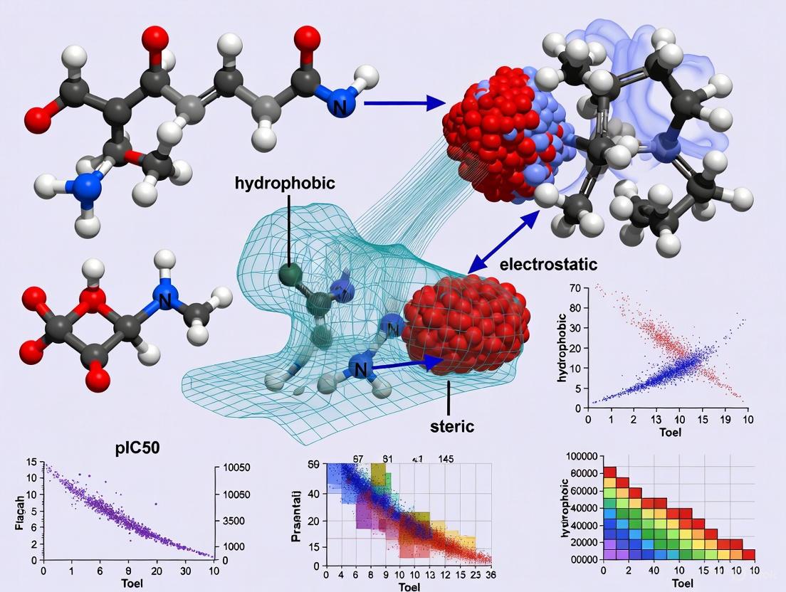
The rational design of anticancer drugs relies on a fundamental understanding of the molecular forces that govern the interaction between a ligand (typically a potential drug molecule) and its biological target (often a protein or enzyme). The biological receptor does not perceive a ligand as a simple set of atoms and bonds; rather, it interacts with a three-dimensional shape that carries a complex distribution of molecular forces [20]. These interactions are determined predominantly by steric (van der Waals), electrostatic (Coulombic), and hydrophobic effects, which collectively determine the binding affinity and specificity of a ligand for its target. Within the framework of Three-Dimensional Quantitative Structure-Activity Relationship (3D-QSAR) modeling, these forces are quantified as molecular fields surrounding the ligand molecules. This methodology is particularly powerful in situations where the detailed three-dimensional structure of the receptor is unknown, as it allows for the correlation of these computed fields with experimentally measured biological activities to guide the optimization of novel therapeutic agents [21] [20].
Fundamental Force Fields and Their Origins
The Steric (Van Der Waals) Field
Steric effects arise from the spatial arrangement of atoms within molecules. When atoms come into close proximity, a rise in the energy of the molecule occurs due to steric hindrance, which is a consequence of the repulsive forces between overlapping electron clouds [22]. These nonbonding interactions profoundly influence the molecular conformation and reactivity. In the context of ligand-target binding, steric forces can be either repulsive or attractive. At very short distances, significant repulsion occurs due to the interpenetration of electronic clouds. At slightly longer ranges, attractive dispersion forces prevail [20]. The steric potential describes these non-electrostatic interactions between non-bonded atoms and is critically important for the final step of binding, as it controls how well the ligand fits into the binding pocket of the target. The associated energy is often calculated using a Lennard-Jones potential, which captures both the repulsive and attractive components of the van der Waals interaction [20].
Table 1: Characteristics of Steric Interactions
| Feature | Description | Impact on Binding |
|---|---|---|
| Origin | Spatial arrangement of atoms and electron clouds [22] | Determines shape complementarity |
| Repulsive Component | Electron cloud overlap at short distances [20] | Prevents unfavorable clashes |
| Attractive Component | Dispersion forces (London forces) at intermediate distances [20] | Provides stabilization energy |
| Distance Dependency | Inverse 12th power (repulsive) [20] | Very short-range effect |
| Probe for 3D-QSAR | Carbon sp³ atom [20] | Maps shape and bulk requirements |
The Electrostatic (Coulombic) Field
Electrostatic interactions occur between polar or charged groups on the ligand and the target. These interactions are governed by Coulomb's law and can be either attractive (between opposite charges) or repulsive (between like charges) [20]. Since the electrostatic energy is expressed as the inverse of the distance between interacting atoms, the electrostatic field exerts influence over relatively long ranges (e.g., 10 angstroms or more). This long-range character means that electrostatic forces often drive the initial approach and orientation of the ligand toward the binding site. The treatment of these interactions in computational models can vary in complexity, from mean-field approaches like Debye-Hückel theory, which uses an implicit screening length, to explicit modeling of all ionic species in solution, with the latter providing more accurate but computationally expensive results [23].
Table 2: Characteristics of Electrostatic Interactions
| Feature | Description | Impact on Binding |
|---|---|---|
| Origin | Charges and polar groups [20] | Guides initial ligand approach |
| Attractive/Repulsive | Opposite charges attract; like charges repel [20] | Provides directionality |
| Distance Dependency | Inverse of the distance (râ»Â¹) [20] | Long-range effect |
| Solvent/Salt Effect | Screening by ionic strength [23] | Modulates interaction strength |
| Probe for 3D-QSAR | Carbon sp³ atom with a +1 charge [20] | Maps charge and polarity requirements |
The Hydrophobic Field
Hydrophobic interactions are a driving force in biomolecular recognition, primarily due to the entropic gain associated with the release of ordered water molecules from hydrophobic surfaces upon ligand binding. These interactions are not attractions between hydrophobic groups per se, but rather the thermodynamic consequence of water molecules reorganizing to minimize their contact with non-polar surfaces. Hydrophobic interactions are a major contributor to binding affinity, and systematic analyses of protein-ligand complexes have shown that hydrophobic contacts are the most common interactions, and are generally enriched in high-efficiency ligands [24]. In fact, the frequency of hydrogen bonds is reduced from 59% to 34% of that of hydrophobic contacts in efficient binders, highlighting the critical role of hydrophobicity in achieving potent binding [24]. The extent of a molecule's hydrophobicity is determined by the number, size, and distribution of hydrophobic patches on its surface, which are special characteristics of each individual protein or ligand [25].
Table 3: Characteristics of Hydrophobic Interactions
| Feature | Description | Impact on Binding |
|---|---|---|
| Origin | Entropic gain from water displacement [25] | Major driving force for binding |
| Solvent Role | Water molecules form cages around non-polar surfaces [25] | The interaction is mediated by solvent |
| Salt Effect | High salt concentration promotes hydrophobic interaction (salting-out) [25] | Can be used to modulate binding |
| Distance Dependency | Complex, based on solvent reorganization | Effective at short to intermediate ranges |
| Prevalence | Most common interaction type in PDB complexes [24] | Critical for high ligand efficiency |
Quantifying Molecular Fields in 3D-QSAR
The Molecular Interaction Field (MIF) Framework
The core principle of 3D-QSAR is the mapping and statistical comparison of the molecular fields surrounding a set of ligand molecules to establish a quantitative relationship with their biological activities [20]. This is achieved by calculating Molecular Interaction Fields (MIFs), which are 3D distributions of interaction energies between a molecule and a chosen probe. To compute these fields, a 3D lattice of grid points is superimposed around the molecule, and the interaction energy between the molecule and the probe is calculated at each grid point using appropriate potential energy functions [20]. This lattice sampling allows for the finite and manageable calculation of MIFs. The resulting fields can be visualized as iso-potential surfaces, which are 3D surfaces connecting all points of the same interaction energy value, providing intuitive, visual insights into the regions where specific interactions favorably or unfavorably influence biological activity.
Diagram 1: 3D-QSAR Field Calculation Workflow. This diagram illustrates the standard computational workflow for deriving a 3D-QSAR model, from ligand preparation through field calculation and statistical analysis.
The Probe Concept and Field Calculation
A probe is a conceptual or computational entity used to test for the presence and strength of a specific molecular field. It is placed at numerous points in the space around a molecule to quantitatively measure the value of the field created by the molecule at each location [20]. The probe must be of the same type as the field to be measured.
- Probing the Steric Field: The steric field is typically probed using a neutral carbon sp³ atom. The interaction energy is calculated at each grid point using a potential function such as the Lennard-Jones 6-12 potential, which captures both the attractive and repulsive components of the van der Waals interaction [20].
- Probing the Electrostatic Field: The electrostatic field is measured using a carbon sp³ atom with a charge of +1. The interaction energy is calculated using Coulomb's law, summing the interactions between the point charge on the probe and the point charges on the atoms of the molecule [20].
- Probing the Hydrophobic Field: While steric and electrostatic probes are standard, the concept can be extended to other fields. Hydrophobic fields, or Molecular Lipophilicity Potentials (MLP), can be calculated using probes representing hydrophobic fragments or based on empirical methods like HINT, which calculates a hydrophobic field from atom-based parameters [20].
The probe concept has been significantly expanded in sophisticated methods like the GRID approach, developed by Peter Goodford. GRID utilizes dozens of chemically realistic probes, including single atoms, water, functional groups (methyl, amine, carbonyl), and even metal cations, to explore the interaction potential of a binding site in great detail [20].
Experimental and Computational Methodologies
Comparative Molecular Similarity Index Analysis (CoMSIA)
The CoMSIA (Comparative Molecular Similarity Index Analysis) method is a powerful and popular 3D-QSAR technique that improves upon earlier methods like CoMFA. A recent study on novel 6-hydroxybenzothiazole-2-carboxamide derivatives as MAO-B inhibitors for neurodegenerative diseases provides an excellent example of a modern CoMSIA application [21].
Protocol:
- Ligand Preparation: A set of compounds with known biological activity (e.g., ICâ‚…â‚€ values) is collected. Their 2D structures are drawn and converted to 3D structures using software like ChemDraw and Sybyl-X. The 3D structures are then energy-minimized to obtain their most stable conformations [21].
- Molecular Alignment: All molecules are superimposed onto a common reference scaffold or a hypothesized pharmacophore model. This alignment is critical, as it assumes that all molecules bind to the target in a similar orientation [21].
- Field Calculation: The CoMSIA method calculates several similarity indices using a common probe. Typically, these include steric, electrostatic, hydrophobic, and hydrogen-bond donor and acceptor fields [21].
- Statistical Analysis: The calculated field values for all compounds are compiled into a data matrix. Partial Least Squares (PLS) regression is used to correlate the field descriptors with the biological activity values. The model is validated using techniques like leave-one-out (LOO) cross-validation, yielding predictive metrics such as q² (cross-validated correlation coefficient) and r² (non-cross-validated correlation coefficient) [21]. In the cited study, the CoMSIA model exhibited a q² of 0.569 and an r² of 0.915, indicating a model with good predictive ability and high statistical significance [21].
Molecular Docking and Dynamics
Molecular docking and dynamics (MD) simulations are complementary techniques used to understand the stability and detailed mechanics of ligand-target interactions predicted by 3D-QSAR models.
Protocol:
- Molecular Docking: The most promising compounds identified from the 3D-QSAR analysis are subjected to molecular docking into the binding site of the target protein (e.g., MAO-B). Software such as Discovery Studio (LigandFit, CDOCKER) or AutoDock is used for this purpose. Docking predicts the preferred orientation (pose) of the ligand and provides a docking score representing the estimated binding affinity [21] [26].
- Molecular Dynamics Simulation: To assess the stability of the docked complex under more realistic conditions, MD simulations are performed (e.g., for 100 nanoseconds). The complex is solvated in a water box, ions are added to neutralize the system, and Newton's equations of motion are solved over time. Key analyzed parameters include:
- Root Mean Square Deviation (RMSD): Measures the stability of the protein-ligand complex. Stable binding is indicated by RMSD values fluctuating within a small range (e.g., 1.0-2.0 Ã…) [21].
- Binding Free Energy Calculations: Methods like Molecular Mechanics/Generalized Born Surface Area (MM/GBSA) are used to calculate the binding free energy, decomposing it into contributions from van der Waals, electrostatic, and solvation energies [21].
- Energy Decomposition: This analysis reveals the contribution of key amino acid residues to the total binding energy, identifying which residues are most critical for stabilizing the complex through various interaction types [21].
Analysis of Protein-Ligand Interaction Databases
A systematic, large-scale analysis of experimentally determined protein-ligand structures provides statistically robust insights into the real-world prevalence and impact of different interaction types.
Protocol:
- Data Curation: A non-redundant set of high-resolution (e.g., ≤2.5 Å) X-ray structures of protein-ligand complexes is compiled from the Protein Data Bank (PDB). Ligands are filtered to include only medicinally relevant small molecules, excluding buffers and crystallization additives [24].
- Interaction Detection: Software tools and algorithms (e.g., PDBeMotif, PELIKAN) are used to automatically identify and classify atomic interactions (e.g., hydrophobic, hydrogen bond, salt bridge, π-stacking) based on predefined geometric criteria (e.g., atom pairs within 4.0 Å) [24].
- Frequency and Efficiency Analysis: The frequency of each interaction type is calculated across the entire dataset. To understand which interactions correlate with strong binding, ligands can be ranked by a Fit Quality (FQ) score (a size-adjusted measure of ligand efficiency), and the interaction patterns of the top and bottom performers are compared [24]. This analysis quantitatively demonstrates that hydrophobic interactions are more frequent in high-efficiency ligands [24].
Table 4: Essential Resources for 3D-QSAR and Interaction Analysis
| Category | Item / Software | Function / Application |
|---|---|---|
| Software Suites | Sybyl-X [21] | Comprehensive molecular modeling and 3D-QSAR (e.g., CoMSIA). |
| Discovery Studio (LigandFit, CDOCKER) [26] | Molecular docking and simulation studies. | |
| GRID [20] | Structure-based analysis of binding sites using multiple probes. | |
| Databases | Protein Data Bank (PDB) [24] | Source of 3D protein-ligand complex structures for analysis and docking. |
| PDBbind [24] | Curated database of binding affinities for structures in the PDB. | |
| Computational Probes | C sp³ (neutral) [20] | Standard probe for calculating steric molecular fields. |
| C sp³ (+1 charge) [20] | Standard probe for calculating electrostatic molecular fields. | |
| Water, Methyl, Amine, Carboxylate [20] | Multi-atom probes in GRID for mapping specific functional group interactions. | |
| Analysis Tools | LigPlot [26] | Generates 2D diagrams of ligand-protein interactions. |
| VMD [20] | Visualization and analysis of molecular dynamics trajectories. |
Steric, electrostatic, and hydrophobic fields form the foundational triad of molecular interactions that control ligand-target recognition and binding affinity. In the context of anticancer drug design, the ability to quantify and model these forces through 3D-QSAR approaches like CoMSIA provides a powerful, rational framework for optimizing lead compounds. Integrating these methods with molecular docking, dynamics simulations, and large-scale bioinformatic analyses of structural databases creates a robust pipeline for modern drug discovery. The insights gained—such as the primacy of hydrophobic interactions in high-efficiency binders and the critical balance between long-range electrostatic steering and short-range steric complementarity—provide medicinal chemists with a strategic roadmap. By systematically applying these principles, researchers can more efficiently navigate the chemical space toward novel, potent, and selective anticancer therapeutics.
The Critical Role of 3D-QSAR in Targeting Key Cancer Proteins and Pathways
In modern anticancer drug design, the complexity of cancer biology demands strategies that can overcome the limitations of single-target therapies, which often fail due to compensatory pathways and drug resistance. Three-dimensional Quantitative Structure-Activity Relationship (3D-QSAR) modeling has emerged as a pivotal computational approach that addresses this challenge by enabling the rational design of multi-target inhibitors. Unlike traditional QSAR methods that rely on two-dimensional molecular descriptors, 3D-QSAR incorporates the critical three-dimensional structural characteristics of molecules, providing superior predictive ability for biological activity based on conformational and steric properties [9]. This advanced methodology allows medicinal chemists to visualize the interaction fields between ligands and target proteins, facilitating the optimization of compound structures for enhanced potency and selectivity against key cancer targets.
The foundational 3D-QSAR techniques, primarily Comparative Molecular Field Analysis (CoMFA) and Comparative Molecular Similarity Indices Analysis (CoMSIA), have revolutionized computer-aided drug design by establishing reliable correlations between molecular structure variations and biological activity [27] [9]. These approaches have become indispensable in oncology drug discovery, particularly for designing compounds that simultaneously inhibit multiple cancer-related proteins and pathways. By leveraging 3D-QSAR insights, researchers can efficiently prioritize the most promising candidate molecules for synthesis and biological testing, significantly accelerating the drug development pipeline while reducing associated costs and resource expenditures [9].
Key Cancer Targets and Multi-Target Inhibition Strategies
Critical Proteins in Cancer Progression
Cancer pathogenesis involves multiple interconnected signaling pathways and regulatory proteins that collectively drive tumor development and progression. Key among these are cyclin-dependent kinase 2 (CDK2), which regulates cell cycle progression; epidermal growth factor receptor (EGFR), a critical mediator of cell proliferation and survival signals; and tubulin, whose polymerization dynamics are essential for mitotic spindle formation and cell division [28]. Simultaneous inhibition of these strategically selected targets presents a powerful approach to disrupt cancer cell viability while mitigating the development of resistance commonly observed with single-target agents [28].
Other significant targets in cancer therapy include glycogen synthase kinase-3β (GSK-3β), which is implicated in multiple signaling pathways and represents a promising target particularly in therapeutic areas beyond oncology, and monoamine oxidase B (MAO-B), which has been explored in neurodegenerative diseases but demonstrates the broader applicability of 3D-QSAR methodologies [27] [9]. The multi-target inhibition strategy leverages the polypharmacology concept, where single chemical entities are designed to interact with multiple specific targets simultaneously, providing enhanced therapeutic efficacy compared to monotherapies or drug combinations [28].
Established Multi-Target Inhibitors in Cancer Research
Table 1: Representative Multi-Target Inhibitors Designed Using 3D-QSAR Approaches
| Compound Class | Key Targets | Cancer Type | Binding Affinity (kcal/mol) | Reference Compound |
|---|---|---|---|---|
| Phenylindole derivatives | CDK2, EGFR, Tubulin | Breast Cancer (MCF-7) | -7.2 to -9.8 | Molecule 39 |
| 6-Hydroxybenzothiazole-2-carboxamides | MAO-B | Neurodegenerative diseases (demonstrating methodology) | N/A | Selegiline, Rasagiline |
| Oxadiazole derivatives | GSK-3β | Alzheimer's disease (demonstrating methodology) | N/A | N/A |
Recent studies have demonstrated the successful application of 3D-QSAR in designing phenylindole derivatives that concurrently inhibit CDK2, EGFR, and tubulin [28]. These novel compounds exhibited superior binding affinities ranging from -7.2 to -9.8 kcal/mol compared to reference drugs, highlighting the power of structure-based design in developing potent multi-target agents [28]. The integration of computational predictions with experimental validation has accelerated the identification of promising chemotypes with balanced potency across multiple targets, addressing a significant challenge in multi-target drug development.
3D-QSAR Methodologies: Experimental Protocols and Workflows
Core Computational Protocols
The implementation of robust 3D-QSAR models follows a systematic workflow that ensures predictive accuracy and reliability. The following diagram illustrates the standard experimental protocol for 3D-QSAR model development and application:
Dataset Preparation and Molecular Modeling
The initial phase involves curating a diverse set of compounds with experimentally determined biological activities (ICâ‚…â‚€ or Ki values), which are typically converted to pICâ‚…â‚€ (-log ICâ‚…â‚€) for modeling [27]. Molecular structures are constructed using chemical drawing software such as ChemDraw and optimized for geometry and energy minimization using molecular modeling packages like Sybyl-X [9]. Proper molecular alignment through pharmacophore-based or docking-based methods is crucial, as the predictive power of 3D-QSAR models depends significantly on correct spatial orientation of the molecules in three-dimensional space.
Field Calculation and Model Construction
CoMFA calculates steric (Lennard-Jones potential) and electrostatic (Coulombic potential) fields around each molecule, while CoMSIA extends this approach to include additional similarity indices such as hydrophobic, hydrogen bond donor, and hydrogen bond acceptor fields [27]. These field values serve as independent variables in Partial Least Squares (PLS) regression analysis to establish the correlation with biological activity. The dataset is typically divided into training sets (for model development) and test sets (for external validation), ensuring structural diversity and representative activity distribution across both sets [27].
Model Validation and Contour Map Interpretation
Rigorous validation is essential for reliable 3D-QSAR models. Internal validation employs leave-one-out cross-validation, yielding the Q² value (cross-validated correlation coefficient), while external validation uses the test set to calculate R²ₚᵣₑd (predictive correlation coefficient) [28] [27]. High-quality models typically demonstrate Q² > 0.5 and R²ₚᵣₑd > 0.6, with recent studies reporting exceptional values of Q² = 0.814 and R²ₚᵣₑd = 0.722 for phenylindole derivatives targeting cancer proteins [28]. The resulting contour maps visualize regions where specific structural modifications would enhance or diminish biological activity, providing medicinal chemists with clear guidance for molecular design.
Research Reagent Solutions: Essential Tools for 3D-QSAR Implementation
Table 2: Essential Computational Tools and Their Applications in 3D-QSAR Studies
| Tool Category | Specific Software/Platform | Primary Function | Application in Workflow |
|---|---|---|---|
| Molecular Modeling | Sybyl-X | Structure building, optimization, and QSAR modeling | Core 3D-QSAR model development |
| Molecular Modeling | ChemDraw | Chemical structure drawing and representation | Initial structure creation |
| Docking & Visualization | Molegro Virtual Docker | Virtual screening and binding affinity assessment | Post-QSAR validation |
| Docking & Visualization | Discovery Studio | Protein-ligand interaction analysis and RMSD calculation | Binding mode analysis |
| Descriptor Calculation | Dragon Software | Molecular descriptor computation | Additional QSAR descriptors |
| Dynamics Simulation | GROMACS, AMBER | Molecular dynamics simulations | Binding stability assessment |
Successful implementation of 3D-QSAR studies requires integration of specialized software tools that cover the entire workflow from initial structure preparation to final validation. Commercial molecular modeling suites like Sybyl-X provide comprehensive environments for CoMFA and CoMSIA model development [9], while virtual screening platforms such as Molegro Virtual Docker enable assessment of binding affinities for designed compounds [29]. Molecular dynamics simulations using packages like GROMACS or AMBER provide critical insights into the stability and dynamic behavior of protein-ligand complexes over time, typically through 100ns simulation trajectories that evaluate root mean square deviation (RMSD) and binding free energies [28].
Case Studies: Successful Application in Cancer Drug Discovery
Phenylindole Derivatives as Multi-Target Inhibitors
A recent investigation demonstrated the power of 3D-QSAR in designing phenylindole derivatives as simultaneous inhibitors of CDK2, EGFR, and tubulin for breast cancer therapy [28]. The established CoMSIA/SEHDA model exhibited exceptional statistical reliability with R² = 0.967 and Q² = 0.814, enabling the design of six novel compounds with predicted enhanced activity [28]. Molecular docking confirmed superior binding affinities (-7.2 to -9.8 kcal/mol) compared to reference compounds, while molecular dynamics simulations over 100ns verified complex stability [28]. This case highlights how 3D-QSAR can guide the development of single agents capable of disrupting multiple cancer pathways simultaneously, addressing the critical challenge of drug resistance.
Oxadiazole Derivatives as GSK-3β Inhibitors
While primarily investigated for Alzheimer's disease, the development of oxadiazole derivatives as GSK-3β inhibitors exemplifies methodology transferable to cancer research, particularly given GSK-3β's role in oncogenic signaling [27]. The constructed CoMFA (R²cv = 0.692, R²pred = 0.6885) and CoMSIA (R²cv = 0.696, R²pred = 0.6887) models successfully identified critical structural features influencing inhibitory activity [27]. Molecular docking and dynamics simulations further elucidated key interactions with residues Ile62, Asn64, Val70, Tyr128, Val129, and Leu182 in the GSK-3β active site [27]. This systematic approach demonstrates how 3D-QSAR contour maps can direct specific molecular modifications to enhance target engagement.
Integration with Complementary Computational Methods
Molecular Docking and Dynamics Simulations
3D-QSAR predictions gain significant robustness when integrated with complementary computational approaches. Molecular docking provides atomic-level insights into binding modes and protein-ligand interactions, validating that compounds designed using 3D-QSAR contours favorably occupy target binding sites [28] [9]. Molecular dynamics simulations extending to 100ns further assess complex stability, conformational fluctuations, and interaction persistence under biologically relevant conditions [28]. The following diagram illustrates how these methodologies are integrated in a comprehensive drug design pipeline:
Binding Free Energy Calculations and ADMET Profiling
Advanced energy calculations using Molecular Mechanics Generalized Born Surface Area (MM-GBSA) or Poisson-Boltzmann Surface Area (MM-PBSA) methods provide quantitative estimates of binding affinities, complementing the qualitative insights from docking studies [29]. Additionally, absorption, distribution, metabolism, excretion, and toxicity (ADMET) profiling predicts pharmacological and safety properties of designed compounds prior to synthesis, with recent studies confirming favorable ADMET profiles for 3D-QSAR-designed candidates [28]. This multi-faceted computational approach significantly de-risks the drug discovery process by ensuring that only compounds with optimal activity, selectivity, and drug-like properties advance to experimental evaluation.
3D-QSAR methodologies have firmly established their critical role in modern anticancer drug design, particularly for developing multi-target agents that address the complex pathophysiology of cancer. The integration of CoMFA/CoMSIA with molecular docking, dynamics simulations, and ADMET prediction creates a powerful computational framework that accelerates the identification of promising therapeutic candidates. As structural biology advances provide more high-resolution target structures, and machine learning algorithms enhance model precision, 3D-QSAR approaches will continue to evolve in sophistication and predictive accuracy. The ongoing development of 3D-QSAR methodologies promises to significantly impact oncology drug discovery by enabling more efficient, targeted, and rational design of next-generation multi-target anticancer therapeutics.
Implementing 3D-QSAR: A Step-by-Step Guide to Model Building and Application
In the field of anticancer drug design, the development of predictive and reliable three-dimensional Quantitative Structure-Activity Relationship (3D-QSAR) models is fundamentally dependent on the quality of the underlying compound data. Data curation, the process of preparing and preprocessing chemical datasets, transforms raw, often inconsistent biological screening data into a structured, validated resource suitable for computational modeling. Within the context of 3D-QSAR, which quantitatively correlates the three-dimensional molecular properties of compounds with their biological activity, rigorous data curation is not merely a preliminary step but a critical determinant of model success [30] [31].
The core objective of 3D-QSAR is to construct a predictive model that can guide the rational design of novel drug candidates, for instance, by identifying key steric and electrostatic features essential for inhibiting a specific anticancer target [5] [31]. These models, such as Comparative Molecular Field Analysis (CoMFA) and Comparative Molecular Similarity Indices Analysis (CoMSIA), are highly sensitive to the input data's consistency and accuracy. A model built on a poorly curated dataset will generate misleading contours, resulting in incorrect structural interpretations and ultimately, the costly synthesis of inactive compounds. Therefore, a meticulously curated dataset is the bedrock upon which robust, interpretable, and predictive 3D-QSAR models are built, directly impacting the efficiency of the anticancer drug discovery pipeline.
Foundational Concepts: From Biological Endpoints to Molecular Descriptors
Quantitative Biological Activity Data
The biological activity of compounds must be expressed in a consistent, quantitative manner to serve as the dependent variable in a QSAR model. For anticancer drug discovery, common measurements include:
- ICâ‚…â‚€: The concentration of a compound required to inhibit 50% of a target enzyme's activity or 50% of cell proliferation in vitro [31].
- ECâ‚…â‚€: The concentration of an agonist required to produce 50% of the maximum possible response [31].
- Káµ¢: The enzyme inhibition constant, representing the affinity of an inhibitor for an enzyme [31].
These continuous values are typically converted into pICâ‚…â‚€ or pKáµ¢ (pICâ‚…â‚€ = -logICâ‚…â‚€) for use in QSAR modeling, which linearizes the relationship with free energy changes [5] [9].
Molecular Descriptors in 3D-QSAR
Unlike 2D-QSAR, which uses molecular descriptors derived from the two-dimensional structure, 3D-QSAR relies on properties calculated from the three-dimensional conformation of molecules. The most common descriptors are fields representing non-covalent interaction energies:
- Steric Fields: Represent the Lennard-Jones potential, modeling repulsive and attractive van der Waals forces [31].
- Electrostatic Fields: Represent the Coulombic potential, modeling favorable and unfavorable charge interactions [31].
- Additional CoMSIA Fields: Hydrophobic, and Hydrogen Bond Donor and Acceptor fields provide a more comprehensive profile of interaction potentials [31].
Table 1: Key Biological Endpoints and Descriptors in QSAR Modeling
| Category | Parameter | Description | Role in QSAR |
|---|---|---|---|
| Biological Endpoints | ICâ‚…â‚€ / pICâ‚…â‚€ | Half-maximal inhibitory concentration / its negative logarithm | Primary dependent variable; represents potency |
| Káµ¢ / pKáµ¢ | Enzyme inhibition constant / its negative logarithm | Represents binding affinity | |
| GIâ‚…â‚€ | Concentration for 50% inhibition of cell proliferation | Used in cellular-level activity models | |
| 3D-QSAR Descriptors | Steric Fields (CoMFA/CoMSIA) | Lennard-Jones potential around the molecule | Models shape complementarity and steric clashes |
| Electrostatic Fields (CoMFA/CoMSIA) | Coulombic potential around the molecule | Models charge-charge interactions | |
| Hydrophobic Fields (CoMSIA) | Atom-based hydrophobicity parameters | Models desolvation and entropic effects |
A Systematic Workflow for Data Curation and Preprocessing
A standardized workflow for data curation ensures the integrity and usability of a compound dataset for 3D-QSAR analysis. The following diagram outlines the critical stages from raw data collection to a curated dataset ready for modeling.
Stage 1: Activity Data Curation
The initial phase focuses on the biological data, ensuring it is reliable, consistent, and suitable for modeling.
- Data Sourcing and Aggregation: Gather data from internal high-throughput screens, public databases, and scientific literature. A typical dataset for a robust 3D-QSAR model should contain a minimum of 20-50 diverse compounds with reliably measured activity values [31]. For example, a study on Bcr-Abl inhibitors for leukemia curated a dataset of 58 purine derivatives with reported ICâ‚…â‚€ values [5].
- Unit Standardization and Homogenization: Convert all activity values into a single, consistent unit and scale (e.g., nanomolar to molar, then to pICâ‚…â‚€). This step is crucial when merging data from multiple sources.
- Outlier Identification and Justification: Statistically identify and critically evaluate compounds with aberrant activity values. Outliers may be removed if they are attributed to experimental error, or they may be retained if they represent a unique and important structure-activity relationship, with the rationale documented.
Stage 2: Chemical Structure Curation
This stage ensures the digital representation of each molecule is accurate and standardized.
- Structure Representation and Tautomer Standardization: Define and apply consistent rules for protonation states, tautomeric forms, and charges at a defined pH (e.g., pH 7.4). This is critical as different representations can lead to vastly different 3D field calculations.
- Descriptor Verification and Inorganic Counterion Removal: Check for and correct errors in atom types and valences. Remove simple salts and inorganic counterions (e.g., Naâº, Clâ») from the molecular structure, as they are not relevant for the target interaction but can distort field calculations.
Stage 3: 3D Conformation Generation and Alignment
This is the most distinctive and critical stage for 3D-QSAR, as the model's output is directly contingent on the spatial alignment of the molecules.
- 3D Conformation Generation and Low-Energy Conformer Selection: Use reliable algorithms (e.g., within Sybyl, OpenEye toolkits) to generate 3D structures from 2D representations. For flexible molecules, it is essential to identify and use the putative bioactive conformation. This can be achieved by selecting a low-energy conformer that is similar to a known crystallographic ligand or by using a common scaffold-based alignment rule [31] [9].
- Molecular Alignment Based on a Rational Hypothesis: Align all molecules in the dataset according to a consistent strategy. Common methods include:
- Pharmacophore-based alignment: Using a set of common functional groups presumed to be critical for binding.
- Database alignment: Superimposing molecules onto the structure of a known active compound or a template molecule.
- Ligand-based alignment: Using the maximum common substructure (MCS) as the template for superposition [31]. The choice of alignment strategy is a key hypothesis in the 3D-QSAR model construction.
Experimental Protocol: A Case Study on Kinase Inhibitors
The following detailed protocol is adapted from a recent study that developed 3D-QSAR models for purine-based Bcr-Abl inhibitors, a relevant class of anticancer agents for chronic myeloid leukemia [5].
Materials and Computational Tools
Table 2: Research Reagent Solutions for 3D-QSAR Data Curation
| Item/Category | Specific Examples & Versions | Primary Function in Workflow |
|---|---|---|
| Chemical Modeling Software | Sybyl-X, Molecular Operating Environment (MOE), Schrodinger Maestro | Integrated platform for structure building, conformational analysis, molecular alignment, and CoMFA/CoMSIA analysis. |
| Structure Drawing/Preparation | ChemDraw | Primary tool for drawing and standardizing 2D chemical structures prior to 3D conversion. |
| Conformation Generation Algorithm | CORINA, OMEGA | Algorithms used to convert 2D structures into accurate 3D conformations and search low-energy conformational space. |
| Activity Data Source | Internal HTS, PubChem BioAssay, ChEMBL | Public and proprietary databases providing experimental ICâ‚…â‚€ or Káµ¢ values for model training and validation. |
| Scripting & Automation | Python (RDKit, Pandas), R | Custom scripts for automating repetitive curation tasks like file format conversion, unit standardization, and data filtering. |
Step-by-Step Methodology
Compound Dataset Assembly:
- Source: A dataset of 58 known 2,6,9-trisubstituted purine derivatives with reported Bcr-Abl inhibitory activity (ICâ‚…â‚€) was assembled from the literature [5].
- Curation Action: All ICâ‚…â‚€ values were converted to pICâ‚…â‚€ (-logICâ‚…â‚€) to create a linear, modeling-friendly activity parameter.
Chemical Structure Preparation and Optimization:
- Tools: 2D structures of all compounds were drawn using ChemDraw and subsequently imported into Sybyl-X software for 3D optimization [5].
- Curation Action: The common purine scaffold was identified. Structures were energy-minimized using the Tripos force field and Gasteiger-Hückel partial atomic charges were calculated to prepare for field computations.
Molecular Alignment:
- Strategy: A ligand-based alignment strategy was employed.
- Curation Action: The purine core of all 58 molecules was used as the common substructure for superposition. Each molecule was aligned to this template to ensure all compounds were in a consistent frame of reference, a prerequisite for calculating comparable molecular fields [5].
3D-QSAR Model Construction and Validation:
- Analysis: The aligned molecule set was placed in a 3D grid, and steric (Lennard-Jones) and electrostatic (Coulombic) field energies were computed at each grid point using a sp³ carbon probe atom.
- Validation: The model was built using the CoMFA method. Its predictive ability was rigorously validated. The study reported a cross-validated coefficient (q²) of 0.569 and a non-cross-validated coefficient (r²) of 0.915, indicating a highly robust and predictive model [5]. This validation is a direct reflection of a well-curated underlying dataset.
Data curation is an indispensable, multi-faceted process that transforms disparate chemical and biological data into a foundational resource for predictive 3D-QSAR modeling. By adhering to a rigorous workflow encompassing activity data standardization, chemical structure validation, and rational molecular alignment, researchers can construct datasets of the highest integrity. As demonstrated in the anticancer kinase inhibitor case study, such meticulous preparation directly enables the development of robust 3D-QSAR models with high predictive power. These models provide invaluable, actionable insights into the structural determinants of biological activity, thereby accelerating the rational design of novel, potent, and selective anticancer therapeutics.
In the realm of computer-aided drug design, particularly in anticancer research, three-dimensional quantitative structure-activity relationship (3D-QSAR) modeling serves as a powerful predictive tool for optimizing lead compounds. Unlike traditional 2D-QSAR methods that use numerical descriptors invariant to molecular conformation, 3D-QSAR incorporates spatial structural information, considering the molecule as a 3D object with specific shape and interaction potentials [32]. The fundamental principle underpinning 3D-QSAR is that biological activity correlates with molecular interaction fields surrounding the compound, which are intrinsically tied to their three-dimensional orientation [31].
Molecular alignment constitutes the most critical and technically demanding step in the 3D-QSAR workflow. The process involves superimposing all molecules within a shared 3D reference frame that reflects their putative bioactive conformations [32]. Imagine comparing keys by aligning them to fit the same lock; similarly, in 3D-QSAR, researchers must select a bioactive conformation for each molecule and align all compounds to a common orientation. The quality of this alignment directly determines the predictive accuracy and interpretability of the resulting model, as misaligned molecules generate inconsistent descriptor values that obscure true structure-activity relationships [32] [6].
Core Alignment Methodologies in Anticancer Drug Design
The strategic selection of an alignment protocol depends on available structural information, dataset diversity, and the specific biological target. The following methodologies represent the principal approaches employed in 3D-QSAR studies for anticancer research.
Ligand-Based Alignment Approaches
Pharmacophore-Based Alignment utilizes a common pharmacophore hypothesis as a template for superposition. This approach identifies the spatial arrangement of chemical features essential for biological activity, such as hydrogen bond acceptors/donors, hydrophobic regions, and aromatic rings [10]. In a study on cytotoxic quinolines as tubulin inhibitors, researchers identified a six-point pharmacophore model (AAARRR.1061) consisting of three hydrogen bond acceptors and three aromatic rings [10]. Compounds were aligned to this hypothesis to ensure consistent spatial orientation for 3D-QSAR analysis, enabling the identification of critical structural features governing anticancer activity.
Maximum Common Substructure (MCS) Alignment identifies the largest substructure shared among all molecules in the dataset [32]. Alignment is achieved by superimposing this common framework, particularly useful for datasets with significant structural diversity where defined scaffolds may not exist. This method facilitates meaningful comparison across varied chemotypes by focusing alignment on the most significant common features [32].
Structure-Based and Field-Based Approaches
Template-Based Alignment uses a known active compound or reference structure as a template. In investigations of maslinic acid analogs for breast cancer activity against MCF-7 cells, the FieldTemplater module identified a hypothesis for the 3D conformation using field and shape information from selected active compounds [6]. The resulting field point pattern provided a condensed representation of shape, electrostatics, and hydrophobicity, serving as an alignment template that presumably resembles the bioactive conformation [6].
Field-Based Alignment employs molecular field similarity rather than atomic positions for superposition. This approach can be particularly valuable when dealing with structurally diverse compounds that share similar interaction patterns with biological targets, as it focuses on similarity in interaction potentials rather than strict atomic correspondence [6].
Advanced and Alignment-Independent Methods
Docking-Based Alignment utilizes computational docking to align molecules into a protein's binding site. This structure-based approach provides a biologically relevant orientation when the target protein structure is known, theoretically reflecting the actual binding mode [10] [6]. However, its accuracy depends heavily on the precision of the docking algorithm and scoring functions.
Alignment-Independent 3D-QSDAR represents a paradigm shift that circumvents alignment challenges. The 3D-QSDAR (Quantitative Spectral Data-Activity Relationship) technique uses NMR chemical shifts and interatomic distances to create unique molecular fingerprints independent of spatial alignment [33]. Remarkably, a study on androgen receptor binders found that simple 2D-to-3D converted structures performed equally well or better than carefully aligned conformations, achieving excellent predictive accuracy in significantly less computational time [33].
Table 1: Comparison of Molecular Alignment Methodologies in 3D-QSAR
| Method | Key Principle | Best Use Cases | Advantages | Limitations |
|---|---|---|---|---|
| Pharmacophore-Based | Alignment to essential chemical features | Diverse compounds sharing key pharmacophoric elements | Directly links features to activity; interpretable | Requires reliable pharmacophore model |
| MCS-Based | Superposition of largest common substructure | Structurally related but diverse compounds | Handles scaffold variations; automated | Performance degrades with low similarity |
| Template-Based | Superposition to reference molecule | Congeneric series with clear lead compound | Simple implementation; intuitive | Bias toward template conformation |
| Field-Based | Molecular field similarity | Structurally diverse compounds with similar fields | Captures interaction potential; not atom-based | Computationally intensive; complex interpretation |
| Docking-Based | Alignment in protein binding site | Known protein structure; diverse binders | Biologically relevant; structure-based | Dependent on docking accuracy |
| Alignment-Independent 3D-QSDAR | Uses spectral coordinates and distances | Large datasets; flexible molecules | No alignment needed; fast execution | Limited to available atomic properties |
Experimental Protocols and Workflow Implementation
The practical implementation of molecular alignment follows a systematic workflow that integrates multiple computational steps to ensure biologically relevant results.
Comprehensive Alignment Workflow
The diagram below illustrates the standard decision pathway for selecting and implementing molecular alignment strategies in anticancer drug design:
Practical Implementation Protocols
Protocol 1: Pharmacophore-Based Alignment for Tubulin Inhibitors This protocol was successfully applied in a 3D-QSAR study of quinolines as tubulin inhibitors with anticancer activity [10]:
- Conformational Sampling: Generate multiple low-energy conformations for each compound using appropriate methods (e.g., Monte Carlo, systematic search)
- Pharmacophore Generation: Identify common chemical features from active compounds using software such as Phase or FieldTemplater
- Feature Mapping: Define pharmacophore elements (hydrogen bond acceptors, aromatic rings, hydrophobic regions)
- Molecular Superposition: Align compounds by matching pharmacophore points using rigid or flexible alignment algorithms
- Quality Assessment: Evaluate alignment quality through RMSD measurements and visual inspection
Protocol 2: Field-Based Alignment for Maslinic Acid Analogs In a breast cancer study targeting MCF-7 cells, researchers implemented this protocol [6]:
- Template Selection: Identify active compounds representing diverse structural features for template generation
- Field Calculation: Compute molecular fields (electrostatic, steric, hydrophobic) using extended electron distribution force fields
- Field Point Generation: Derive field points representing regions of significant molecular interaction potential
- Similarity Optimization: Align compounds by maximizing field similarity scores rather than atomic position overlap
- Validation: Verify alignment through activity correlation and contour map interpretability
Protocol 3: Alignment-Independent 3D-QSDAR Implementation For large datasets of flexible compounds, this protocol offers an efficient alternative [33]:
- Structure Conversion: Convert 2D structures to 3D coordinates using standard molecular mechanics
- Descriptor Calculation: Compute 3D-SDAR descriptors using NMR chemical shifts and interatomic distances without alignment
- Grid Generation: Tessellate the 3D-SDAR space into regular bins for descriptor calculation
- Model Building: Employ partial least squares (PLS) regression with multiple training/test randomization cycles
- Consensus Modeling: Average predictions from models built on different conformations for enhanced accuracy
Validation and Impact Assessment of Alignment Strategies
Quantitative Validation of Alignment Quality
The critical importance of molecular alignment is substantiated by comparative studies evaluating different conformational strategies. A comprehensive investigation on 146 androgen receptor binders revealed striking performance differences based on alignment approaches [33]:
Table 2: Performance Comparison of Alignment Strategies in 3D-QSAR Modeling
| Alignment Strategy | Average R²test | Computational Time | Key Applications | Notable Findings |
|---|---|---|---|---|
| Energy-Minimized Conformations | 0.56-0.61 | 100% (Reference) | Standard practice for congeneric series | Good performance but computationally expensive |
| Systematic Template Alignment | 0.56-0.61 | Similar to energy minimization | Targets with known active templates | No significant advantage over simple minimization |
| 2D→3D Conversion (Non-optimized) | 0.61 | 3-7% of reference time | Large datasets; nuclear receptor targets | Superior predictive ability with massive time savings |
| Consensus Models (Multiple Conformations) | 0.65 | 150-200% of reference time | Critical applications requiring high accuracy | Best overall performance through ensemble averaging |
The unexpected superiority of simple 2D-to-3D conversion for certain target classes underscores the context-dependent nature of alignment strategy selection. This approach proved particularly effective for endocrine system nuclear receptors and other targets where strongest activities are produced by fairly inflexible substrates [33].
Impact on Model Interpretation in Anticancer Design
Proper molecular alignment directly enables meaningful interpretation of 3D-QSAR contour maps, which guide rational drug design in anticancer research. In the maslinic acid study, correctly aligned models produced interpretable contour maps that identified specific regions where steric bulk enhanced or diminished activity against breast cancer cells [6]. Similarly, for quinoline-based tubulin inhibitors, the pharmacophore-based alignment revealed favorable hydrophobic regions and essential hydrogen bonding features critical for maintaining anticancer activity [10].
Misalignment, conversely, introduces noise that obscures legitimate structure-activity relationships. Even minor misalignments can significantly degrade model quality, particularly for alignment-sensitive techniques like CoMFA (Comparative Molecular Field Analysis) [32]. The consistency of molecular superposition ensures that steric and electrostatic descriptors calculated at grid points reflect genuine molecular differences rather than alignment artifacts.
Successful implementation of molecular alignment strategies requires specialized software tools and computational resources. The following table catalogs essential components of the alignment toolkit for 3D-QSAR researchers in anticancer drug discovery:
Table 3: Essential Research Reagents and Computational Tools for Molecular Alignment
| Resource Category | Specific Tools/Platforms | Primary Function in Alignment | Application Context |
|---|---|---|---|
| Molecular Modeling Suites | Schrodinger Suite, SYBYL, ChemBio3D | 3D structure generation and optimization | Foundation for all alignment methods; conformational analysis |
| Pharmacophore Modeling | Phase (Schrodinger), FieldTemplater (Cresset) | Pharmacophore hypothesis generation and alignment | Ligand-based alignment for diverse compounds |
| Field-Based Alignment | Forge (Cresset), Open3DALIGN | Molecular field calculation and similarity optimization | Alignment of structurally diverse compounds with similar fields |
| Docking Software | Glide, AutoDock, GOLD | Structure-based alignment into binding sites | Targets with known protein structures |
| Open-Cheminformatics | RDKit, OpenBabel | Maximum common substructure identification and alignment | Cost-effective implementation of MCS-based methods |
| Alignment-Independent | Custom 3D-QSDAR implementations | Spectral coordinate-based descriptor calculation | Large datasets of flexible molecules; rapid screening |
| Conformational Sampling | MacroModel, CONFGEN, OMEGA | Comprehensive conformational space exploration | Essential preprocessing for all alignment methods |
| Visualization & Validation | PyMOL, Maestro, VMD | Visual assessment of alignment quality | Critical for quality control and result interpretation |
Molecular alignment remains the cornerstone of successful 3D-QSAR modeling in anticancer drug design. The selection of an appropriate alignment strategy must consider dataset characteristics, available structural information, and the specific biological target. While traditional alignment-dependent methods continue to provide valuable insights, emerging alignment-independent approaches like 3D-QSDAR offer compelling advantages for large-scale applications involving flexible molecules [33].
Future developments will likely focus on hybrid approaches that combine the interpretability of traditional alignment with the efficiency of alignment-independent methods. The integration of machine learning techniques may further refine alignment strategies by identifying optimal conformational representatives and alignment rules directly from biological activity data [34]. As anticancer drug discovery confronts increasingly challenging targets, advances in molecular alignment will continue to enhance the predictive power and practical utility of 3D-QSAR models in developing novel therapeutic agents.
Comparative Molecular Field Analysis (CoMFA) for Steric and Electrostatic Mapping
Comparative Molecular Field Analysis (CoMFA) represents a pivotal advancement in three-dimensional quantitative structure-activity relationship (3D-QSAR) modeling that has transformed modern drug design. Developed by Cramer et al. in 1988, CoMFA provides a sophisticated approach to correlate biological activity with molecular structural features in three-dimensional space, offering significant advantages over traditional 2D-QSAR methods [35]. The fundamental premise of CoMFA is that the biological activity of molecules typically depends on complementary noncovalent interactions—primarily steric (van der Waals) and electrostatic (Coulombic) forces—with their biological targets [35]. This technique creates a type of 3D contour map of the physicochemical forces surrounding a series of aligned compounds, treating each point in that 3D space as structural descriptors that can be correlated with biological activity [35].
In the context of anticancer drug design, where lead optimization remains challenging and resource-intensive, CoMFA has emerged as an indispensable tool for rational drug development. The ability to visualize favorable and unfavorable chemical regions around molecules enables medicinal chemists to systematically modify compound structures to enhance potency and selectivity while reducing undesirable properties [10] [5] [6]. For research teams focused on oncology drug discovery, CoMFA provides critical insights that bridge the gap between molecular structure and biological response, facilitating the design of novel therapeutic agents with improved efficacy against various cancer targets, including tubulin, tyrosine kinases, and hormone receptors [10] [5] [6].
Theoretical Foundations of CoMFA
Fundamental Principles
The conceptual framework of CoMFA rests on several foundational principles that distinguish it from other QSAR approaches. First is the Molecular Field Hypothesis, which posits that a ligand's interaction with its receptor can be approximated by probing the steric and electrostatic fields surrounding the ligand molecule [35]. Rather than analyzing the ligand's intrinsic molecular properties, CoMFA evaluates how these fields interact with a hypothetical receptor environment. The steric field represents repulsive forces arising from van der Waals interactions, while the electrostatic field captures Coulombic potential energies [35].
Second is the Active Conformation Principle, which assumes that all ligands in a series bind to the receptor in a similar bioactive conformation, despite potential conformational flexibility [35]. This necessitates careful identification of each compound's putative binding conformation, often through rigorous conformational analysis and alignment procedures. The Alignment Rule further requires that all molecules be positioned in 3D space according to a consistent reference frame, typically based on a presumed pharmacophore or common structural motif [35] [36].
Field Calculations and Probes
In CoMFA, the molecular fields are calculated using specific probe atoms placed at regular intervals throughout a 3D grid that encompasses all aligned molecules. A standard probe is an sp³ carbon atom with a van der Waals radius of 1.52 Å and a +1.0 charge, though various probes can be employed depending on the biological context [35] [37]. The steric energy (Eₛ) at each grid point is typically calculated using the Lennard-Jones 6-12 potential, while electrostatic potential (Eₑ) is computed using Coulomb's law with a distance-dependent dielectric constant [35] [37].
The mathematical representation of these fields is as follows:
Steric Field Energy: Eâ‚› = Σ(A/d¹² - B/dâ¶)
Electrostatic Field Energy: Eₑ = Σ(qᵢqⱼ/εD(rᵢⱼ))
Where d represents the distance between the probe atom and each atom in the molecule, A and B are constants, qᵢ and qⱼ are partial atomic charges, ε is the dielectric constant, and D(rᵢⱼ) is the distance function [35] [37].
CoMFA Methodology: A Step-by-Step Experimental Protocol
Compound Selection and Data Preparation
The initial phase of any CoMFA study requires careful selection and preparation of compounds with known biological activities. For anticancer applications, this typically involves collecting a structurally diverse set of compounds with measured inhibitory concentrations (ICâ‚…â‚€ or GIâ‚…â‚€) against specific cancer cell lines or molecular targets [10] [5] [6].
Experimental Protocol:
- Data Curation: Assemble a dataset of 20-100 compounds with known biological activities spanning at least 3-4 orders of magnitude [35] [6]. For a recent Bcr-Abl kinase inhibition study, researchers compiled 58 purine derivatives with IC₅₀ values ranging from 0.015 μM to >10 μM [5].
- Training/Test Set Division: Split the dataset into training (typically 80%) and test (20%) sets using activity-stratified selection to ensure representative distribution [35] [10]. The test set validates model predictivity, while the training set builds the actual QSAR model.
- Biological Data Transformation: Convert concentration values to pICâ‚…â‚€ or pGIâ‚…â‚€ using the formula: pICâ‚…â‚€ = -logâ‚â‚€(ICâ‚…â‚€) [10] [6]. This transformation linearizes the relationship with free energy changes associated with binding.
- Structure Preparation: Generate 3D molecular structures using builder modules in software like ChemBio3D or Maestro, then optimize geometries using molecular mechanics (MMFF94 or OPLS_2005) or semi-empirical methods [10] [6].
Molecular Alignment Techniques
Proper molecular alignment constitutes the most critical step in CoMFA analysis, as the resulting model is highly sensitive to orientation within the grid [35]. Several alignment strategies have been developed, each with specific applications in anticancer drug design.
Experimental Protocol:
- Pharmacophore-Based Alignment: Identify common structural features presumed essential for biological activity (hydrogen bond donors/acceptors, hydrophobic centers, aromatic rings, charged groups) [10]. In a study on quinolines as tubulin inhibitors, researchers used a six-point pharmacophore (AAARRR.1061) with three hydrogen bond acceptors and three aromatic rings for alignment [10].
- Database Alignment: Use a rigid, high-activity compound as a template for aligning more flexible analogs [35]. This "active analog approach" is particularly valuable when the bioactive conformation is unknown.
- Field-Based Alignment: Optimize molecular orientation to maximize the similarity of steric and electrostatic fields, implemented in software such as FieldTemplater [6].
- Docking-Based Alignment: For targets with known 3D structures, align compounds according to their predicted binding modes from molecular docking [36]. In a dopamine Dâ‚‚ receptor antagonist study, docking-derived alignments produced superior CoMFA models compared to other methods [36].
Grid Generation and Field Calculation
Once aligned, molecules are placed within a 3D grid that defines where field calculations occur. The grid should extend sufficiently beyond the molecular dimensions to capture all relevant receptor interactions [35] [37].
Experimental Protocol:
- Grid Definition: Create a rectangular box that extends at least 4.0 Ã… beyond the spatial limits of all aligned molecules in every direction [35] [37]. This ensures comprehensive sampling of potential interaction regions.
- Grid Spacing: Set grid resolution to 2.0 Ã… as a default balance between computational efficiency and model resolution [35]. Finer spacing (1.0 Ã…) may be used for detailed analyses but increases computational time exponentially.
- Field Calculation: Calculate steric (Lennard-Jones) and electrostatic (Coulombic) potentials at each grid point using a probe atom [35] [37]. Standard parameters include:
- Probe atom: sp³ carbon with +1.0 charge
- Steric cutoff: 30 kcal/mol
- Electrostatic cutoff: 30 kcal/mol
- Region Focusing: Apply standard scaling (CoMFA Standard) or block-centered scaling to optimize signal-to-noise ratio in the field data [37].
Partial Least-Squares (PLS) Analysis
The thousands of field descriptors generated in CoMFA far exceed the number of compounds, creating a multivariate regression problem that conventional multiple linear regression cannot solve. Partial Least-Squares (PLS) analysis addresses this by projecting the predicted and observable variables into a new space [35].
Experimental Protocol:
- Cross-Validation: Perform leave-one-out (LOO) cross-validation to determine the optimal number of components (latent variables) that maximizes predictivity while minimizing overfitting [35] [10]. The cross-validated correlation coefficient (q² or r²cv) should exceed 0.3 for a statistically significant model [35].
- Model Fitting: Derive the final model using the optimal number of components from cross-validation, reporting the conventional correlation coefficient (r²), standard error of estimate (SEE), and F-value [35] [10].
- Validation: Assess model predictivity using the external test set not included in model development [35] [6]. Calculate predictive r² (r²pred) to confirm external validity.
Table 1: Statistical Parameters for CoMFA Model Validation
| Statistical Parameter | Symbol | Acceptable Range | Interpretation |
|---|---|---|---|
| Cross-validated correlation coefficient | q² | >0.3 | Internal predictivity |
| Non-cross-validated correlation coefficient | r² | >0.6 | Model goodness-of-fit |
| Standard Error of Estimate | SEE | Lower is better | Model precision |
| F-value | F | Higher is better | Statistical significance |
| Predictive r² | r²pred | >0.5 | External predictivity |
Contour Map Visualization and Interpretation
The final CoMFA step generates 3D contour maps that visualize regions where specific structural modifications enhance or diminish biological activity [35]. These maps provide medicinal chemists with intuitive guidance for molecular design.
Experimental Protocol:
- Contour Generation: Calculate coefficient contributions for each field type (steric and electrostatic) and generate isocontour surfaces at specific contribution levels (typically 80% and 20% of maximum field contribution) [35].
- Map Interpretation:
- Green contours: Regions where bulky groups enhance activity
- Yellow contours: Regions where bulky groups decrease activity
- Blue contours: Regions where positive charge enhances activity
- Red contours: Regions where negative charge enhances activity
- Structure-Activity Relationship Extraction: Correlate contour information with specific molecular features to derive design guidelines [35] [36].
CoMFA Workflow Diagram
The following diagram illustrates the comprehensive CoMFA workflow, from initial compound preparation through to final model application in drug design.
Research Reagent Solutions: Essential Materials for CoMFA Studies
Table 2: Essential Research Reagents and Computational Tools for CoMFA
| Category | Specific Tool/Reagent | Function in CoMFA | Example Application |
|---|---|---|---|
| Software Platforms | SYBYL/Tripos | Comprehensive CoMFA implementation with GUI | Standard CoMFA with PLS analysis [37] |
| Schrödinger Suite | Molecular modeling, LigPrep, Phase | Structure preparation & pharmacophore generation [10] [36] | |
| Forge (Cresset) | Field-based alignment & 3D-QSAR | FieldTemplater for bioactive conformation [6] | |
| MOE (Molecular Operating Environment) | Comprehensive drug design platform | Homology modeling & molecular docking [36] | |
| Force Fields | MMFF94 | Molecular mechanics optimization | Ligand geometry optimization [10] |
| OPLS_2005 | Force field for biological systems | Energy minimization in LigPrep [10] | |
| XED (eXtended Electron Distribution) | Field point calculation | Pharmacophore generation in Forge [6] | |
| Probes & Parameters | sp³ Carbon (+1 charge) | Standard field calculation probe | Steric/electrostatic field calculation [35] [37] |
| Dielectric Constant (ε) | Electrostatic field scaling | Distance-dependent (1/r) or constant [37] | |
| Validation Methods | Leave-One-Out (LOO) Cross-validation | Internal model validation | Optimal component selection [35] [6] |
| Test Set Prediction | External model validation | Predictive r² calculation [35] [10] | |
| Y-Randomization | Chance correlation assessment | Model significance testing [10] |
Applications in Anticancer Drug Design
Tubulin Inhibitors for Cancer Therapy
Microtubules represent crucial targets for anticancer therapy, and CoMFA has significantly contributed to developing novel tubulin inhibitors. In a notable application, researchers developed a 3D-QSAR model for 62 cytotoxic quinolines as tubulin inhibitors active against the A2780 ovarian carcinoma cell line [10]. The optimal pharmacophore hypothesis (AAARRR.1061) comprised three hydrogen bond acceptors (A) and three aromatic rings (R), yielding excellent statistical parameters (R² = 0.865, Q² = 0.718) [10]. The subsequent CoMFA model identified critical structural features enhancing tubulin inhibition, enabling virtual screening that identified promising candidates with confirmed activity through molecular docking [10].
Bcr-Abl Kinase Inhibitors for Leukemia Treatment
Chronic myeloid leukemia (CML) treatment frequently targets the Bcr-Abl fusion oncogene, but drug resistance remains challenging. Recent research applied CoMFA to design novel purine-based Bcr-Abl inhibitors effective against both wild-type and mutant forms, including the troublesome T315I mutation [5]. The CoMFA model, built using 58 purine derivatives, demonstrated high predictive capability (q² > 0.5) and guided the synthesis of seven novel purines (7a–g) [5]. Compounds 7a and 7c exhibited exceptional Bcr-Abl inhibition (ICâ‚…â‚€ = 0.13 and 0.19 μM, respectively), surpassing imatinib (ICâ‚…â‚€ = 0.33 μM) [5]. Notably, compounds 7e and 7f showed significant potency against imatinib-resistant KCL22-B8 cells expressing Bcr-AblT³¹âµI, demonstrating CoMFA's utility in addressing drug resistance [5].
Natural Product Derivatives for Breast Cancer
Maslinic acid, a natural triterpenoid, shows promising anticancer activity but requires optimization for therapeutic application. A recent CoMFA study developed a field-based 3D-QSAR model for maslinic acid analogs tested against the MCF-7 breast cancer cell line [6]. The model exhibited excellent statistical parameters (r² = 0.92, q² = 0.75) and identified critical structural regions controlling anticancer activity [6]. Virtual screening of the ZINC database, followed by Lipinski's rule of five filtering and ADMET assessment, identified compound P-902 as a promising candidate with predicted high activity and favorable drug-like properties [6]. Docking studies further confirmed its potential binding to multiple breast cancer targets, including AKR1B10, NR3C1, PTGS2, and HER2 [6].
Advanced Considerations and Methodological Refinements
Handling Molecular Flexibility and Alignment Ambiguity
A significant challenge in CoMFA remains the appropriate identification of the "active" conformation and correct alignment of compound pharmacophores [35]. Several strategies have emerged to address this limitation:
- Multi-Conformational Approaches: Consider multiple low-energy conformations for each compound rather than relying on a single conformation [35].
- Docking-Driven Alignment: Use molecular docking against known protein structures to guide alignment, as demonstrated in dopamine Dâ‚‚ receptor antagonist studies [36].
- Field-Based Alignment: Optimize alignment to maximize molecular field similarity rather than relying solely on atom-based superposition [6].
Incorporating Additional Molecular Fields
While traditional CoMFA focuses on steric and electrostatic fields, advanced implementations incorporate additional fields to better capture the complexity of molecular interactions:
- Hydrophobic Fields: Describe entropic forces related to solvation and desolvation during binding [35].
- Hydrogen-Bonding Fields: Explicitly model hydrogen bond donor and acceptor properties using dedicated fields [37].
- Indicator Fields: Use binary fields to denote occupation of specific spatial regions [37].
Validation Strategies for Robust Models
Robust validation remains essential for reliable CoMFA models, particularly in anticancer applications where development costs are substantial:
- External Test Sets: Always reserve a representative portion of compounds (20-30%) for external validation [35] [6].
- Y-Randomization: Perform multiple randomizations of response variables to confirm model significance [10].
- Applicability Domain Assessment: Define the chemical space where the model provides reliable predictions [6].
Comparative Molecular Field Analysis represents a powerful approach for establishing quantitative three-dimensional structure-activity relationships in anticancer drug design. By mapping steric and electrostatic properties around aligned molecules and correlating these molecular fields with biological activity, CoMFA provides invaluable insights for rational drug optimization. The methodology enables visualization of favorable and unfavorable chemical regions, guiding medicinal chemists in systematic molecular modification to enhance potency, selectivity, and drug-like properties. When properly validated and applied with careful attention to alignment and conformational considerations, CoMFA serves as an indispensable component of the modern drug discovery toolkit, significantly accelerating the development of novel therapeutic agents for cancer treatment.
Comparative Molecular Similarity Indices Analysis (CoMSIA) for Advanced Field Analysis
In the relentless pursuit of new anticancer therapeutics, computational methods have become indispensable for rationalizing drug design and accelerating discovery timelines. As a sophisticated three-dimensional quantitative structure-activity relationship (3D-QSAR) technique, Comparative Molecular Similarity Indices Analysis (CoMSIA) enables researchers to decipher the complex molecular interactions governing biological activity. Unlike its predecessor Comparative Molecular Field Analysis (CoMFA), which calculates steric and electrostatic fields using Lennard-Jones and Coulomb potentials, CoMSIA employs a Gaussian-type function to evaluate similarity indices at grid points surrounding aligned molecules [38] [32]. This fundamental difference makes CoMSIA less sensitive to molecular alignment and provides more intuitive contour maps, thereby offering superior interpretability for designing novel compounds with enhanced anticancer properties.
The significance of CoMSIA in anticancer research stems from its ability to correlate the spatial arrangement of physicochemical properties with biological endpoints such as ICâ‚…â‚€ values against specific cancer cell lines. For instance, CoMSIA studies have been successfully applied to diverse anticancer agent classes including 2,4-diamino-5-methyl-5-deazapteridine derivatives as dihydrofolate reductase inhibitors [39], 1,2-dihydropyridines with activity against colon adenocarcinoma [40], and maslinic acid analogs active against breast cancer cells [6]. By mapping favorable and unfavorable regions for steric bulk, electrostatic charge, hydrophobicity, and hydrogen bonding, CoMSIA models provide visual guidance for medicinal chemists to prioritize structural modifications that enhance potency while reducing synthetic efforts.
Theoretical Foundation: The CoMSIA Framework
Fundamental Principles and Gaussian Function
CoMSIA derives its theoretical foundation from the assumption that biological activity differences between molecules can be explained by variations in their similarity indices across defined physicochemical fields [38]. The method employs a Gaussian-type distance function to calculate similarity indices, which avoids the abrupt changes in potential energy that occur in CoMFA when the probe atom approaches the molecular surface [38] [20]. The general form of the similarity function for each molecule j with atoms i at grid point q is expressed as:
[ AF^k(q) = -\sum \omega{probe,k} \omega{ik} e^{-\alpha r{iq}^2} ]
Where ( AF^k(q) ) represents the similarity index at grid point q for field type k, ( \omega{probe,k} ) and ( \omega{ik} ) are the probe and atom i weights for field k, α is the attenuation factor, and ( r{iq} ) is the distance between atom i and grid point q [38]. The default attenuation factor α of 0.3 provides an optimal balance between field resolution and smoothness [38]. This Gaussian approach eliminates the need for arbitrary cutoff limits that plague traditional CoMFA implementations and ensures that field contributions decay smoothly with distance from the molecular surface.
Comparative Analysis: CoMSIA vs. CoMFA
Understanding the distinctions between CoMSIA and CoMFA is essential for selecting the appropriate 3D-QSAR method for a given research problem. The following table summarizes the key differences:
Table 1: Comparison between CoMFA and CoMSIA Approaches
| Feature | CoMFA | CoMSIA |
|---|---|---|
| Field Calculation | Lennard-Jones and Coulomb potentials | Gaussian-type distance function |
| Field Types | Steric and electrostatic | Steric, electrostatic, hydrophobic, hydrogen bond donor/acceptor |
| Cutoff Limits | Required (typically 30 kcal/mol) | Not required |
| Sensitivity to Alignment | High | Moderate |
| Contour Map Interpretation | Less intuitive near molecular surface | More intuitive and smooth |
| Application Scope | Congeneric series with high similarity | Structurally diverse datasets |
The inclusion of additional field types in CoMSIA—specifically hydrophobic and hydrogen bond donor/acceptor fields—provides a more comprehensive description of ligand-receptor interactions crucial for anticancer activity [32]. For example, in a study on dihydrofolate reductase inhibitors, a CoMSIA model combining steric, electrostatic, hydrophobic, and hydrogen bond donor fields produced superior predictive ability (( q^2 = 0.548 ), ( r^2 = 0.909 )) compared to the corresponding CoMFA model (( q^2 = 0.530 ), ( r^2 = 0.903 )) [39].
Methodology: Implementing CoMSIA Analysis
A robust CoMSIA analysis follows a systematic workflow encompassing data preparation, molecular alignment, field calculation, model building, and validation. The following diagram illustrates this process:
Figure 1: CoMSIA Analysis Workflow
Data Set Preparation and Molecular Alignment
The initial phase involves assembling a structurally diverse set of compounds with experimentally determined biological activities (e.g., ICâ‚…â‚€, ECâ‚…â‚€, or Ki values) measured under consistent conditions [32]. Typically, 20-30 compounds are considered minimum for meaningful model development. The biological data is converted to negative logarithmic scale (pICâ‚…â‚€ = -logICâ‚…â‚€) to ensure linear correlation with free energy changes [40]. The dataset should be divided into training and test sets, with the latter containing 15-20% of compounds selected to represent structural diversity and activity range [39] [40].
Molecular alignment represents the most critical step in CoMSIA analysis. The fundamental premise assumes all ligands share a common binding mode to the biological target. Several alignment strategies are employed:
- Atom-based fitting: Alignment based on a common substructure or scaffold [39]
- Pharmacophore alignment: Using pharmacophore features as alignment points [10]
- Database alignment: Automated alignment using routines like those in SYBYL [39]
- Field-based alignment: Alignment optimized for similarity in molecular fields [6]
For 1,2-dihydropyridine derivatives with anticancer activity against HT-29 colon adenocarcinoma cells, researchers used the atom-based fitting method, aligning all compounds to the most active analog using the maximum common substructure [40]. This approach ensured consistent orientation for subsequent field calculations.
Field Calculation and Descriptor Generation
CoMSIA calculates five physicochemical properties using appropriate probe atoms:
Table 2: CoMSIA Field Types and Their Physical Significance
| Field Type | Probe Atom/Group | Physical Significance | Role in Anticancer Activity |
|---|---|---|---|
| Steric | sp³ carbon (radius 1.52 Å) | Molecular bulk and shape | Complementarity to binding pocket steric constraints |
| Electrostatic | sp³ carbon with +1 charge | Local charge distribution | Favorable electrostatic interactions with charged residues |
| Hydrophobic | Pseudo-atom with hydrophobicity +1 | Lipophilicity distribution | Enhanced membrane permeability and hydrophobic interactions |
| Hydrogen Bond Donor | Neutral hydrogen atom | Hydrogen bond donating ability | Specific interactions with H-bond acceptor residues |
| Hydrogen Bond Acceptor | Carbonyl oxygen | Hydrogen bond accepting ability | Specific interactions with H-bond donor residues |
The fields are calculated at lattice points of a regularly spaced grid (typically 2.0 Ã… spacing) that extends beyond the molecular dimensions of all aligned compounds by at least 4.0 Ã… in each direction [39] [38]. The Gaussian function ensures smooth distance dependence without singularities at atomic positions.
Statistical Analysis and Model Validation
Partial Least Squares (PLS) regression is the standard statistical method for correlating CoMSIA descriptors (independent variables) with biological activity (dependent variable) [32]. The model complexity (optimal number of components) is determined through leave-one-out (LOO) cross-validation, where each compound is systematically excluded from model building and its activity predicted. The cross-validated correlation coefficient ( q^2 ) is calculated as:
[ q^2 = 1 - \frac{\sum (y{pred} - y{actual})^2}{\sum (y{actual} - \bar{y}{actual})^2} ]
where ( y{pred} ), ( y{actual} ), and ( \bar{y}_{actual} ) represent predicted, actual, and mean activity values, respectively. A ( q^2 ) value > 0.5 is generally considered indicative of a robust predictive model [39] [40]. Following cross-validation, a conventional correlation coefficient ( r^2 ) is calculated for the final model without cross-validation, representing the goodness-of-fit.
Additional validation techniques include:
- Bootstrapping: Repeated random sampling with replacement to assess model stability [39]
- External validation: Predicting activities of an independent test set not used in model building [40]
- Y-scrambling: Randomizing activity values to ensure model non-randomness [10]
For dihydrofolate reductase inhibitors, the CoMSIA model demonstrated ( q^2 = 0.548 ) with six components and ( r^2 = 0.909 ), with bootstrapping analysis (100 runs) yielding a high ( r^2_{bs} = 0.939 ), confirming statistical validity [39].
Experimental Protocols: Key Methodologies in Anticancer CoMSIA Studies
Protocol 1: CoMSIA Analysis of DMDP Derivatives as Anticancer Agents
This protocol outlines the methodology from a study on 2,4-diamino-5-methyl-5-deazapteridine (DMDP) derivatives as dihydrofolate reductase inhibitors [39]:
Compound Selection: 78 DMDP derivatives with ICâ‚…â‚€ values against human DHFR were selected. The dataset was divided into 68 training and 10 test compounds representing structural diversity.
Molecular Modeling and Alignment:
- 3D structures were built using SYBYL 7.1 molecular modeling software.
- Energy minimization was performed using Tripos force field with Gasteiger-Hückel charges.
- The most active compound (compound 63) was used as an alignment template.
- All molecules were aligned using the atom-based fitting method on the common pteridine ring structure.
CoMSIA Field Calculation:
- Five fields (steric, electrostatic, hydrophobic, hydrogen bond donor, and hydrogen bond acceptor) were calculated.
- A sp³ carbon with +1 charge, radius 1.0 Å, hydrophobicity +1, and hydrogen bond properties +1 was used as the probe.
- The attenuation factor α was set to 0.3 for the Gaussian function.
- Grid spacing of 2.0 Ã… was used in all three dimensions.
Statistical Analysis:
- PLS analysis was performed with the SAMPLS algorithm to reduce computational time.
- Leave-one-out cross-validation was used to determine the optimal number of components.
- The model was validated with the external test set and bootstrapping analysis (100 runs).
This protocol yielded a highly predictive model with ( q^2 = 0.548 ), ( r^2 = 0.909 ), and predictive ( r^2 ) of 0.842 for the test set [39].
Protocol 2: CoMSIA Analysis of 1,2-Dihydropyridine Derivatives
This protocol summarizes the approach for 3-cyano-2-imino-1,2-dihydropyridine and 3-cyano-2-oxo-1,2-dihydropyridine derivatives as inhibitors of human HT-29 colon adenocarcinoma cell growth [40]:
Dataset Preparation: 35 compounds with known ICâ‚…â‚€ values against HT-29 cells were used, with 30 in the training set and 5 in the test set.
Conformational Analysis and Alignment:
- Initial 3D structures were generated using SYBYL-X 1.1.
- A grid search was performed on the 4,6-diphenyl-1,2-dihydropyridine template, rotating dihedral bonds in 30° increments.
- The lowest energy conformer was selected as template for deriving all other ligands.
- Structures were optimized using MOPAC with semiempirical AM1 Hamiltonian.
- Alignment was performed using the ASP (Active Site Projection) method in TSAR software, comparing steric overlap and molecular electrostatic potentials.
CoMSIA Settings:
- Standard settings were used with steric, electrostatic, hydrophobic, and hydrogen bond donor/acceptor fields.
- The Gaussian function with attenuation factor 0.3 was employed.
- PLS regression with leave-one-out cross-validation was applied.
The resulting model showed ( q^2 = 0.639 ) and predictive ( r^2 = 0.61 ) for the test set, successfully guiding the design of new analogs with submicromolar activity [40].
Successful implementation of CoMSIA studies requires specialized software tools, computational resources, and chemical databases. The following table catalogues essential resources for anticancer CoMSIA research:
Table 3: Essential Research Reagents and Computational Tools for CoMSIA
| Category | Specific Tools/Resources | Function in CoMSIA Analysis |
|---|---|---|
| Molecular Modeling Software | SYBYL [39] [40], Schrodinger Suite [10], Forge [6] | 3D structure generation, energy minimization, conformational analysis |
| QSAR Modules | CoMFA/CoMSIA in SYBYL [39], Phase [10], FieldQSAR in Forge [6] | Calculation of molecular fields, statistical analysis, contour map generation |
| Quantum Chemical Packages | MOPAC [40], Gaussian, VAMP [40] | High-level molecular optimization and charge calculation |
| Chemical Databases | ZINC [6], IBScreen [10], PubChem | Source of compounds for virtual screening and lead identification |
| Visualization Tools | PyMOL, VMD [20], SYBYL visualization module | Analysis and interpretation of 3D contour maps and molecular interactions |
| Statistical Analysis | R, MATLAB, SIMPLS algorithm [6] | Additional statistical validation and advanced data analysis |
Applications in Anticancer Drug Design: Case Studies
Case Study 1: Deazapteridine Derivatives as Dihydrofolate Reductase Inhibitors
A comprehensive CoMSIA study on 78 DMDP derivatives as human dihydrofolate reductase inhibitors demonstrated the method's predictive power for anticancer agent design [39]. The optimal model combined steric, electrostatic, hydrophobic, and hydrogen bond donor fields, yielding ( q^2 = 0.548 ) and ( r^2 = 0.909 ). Contour map analysis revealed that:
- Bulky electronegative substituents are favored at the meta-position of the phenyl ring
- Highly electropositive groups with low steric tolerance are required at the 5-position of the pteridine ring
- Hydrogen bond donor groups near the 2-amino functionality enhance inhibitory activity
These insights guided the rational design of novel DMDP analogs with improved DHFR inhibitory activity, demonstrating CoMSIA's practical utility in lead optimization [39].
Case Study 2: Maslinic Acid Analogs for Breast Cancer Therapy
In a study on maslinic acid analogs with activity against MCF-7 breast cancer cells, CoMSIA was integrated with other computational approaches to identify novel lead compounds [6]. The workflow included:
- Developing a 3D-QSAR model using field-based descriptors aligned to a pharmacophore template
- Virtual screening of the ZINC database using the developed model
- Filtering hits through Lipinski's Rule of Five and ADMET risk assessment
- Molecular docking against identified targets (AKR1B10, NR3C1, PTGS2, and HER2)
This integrated approach identified compound P-902 as a promising candidate with predicted high activity and favorable drug-like properties [6]. The study exemplifies how CoMSIA can be embedded in a comprehensive drug discovery pipeline for breast cancer treatment.
Advanced Applications and Integration with Other Methods
Hybrid Approaches: CoMSIA with Molecular Docking
Integration of CoMSIA with structure-based methods enhances the reliability of both approaches. In the study on cytotoxic quinolines as tubulin inhibitors, researchers first developed a pharmacophore model (AAARRR.1061), then performed CoMSIA analysis, followed by molecular docking of virtual hits into the colchicine binding site of tubulin [10]. This sequential approach identified compound STOCK2S-23597 with a high docking score (-10.948 kcal/mol), exhibiting hydrophobic interactions and four hydrogen bonds with active site residues [10]. The docking results validated CoMSIA predictions and provided atomic-level insights into binding interactions.
4D-QSAR Extensions and Future Directions
Recent advancements extend traditional 3D-QSAR methods to incorporate multiple ligand conformations (4D-QSAR), accounting for ligand flexibility and induced-fit receptor adaptations [41]. The Biological Substrate Search (BiS) algorithm represents one such approach, creating a flexible pseudo-receptor model that adapts to different ligand conformations [41]. These methods address the fundamental challenge that "a molecule has to adjust to the receptor, but the receptor also has to adjust to the molecule, due to their inherent flexibilities" [41].
Future directions in CoMSIA methodology include:
- Integration with molecular dynamics simulations to account for protein flexibility
- Machine learning algorithms for handling larger descriptor sets and non-linear relationships
- Automated workflow implementation for high-throughput virtual screening
- Enhanced visualization tools for intuitive interpretation by medicinal chemists
CoMSIA represents a sophisticated computational approach that continues to evolve as a mainstay in anticancer drug design. Its ability to map key physicochemical properties to biological activity through intuitive contour maps provides medicinal chemists with rational guidance for structural optimization. The method's robustness is demonstrated through successful applications across diverse anticancer agent classes, from deazapteridine derivatives to natural product analogs. As computational power increases and algorithms advance, CoMSIA's integration with structural biology and machine learning approaches will further solidify its role in accelerating the discovery of novel anticancer therapeutics. For researchers in the field, mastering CoMSIA methodology provides a powerful tool for navigating the complex landscape of structure-activity relationships in the ongoing battle against cancer.
In the field of anticancer drug design, Quantitative Structure-Activity Relationship (QSAR) modeling serves as a fundamental computational approach for linking molecular characteristics to biological activity. Three-dimensional QSAR (3D-QSAR) extends this concept by incorporating spatial and electrostatic molecular properties, providing enhanced predictive capability for designing novel therapeutic agents. Partial Least Squares (PLS) regression has emerged as the statistical method of choice for 3D-QSAR modeling due to its ability to handle the highly correlated descriptor variables typically generated in these analyses, where the number of molecular descriptors often exceeds the number of compounds studied [8] [13].
PLS regression effectively addresses the multicollinearity problem inherent in 3D-QSAR by projecting the original variables into a new set of orthogonal components called latent variables. These components maximize the covariance between the molecular descriptor matrix (X) and the biological activity vector (Y), thereby providing a robust regression model even when descriptors demonstrate significant intercorrelation [8]. For anticancer drug development, this capability proves particularly valuable when analyzing structurally similar compound series targeting specific oncological pathways, allowing researchers to pinpoint the steric and electrostatic features most critical for biological activity.
Theoretical Foundations of PLS Regression
Mathematical Principles
The PLS algorithm operates by simultaneously decomposing the descriptor matrix (X) and activity vector (Y) into latent variable components according to the equations:
X = TPáµ€ + E Y = UQáµ€ + F
Where T and U represent the score matrices for X and Y respectively, P and Q are the loading matrices, and E and F represent the error terms. The primary objective of PLS is to maximize the covariance between T and U, thereby ensuring that the latent variables capture the directions in the X-space that are most relevant for predicting the Y-variable [8].
In the context of 3D-QSAR for anticancer activity, the X-matrix comprises field descriptors calculated from molecular interaction energies at grid points surrounding the aligned compounds, while the Y-variable represents the negative logarithm of half-maximal inhibitory concentration (pIC50 = -logIC50), a standard measure of compound potency [6]. The PLS regression coefficients generated from this analysis quantify the contribution of each spatial region to the overall biological activity, providing a visual map for structure-based optimization.
Comparison with Other Regression Techniques
Unlike multiple linear regression (MLR), which becomes unstable or unsolvable when descriptors are highly correlated, PLS regression thrives in this environment by constructing orthogonal components. Similarly, compared to principal component regression (PCR), which only considers the variance in the X-matrix, PLS incorporates the X-Y relationship during component construction, often resulting in more predictive models with fewer components [42]. This characteristic makes PLS particularly efficient for 3D-QSAR studies where the primary goal is prediction rather than only dimension reduction.
Table 1: Comparison of Regression Methods in QSAR Modeling
| Method | Key Characteristic | Advantage | Limitation |
|---|---|---|---|
| PLS | Maximizes covariance between X and Y | Handles correlated descriptors | Less interpretable than MLR |
| MLR | Direct relationship using original variables | Simple, highly interpretable | Fails with correlated descriptors |
| PCR | Uses principal components of X | Red dimensionality | Ignores Y during component construction |
PLS Implementation in Anticancer 3D-QSAR Workflow
Data Preparation and Molecular Alignment
The initial phase of 3D-QSAR involves curating a dataset of compounds with experimentally determined anticancer activities. Researchers typically convert concentration values (IC50 or EC50) to pIC50 or pEC50 to create a linearly distributed response variable suitable for regression analysis [43] [42]. For example, in a study on TRAP1 kinase inhibitors, 34 pyrazolo[3,4-d]pyrimidine analogs with IC50 values ranging from 0.37-20 μM were converted to pIC50 values spanning 4.70-6.43 for QSAR analysis [43].
Molecular alignment represents the most critical step in 3D-QSAR, as the resulting model quality depends heavily on correct spatial orientation of molecules. The two primary approaches include:
- Pharmacophore-based alignment: Using common structural features known to be essential for activity
- Field-based alignment: Maximizing similarity of molecular interaction fields
In a study on maslinic acid analogs against breast cancer cell line MCF-7, the FieldTemplater module was used to determine the bioactive conformation based on field and shape information, followed by compound alignment using the identified pharmacophore template [6].
Descriptor Calculation and Model Training
Following molecular alignment, steric and electrostatic potential energies are calculated at grid points surrounding the molecules. The PLS algorithm then correlates these field values with biological activity using training set compounds. Key parameters requiring optimization include:
- Number of latent variables: Determined through cross-validation to avoid overfitting
- Grid spacing: Typically 1-2 Ã…, balancing resolution and computational load
- Field type: Commonly steric, electrostatic, and hydrophobic contributions
Table 2: Statistical Results of PLS-Based 3D-QSAR Models in Anticancer Research
| Study Focus | Compounds | PLS Components | R² | Q² | Reference |
|---|---|---|---|---|---|
| TRAP1 kinase inhibitors | 34 | 5 | 0.96 | 0.57 | [43] |
| Maslinic acid analogs (MCF-7) | 74 | - | 0.92 | 0.75 | [6] |
| 4-anilinoquinozaline derivatives | - | - | 0.82 | 0.62 | [42] |
| 6-hydroxybenzothiazole-2-carboxamides | - | - | 0.92 | 0.57 | [9] |
The model's goodness-of-fit is typically represented by R², while the cross-validated R² (Q²) indicates predictive capability. A Q² > 0.5 generally signifies a robust model, with values above 0.9 representing exceptional predictive power [43] [6].
Figure 1: 3D-QSAR Workflow with PLS Regression
Experimental Protocol for PLS-Based 3D-QSAR
Software and Computational Tools
Implementing PLS regression for 3D-QSAR requires specialized software packages that integrate molecular modeling, descriptor calculation, and statistical analysis capabilities. Commonly used platforms include:
- Schrödinger Suite: Provides Phase module for 3D-QSAR with PLS regression implementation [43]
- Sybyl-X: Contains COMSIA method for comparative molecular similarity indices analysis [9]
- VLife MDS: Offers integrated environment for 2D and 3D-QSAR modeling [42]
- Forge: Utilizes field-based QSAR with PLS regression capabilities [6]
These platforms typically include molecular mechanics functionality for geometry optimization, conformational analysis tools, grid generation for field calculation, and implementation of the SIMPLS algorithm or related methods for PLS regression [6].
Detailed Step-by-Step Methodology
Dataset Compilation and Preparation
- Collect compounds with consistent biological activity data (e.g., IC50 from the same assay)
- Apply exclusion criteria for outliers or compounds with uncertain activity
- Divide dataset into training set (70-80%) and test set (20-30%) using activity stratification
- Sketch 2D structures and convert to 3D representations using programs like ChemDraw [42]
Molecular Geometry Optimization
- Perform energy minimization using molecular mechanics force fields (MMFF94, Merck Molecular Force Field)
- Set convergence criterion to RMS gradient of 0.01 kcal/mol·Å [42]
- Use medium dielectric constant (ε=1-5) to simulate vacuum conditions
Molecular Alignment
- Identify common scaffold or pharmacophore features
- Apply field-based alignment using FieldTemplater (Forge) or similar tools [6]
- Validate alignment quality through visual inspection and similarity metrics
Interaction Field Calculation
- Generate grid with 1-2 Ã… spacing encompassing all aligned molecules
- Calculate steric (Lennard-Jones) and electrostatic (Coulombic) potentials
- Optionally include hydrophobic and hydrogen-bonding fields
- Use probe atoms (typically sp³ carbon with +1 charge) for energy calculation
PLS Model Development
- Extract field values at grid points to form X-matrix
- Assemble biological activity data into Y-vector
- Determine optimal number of latent variables through cross-validation
- Build regression model using training set compounds
- Calculate model statistics (R², standard error of estimate)
Model Validation
- Perform leave-one-out (LOO) or leave-several-out cross-validation
- Calculate cross-validated correlation coefficient (Q²)
- Predict test set compounds not used in model building
- Assess applicability domain to define chemical space for reliable predictions
Case Studies in Anticancer Research
TRAP1 Kinase Inhibitors for Cancer Therapy
In a comprehensive 3D-QSAR study on TRAP1 (Tumor Necrosis Factor Receptor-Associated Protein 1) kinase inhibitors, researchers developed a statistically significant model using PLS regression. The investigation utilized 34 pyrazole analogs with experimentally determined IC50 values against TRAP1 kinase. The atom-based 3D-QSAR model demonstrated exceptional performance with a conventional R² value of 0.96 and cross-validated R² (Q²) of 0.57, indicating both excellent goodness-of-fit and substantial predictive capability [43].
The PLS analysis revealed that specific electrostatic and steric features correlated with enhanced TRAP1 inhibition. Molecular docking studies complemented these findings, showing that potent inhibitors formed significant interactions with key amino acid residues in the TRAP1 active site, including ASP 594, CYS 532, PHE 583, and SER 536. The integration of 3D-QSAR with virtual screening identified ZINC05297837, ZINC05434822, and ZINC72286418 as potential novel TRAP1 inhibitors with similar binding interactions to the most active training set compounds [43].
Maslinic Acid Analogs Against Breast Cancer
A 3D-QSAR study focused on maslinic acid analogs tested against breast cancer cell line MCF-7 showcased the power of PLS regression in natural product-based drug discovery. The research incorporated 74 compounds aligned onto a pharmacophore template derived from field-based similarity methods. The resulting PLS model exhibited strong predictive power with LOO-validated Q² of 0.75 and conventional R² of 0.92 [6].
The 3D-QSAR contour maps generated from the PLS coefficients identified specific regions where steric bulk and electronegative groups enhanced anticancer activity. This information guided virtual screening of the ZINC database, resulting in 39 top hits after applying drug-likeness filters. Subsequent molecular docking against identified cancer targets (AKR1B10, NR3C1, PTGS2, and HER2) revealed compound P-902 as the most promising candidate, demonstrating how PLS-based 3D-QSAR can streamline the hit identification process in anticancer drug discovery [6].
Bcr-Abl Inhibitors for Chronic Myeloid Leukemia
In a recent investigation of purine derivatives as Bcr-Abl inhibitors for chronic myeloid leukemia treatment, researchers employed Comparative Molecular Field Analysis (CoMFA) and Comparative Molecular Similarity Indices Analysis (CoMSIA) with PLS regression. The study utilized a database of 58 purine-based inhibitors to construct 3D-QSAR models correlating steric and electrostatic potentials with biological activity [5].
The PLS analysis generated visual guidance for molecular optimization through colored contour maps surrounding the molecular frameworks. These maps indicated regions where increased steric bulk or modified electron density would enhance Bcr-Abl inhibition. Based on these insights, seven new purine derivatives (7a–g) were designed and synthesized, with compounds 7a and 7c demonstrating superior inhibition (IC50 = 0.13 and 0.19 μM, respectively) compared to imatinib (IC50 = 0.33 μM). The success of this approach underscores the value of PLS-based 3D-QSAR in rational drug design for overcoming resistance mechanisms in cancer therapy [5].
The Scientist's Toolkit: Essential Research Reagents and Software
Table 3: Key Research Reagents and Computational Tools for PLS-based 3D-QSAR
| Tool/Reagent | Function | Application Example |
|---|---|---|
| Schrödinger Suite | Molecular modeling and QSAR | PHASE module for pharmacophore modeling and 3D-QSAR [43] |
| Forge | Field-based QSAR and alignment | FieldTemplater for bioactive conformation identification [6] |
| Sybyl-X | Molecular mechanics and QSAR | COMSIA for similarity indices analysis [9] |
| VLife MDS | Comprehensive QSAR platform | 2D and 3D descriptor calculation and model building [42] |
| ZINC Database | Source of compounds for virtual screening | Identifying novel scaffolds with predicted activity [43] [6] |
| Pyrazole scaffolds | Chemical starting points | TRAP1 kinase inhibitor development [43] |
| Maslinic acid derivatives | Natural product-based leads | Anti-breast cancer agent optimization [6] |
| Purine derivatives | Kinase inhibitor scaffolds | Bcr-Abl inhibition for leukemia treatment [5] |
| Fidaxomicin-d7 | Fidaxomicin-d7, MF:C52H74Cl2O18, MW:1065.1 g/mol | Chemical Reagent |
| Lactat-CY5 | Lactat-CY5, MF:C35H44ClN3O4, MW:606.2 g/mol | Chemical Reagent |
Advanced Applications and Integration with Other Methods
Combining 3D-QSAR with Molecular Docking
Integrating PLS-based 3D-QSAR with molecular docking enhances the reliability of structure-activity relationship studies by incorporating target structural information. This complementary approach was exemplified in the TRAP1 kinase inhibitor study, where the 3D-QSAR model identified important molecular features while docking simulations validated the binding mode and interactions with key residues [43]. The synergistic combination provides both ligand-based and structure-based perspectives, creating a more comprehensive framework for lead optimization.
Virtual Screening for Lead Identification
3D-QSAR models developed through PLS regression serve as efficient filters for virtual screening of compound databases. The maslinic acid study demonstrated this application, where the validated model screened 593 compounds from the ZINC database based on Tanimoto similarity, ultimately identifying 39 promising candidates that matched the required field point patterns [6]. This approach significantly accelerates the hit identification process by prioritizing compounds with predicted high activity before experimental testing.
Figure 2: 3D-QSAR Integration with Other Methods
Validation Strategies and Best Practices
Robust Statistical Validation
Ensuring the reliability and predictive power of PLS-based 3D-QSAR models requires rigorous validation protocols:
- Internal Validation: Leave-one-out (LOO) or leave-several-out cross-validation to calculate Q²
- External Validation: Reserve 20-30% of compounds as test set not used in model building
- Y-scrambling: Randomize activity data to ensure model robustness against chance correlations
- Applicability Domain: Define chemical space where model predictions remain reliable
In the 6-hydroxybenzothiazole-2-carboxamide study, the COMSIA model demonstrated excellent statistics with Q² of 0.569 and R² of 0.915, while the external test set validation confirmed predictive accuracy for novel compounds [9].
Model Interpretation and Visualization
The primary advantage of 3D-QSAR models lies in their interpretability through visualization of coefficient contour maps:
- Steric Fields: Green contours indicate regions where bulky groups enhance activity; yellow contours indicate regions where steric bulk decreases activity
- Electrostatic Fields: Blue contours represent regions where positive charge enhances activity; red contours represent regions where negative charge enhances activity
- Hydrophobic Fields: Yellow contours indicate regions where hydrophobic groups favor activity; white contours indicate regions where hydrophilic groups favor activity
These visual representations provide medicinal chemists with direct structural guidance for molecular optimization, creating an efficient feedback loop between computational prediction and synthetic chemistry.
PLS regression continues to serve as the cornerstone statistical method in 3D-QSAR modeling for anticancer drug design, successfully handling the high-dimensional, correlated data structures inherent in molecular field analysis. Its integration with modern computational approaches—including molecular docking, molecular dynamics simulations, and virtual screening—creates a powerful framework for accelerating oncotherapeutic development.
Future advancements in PLS-based 3D-QSAR will likely focus on incorporating machine learning extensions to capture non-linear relationships, implementing more sophisticated validation protocols, and developing automated workflows for high-throughput 3D-QSAR modeling. As structural biology techniques advance, providing more protein targets for cancer therapy, and as chemical space exploration expands, the role of PLS regression in correlating molecular descriptors with anticancer activity will remain indispensable to rational drug design methodologies.
Polo-like kinase 1 (PLK1) is a serine/threonine kinase that plays an essential role in cell cycle progression, particularly in regulating centrosome maturation, spindle assembly, and cytokinesis [44] [45]. Its overexpression has been documented in numerous cancer types, including lung, prostate, and colon cancers, and is frequently associated with poor patient prognosis [44] [45]. This established PLK1 as a promising broad-spectrum anticancer target [44]. The search for effective PLK1 inhibitors has led to the exploration of various chemical scaffolds, among which pteridinone derivatives have shown significant promise [44].
In modern anticancer drug design, computational methods are indispensable for improving efficiency and reducing costs [44]. Three-dimensional Quantitative Structure-Activity Relationship (3D-QSAR) modeling is a powerful ligand-based drug design approach that quantitatively correlates the three-dimensional molecular properties of compounds with their biological activity [8]. This case study details the application of 3D-QSAR modeling, molecular docking, and molecular dynamics simulations to design and optimize novel pteridinone derivatives as potent PLK1 inhibitors, providing a template for rational anticancer drug development.
Theoretical Background: 3D-QSAR in Anticancer Drug Design
Fundamentals of 3D-QSAR
QSAR modeling operates on the principle that a quantitative relationship exists between a compound's biological activity and its physicochemical or structural properties, known as molecular descriptors [8]. While traditional QSAR relies on 2D descriptors, 3D-QSAR methods incorporate the crucial three-dimensional aspects of molecular structure, providing a more realistic model of ligand-receptor interactions [8].
The general QSAR equation is expressed as: Biological Activity = f(Descriptor1, Descriptor2, ..., DescriptorN) + ε
Key 3D-QSAR methodologies include:
- CoMFA (Comparative Molecular Field Analysis): Analyzes steric and electrostatic fields around aligned molecules [44].
- CoMSIA (Comparative Molecular Similarity Indices Analysis): Extends beyond CoMFA to evaluate additional properties like hydrophobic, hydrogen bond donor, and acceptor fields [44] [9].
The 3D-QSAR Workflow
The standard workflow for 3D-QSAR studies involves several critical stages [8]:
- Data Set Curation: Compiling compounds with known biological activities.
- Molecular Modeling and Alignment: Generating 3D structures and achieving spatially consistent alignment.
- Descriptor Calculation: Computing interaction energies at grid points.
- Model Building: Using statistical methods like Partial Least Squares (PLS) regression.
- Model Validation: Assessing predictive power through internal and external validation.
Case Study: 3D-QSAR on Pteridinone PLK1 Inhibitors
Data Set and Molecular Modeling
A series of 28 novel pteridinone derivatives with known experimental half-maximal inhibitory concentration (IC50) values against PLK1 served as the data set for this study [44]. The biological activity was converted to pIC50 (= -logIC50) for QSAR analysis. The data set was divided into a training set (22 compounds) for model development and a test set (6 compounds) for external validation [44].
Molecular modeling was performed using Sybyl-X 2.1 software [44]. Key steps included:
- Structure Optimization: Energy minimization using the Tripos force field with Gasteiger-Hückel atomic partial charges and a convergence criterion of 0.005 kcal/mol Å [44].
- Molecular Alignment: The crucial step for 3D-QSAR was achieved using a rigid distill alignment method, where all molecules were aligned to a common template based on their structural similarities [44].
3D-QSAR Model Development and Validation
Robust 3D-QSAR models were generated using CoMFA and CoMSIA methodologies. The established models demonstrated excellent statistical performance, confirming their reliability for predicting the activity of new compounds.
Table 1: Statistical Parameters of the Developed 3D-QSAR Models [44]
| Model Type | Q² (LOO-CV) | R² (non-cross-validated) | SEE | F Value | R²pred (Predictive) |
|---|---|---|---|---|---|
| CoMFA | 0.67 | 0.992 | 0.109 | 52.714 | 0.683 |
| CoMSIA/SHE | 0.69 | 0.974 | - | - | 0.758 |
| CoMSIA/SEAH | 0.66 | 0.975 | - | - | 0.767 |
Abbreviations: LOO-CV, Leave-One-Out Cross-Validation; SEE, Standard Error of Estimation.
Model validation is critical for assessing a QSAR model's predictive capability [8]. Key validation parameters from this study include:
- Q² > 0.5: Indicates a model with good internal predictive ability [44].
- R²pred > 0.6: Confirms the model's robustness and good predictive power for external test sets [44].
- The contour maps from CoMFA and CoMSIA provided visual guidance for chemical modifications. For instance, sterically favored regions (green contours) and electropositive favored regions (blue contours) indicated where introducing bulky groups or electron-withdrawing groups, respectively, could enhance potency [44].
Molecular Docking and Dynamics Simulations
Molecular docking studies were performed using AutoDock Tools 1.5.6 to explore the binding modes of the pteridinone inhibitors within the PLK1 active site (PDB ID: 2RKU) [44]. Docking results identified key interactions with active site residues, including R136, R57, Y133, L69, L82, and Y139 [44]. These residues are critical for inhibitor binding and PLK1 inhibition.
Molecular dynamics (MD) simulations were conducted over 50 nanoseconds to evaluate the stability of the protein-ligand complexes [44]. The results demonstrated that the most active inhibitors remained stable within the PLK1 binding pocket throughout the simulation, reinforcing the docking predictions and providing atom-level insight into the dynamic interaction process [44].
ADMET Property Prediction
The absorption, distribution, metabolism, excretion, and toxicity (ADMET) properties of the two most active compounds were predicted [44]. The analysis indicated that compound 28 exhibited favorable drug-like characteristics, suggesting its potential as a good drug candidate for prostate cancer therapy [44].
Experimental Protocols and Methodologies
Detailed 3D-QSAR Protocol
The following workflow illustrates the key stages of the 3D-QSAR analysis described in this case study.
Protocol Steps:
Molecular Modeling and Optimization [44]:
- Draw and optimize all molecular structures using software like Sybyl-X.
- Perform energy minimization using a force field (e.g., Tripos force field).
- Assign atomic partial charges (e.g., Gasteiger-Hückel).
Molecular Alignment [44]:
- Select the most active compound as a template.
- Align all other molecules to the template based on their common core structure using the "distill" method in Sybyl. This is a critical step for model accuracy.
Descriptor Calculation (CoMFA/CoMSIA) [44]:
- Place the aligned molecules in a 3D grid (e.g., grid spacing of 2.0 Ã…).
- Use a probe atom (e.g., an sp³ carbon with a +1 charge) to calculate steric (Lennard-Jones) and electrostatic (Coulombic) interaction energies at each grid point for CoMFA.
- For CoMSIA, additional similarity indices like hydrophobic, and hydrogen bond donor/acceptor fields can be calculated.
PLS Regression and Model Generation [44]:
- Use the Partial Least Squares (PLS) algorithm to correlate the 3D field descriptors with the biological activity (pIC50).
- Determine the optimal number of components (ONC) to avoid overfitting.
- Extract key statistical parameters: cross-validated correlation coefficient (Q²), non-cross-validated correlation coefficient (R²), standard error of estimate (SEE), and F-value.
-
- Internal Validation: Perform Leave-One-Out (LOO) cross-validation on the training set to obtain Q².
- External Validation: Use the external test set (compounds not included in model building) to calculate the predictive R² (R²pred).
Contour Map Analysis and Design:
- Generate 3D contour maps to visualize regions where specific molecular properties (steric, electrostatic, etc.) favor or disfavor biological activity.
- Use these maps as guides to design new derivatives with predicted higher potency.
Molecular Docking Protocol
Objective: To predict the binding orientation and affinity of small molecules within the protein's active site [44].
Key Steps:
- Protein Preparation: Obtain the 3D structure of the target protein (e.g., PLK1, PDB: 2RKU). Remove water molecules and co-crystallized ligands. Add hydrogen atoms and assign partial charges.
- Ligand Preparation: Draw the 3D structure of the ligand and minimize its energy.
- Grid Box Definition: Define a grid box encompassing the key residues of the protein's active site.
- Docking Execution: Run the docking simulation using software like AutoDock Vina. The software generates multiple binding poses by sampling ligand conformations and orientations.
- Pose Analysis and Scoring: Analyze the generated binding poses. The scoring function ranks the poses based on estimated binding free energy. Select the most favorable pose for further analysis, focusing on key interactions like hydrogen bonds and hydrophobic contacts [44].
The Scientist's Toolkit: Essential Research Reagents and Software
Table 2: Key Research Reagents and Computational Tools for 3D-QSAR Studies
| Tool/Reagent Name | Type/Category | Primary Function in the Workflow | Example Use in Pteridinone Study |
|---|---|---|---|
| Sybyl-X [44] | Software Suite | Integrated molecular modeling, QSAR analysis, and visualization. | Used for molecular optimization, alignment, and CoMFA/CoMSIA model generation. |
| Tripos Force Field [44] | Molecular Mechanics Force Field | Describes potential energy of a molecular system for geometry optimization. | Applied for energy minimization of all pteridinone derivatives prior to alignment. |
| PLS (Partial Least Squares) [44] | Statistical Algorithm | Correlates a large number of predictor variables (3D fields) with biological activity. | Core method for building the 3D-QSAR models in CoMFA and CoMSIA. |
| AutoDock Tools/Vina [44] | Docking Software | Predicts ligand binding modes and affinities to a protein target. | Used to dock pteridinone compounds into the PLK1 active site (PDB: 2RKU). |
| Gasteiger-Hückel Charges [44] | Computational Method | Calculates partial atomic charges for molecules. | Assigned to atoms for accurate calculation of electrostatic fields in CoMFA. |
| PLK1 Protein (PDB: 2RKU) [44] | Biological Target | The crystallographic structure of the molecular target. | Served as the receptor structure for molecular docking studies. |
| Hyocholic Acid-d5 | Hyocholic Acid-d5, MF:C24H40O5, MW:413.6 g/mol | Chemical Reagent | Bench Chemicals |
| Tiglylcarnitine-d3 | Tiglylcarnitine-d3, MF:C12H21NO4, MW:246.32 g/mol | Chemical Reagent | Bench Chemicals |
This case study successfully demonstrates the power of an integrated computational approach in modern anticancer drug discovery. By applying 3D-QSAR modeling, researchers were able to derive a quantitative and visual understanding of the structural features governing the potency of pteridinone-based PLK1 inhibitors [44]. The models exhibited high predictive ability, guiding the rational design of novel compounds.
The subsequent molecular docking studies provided atomic-level insights into the binding interactions within the PLK1 active site, identifying key residues critical for inhibitor binding [44]. The stability of these complexes was further confirmed through molecular dynamics simulations over 50 ns [44]. Finally, the evaluation of ADMET properties helped in selecting candidate molecules with desirable drug-like profiles [44]. This multi-stage computational strategy—from 3D-QSAR to dynamics and ADMET prediction—effectively bridges the gap between initial compound design and pre-clinical development, offering a efficient pathway for creating new targeted cancer therapies.
Quantitative Structure-Activity Relationship (QSAR) modeling represents a fundamental computational approach in modern drug discovery that mathematically links a chemical compound's structure to its biological activity. Three-dimensional QSAR (3D-QSAR) extends this principle by analyzing molecular interactions in three-dimensional space, providing superior predictive capability for drug optimization. Unlike classical 2D-QSAR that utilizes molecular descriptors independent of spatial orientation (e.g., logP, molar refractivity), 3D-QSAR employs a set of values measured at different locations in the space around molecules, offering significantly more descriptors and greater insight into steric and electrostatic requirements for biological activity [20].
The biological receptor perceives a ligand not as a set of atoms and bonds, but as a shape carrying complex forces predominantly determined by electrostatic and steric interactions [20]. This principle underpins all 3D-QSAR approaches, which statistically correlate 3D molecular force "fields" with biological activities—particularly valuable when the receptor structure remains unknown [20]. For breast cancer research, where global prevalence continues to rise, these computational methods have become indispensable tools for accelerating lead identification and optimization while reducing reliance on expensive and time-consuming laboratory experimentation [6].
Theoretical Foundations of 3D-QSAR
Molecular Interaction Fields (MIFs) and the Probe Concept
The core principle of 3D-QSAR involves calculating and comparing Molecular Interaction Fields (MIFs) surrounding a set of ligands. These fields are measured using the "probe concept," where probe atoms or groups are positioned at predetermined grid points surrounding the molecules to quantitatively measure interaction energies [20]. The probe must match the field type being measured—typically a carbon sp3 atom for steric fields and a charged carbon sp3 for electrostatic fields [20].
To simplify calculations, a 3D lattice defining regularly distributed grid points is superimposed around the molecule, enabling systematic sampling of interaction energies at finite points in space [20]. The electrostatic field is calculated using Coulomb's law, while the steric field employs a 6-12 Lennard-Jones potential to quantify van der Waals interactions [20]. These MIFs can be visualized as iso-value surfaces connecting points of equal interaction energy, revealing regions where specific molecular properties enhance or diminish biological activity [20].
Comparative Analysis of 3D-QSAR Methodologies
Table 1: Key 3D-QSAR Methodologies and Their Applications
| Method | Key Features | Typical Applications | Advantages |
|---|---|---|---|
| CoMFA (Comparative Molecular Field Analysis) | Analyzes steric and electrostatic fields using Lennard-Jones and Coulomb potentials | Early lead optimization, steroid research [20] | Established methodology, intuitive interpretation |
| CoMSIA (Comparative Molecular Similarity Indices Analysis) | Incorporates additional fields: hydrophobic, hydrogen bond donor/acceptor [20] | Scaffold hopping, complex SAR analysis | Avoids singularities, more smooth fields |
| GRID | Uses diverse chemical probes (functional groups, ions, water) [20] | Active site mapping, de novo design | Biologically relevant probes, structure-based design |
| Field-Based QSAR (Forge) | Uses field points and molecular shapes for alignment and modeling [6] | Natural product derivatives, conformationally flexible compounds | Handles molecular flexibility, pharmacophore generation |
Case Study: Maslinic Acid Analogs for MCF-7 Breast Cancer
Background and Rationale
Breast cancer constitutes a significant global health concern, accounting for nearly 1 in 3 cancers diagnosed in women in the United States and 27% of all cancers in Indian women [6]. The MCF-7 cell line, derived from a pleural effusion of invasive breast ductal carcinoma, represents the most extensively studied model for estrogen receptor-positive (ER+) breast cancer worldwide due to its maintained ER expression during treatments and suitability for anti-hormone therapy resistance studies [46].
Maslinic acid, a pentacyclic triterpene of the oleanane type, is derived from dry olive-pomace oil, a byproduct of olive oil extraction [6]. This natural product has demonstrated promising anticancer effects in various cancers, including breast cancer, though its underlying mechanisms remained incompletely understood [47]. With growing incidence of breast cancer and developing resistance to existing anticancer drugs, researchers worldwide have sought to develop new medications more efficiently, creating an urgent need for structure-based drug design approaches like 3D-QSAR in lead identification and optimization [6].
Computational Methodology and Workflow
Data Collection and Structure Preparation
The training dataset of 74 maslinic acid analogs with known anticancer activity against MCF-7 cell lines was collected from prior literature reports [6]. The two-dimensional chemical structures were transformed into three-dimensional structures using the converter module of ChemBio3D Ultra [6]. Experimental activity values (IC50) representing the concentration required for 50% inhibition of cell proliferation were converted to their positive logarithmic scale (pIC50 = -logIC50) and defined as the dependent variable for QSAR modeling [6].
Conformational Analysis and Pharmacophore Generation
Since no structural information was available for maslinic acid in its target-bound state, the FieldTemplater module of Forge v10 software was used to determine a hypothesis for the 3D conformation [6]. This approach employed a molecular field-based similarity method for conformational search to design a pharmacophore template resembling the bioactive conformation [6]. Five specific compounds (M-159, M-254, M-286, M-543, and M-659) were used to generate the field template, which was then annotated with calculated field points, resulting in a 3D field point pattern representing shape, electrostatics, and hydrophobicity [6].
Compound Alignment and 3D-QSAR Model Development
The pharmacophore template obtained from the FieldTemplater module was transferred into Forge v10 software, and all 74 compounds were aligned with the identified template [6]. Field point-based descriptors were used for building the 3D-QSAR model after alignment [6]. The partial least squares (PLS) regression method was employed through Forge's field QSAR module, specifically utilizing the SIMPLS algorithm [6]. The initial training set of 74 compounds was partitioned into a training set (47 compounds) and test set (27 compounds) using an activity-stratified method to enable proper model validation [6].
Diagram 1: 3D-QSAR Workflow for Maslinic Acid Analog Development. This diagram illustrates the comprehensive computational pipeline from initial data collection to final hit identification, highlighting the sequential stages of model development and validation.
Model Validation Techniques
The derived QSAR model was validated using leave-one-out (LOO) cross-validation, where training was performed with a dataset of N-1 compounds and tested on the remaining one, repeating this process N times [6]. The model quality was assessed through regression coefficient (r²), cross-validation coefficient (q²), and similarity scores of conformers for each ligand relative to the pivot [6]. Additionally, the model was validated using an external test set that was not included in model development [6].
Results and Key Findings
3D-QSAR Model Statistics and Validation
The derived LOO-validated PLS regression QSAR model demonstrated excellent statistical performance with a conventional regression coefficient (r²) of 0.92 and cross-validation coefficient (q²) of 0.75 [6]. These values indicate strong predictive capability, with the q² value exceeding the threshold of 0.5 generally considered acceptable for predictive models [6]. The high r² value reflects good explanatory power for the variance in biological activity across the training set compounds.
Activity Atlas and SAR Visualization
Activity atlas models generated using a Bayesian approach provided a global view of training data in qualitative form, offering better understanding of the electrostatics, hydrophobic, and shape features underlying the structure-activity relationship (SAR) of maslinic acid analogs [6]. This approach revealed three interrelated biochemical computed datasets: an average of actives (showing common features in selected active compounds), activity cliffs summary (detailing positive/negative electrostatics sites, favorable/unfavorable hydrophobicity, and favorable shape), and regions explored analysis (showing fully explored regions of aligned compounds) [6].
Virtual Screening and Hit Identification
Field point-based virtual screening of the ZINC database identified 593 prediction set compounds based on Tanimoto score similarity ≥80% with maslinic acid structure [6]. These compounds were screened through the derived 3D-QSAR model for bioactivity prediction and SAR field point compliance [6]. Subsequent filtering through Lipinski's Rule of Five for oral bioavailability, ADMET risk assessment for drug-like features, and synthetic accessibility reduced the candidate pool to 39 top hits [6].
Table 2: Summary of 3D-QSAR Model Performance Metrics Across Different Studies
| Study Compound | Training Set Size | Test Set Size | r² Value | q² Value | Validation Method |
|---|---|---|---|---|---|
| Maslinic Acid Analogs [6] | 47 | 27 | 0.92 | 0.75 | LOO Cross-validation |
| Cytotoxic Quinolines [10] | 50 | 12 | 0.865 | 0.718 | Y-Randomization, ROC |
| Imidazole Derivatives [46] | Not specified | Not specified | 0.81 | 0.51 | Not specified |
| Pyrazole Analogs [43] | 24 (70%) | 10 (30%) | 0.96 | 0.57 | LOO Cross-validation |
Molecular Docking and Target Identification
Docking screening was performed against identified potential protein targets: AKR1B10, NR3C1, PTGS2, and HER2 [6]. These targets represent key signaling pathways in breast cancer progression and treatment resistance. The docking results revealed putative binding site pocket residues responsible for binding affinity, selectivity, and potency in terms of docking score, comparable to standard inhibitors [6]. Through this comprehensive analysis, compound P-902 was identified as the best hit, showing promising interactions with multiple targets [6].
Recent Mechanistic Insights into Maslinic Acid
A 2025 gene expression profiling study provided novel mechanistic insights into maslinic acid's anti-breast cancer activity [47]. Cytotoxicity assays revealed that MCF-7 cells showed the highest sensitivity after 72 hours of MA treatment compared to T-47D and MDA-MB-231 cell lines [47]. Using Nanostring nCounter Pancancer Pathway Panel analysis, researchers identified 20 significant differentially expressed genes (DEGs) across three time points (24, 48, and 72 hours), with 5 upregulated and 15 downregulated genes [47].
In silico analysis indicated these DEGs participate in critical cancer pathways, including Pathworks of Cancer, Focal Adhesion-PI3K-mTOR Signaling Pathway, PI3K-Akt, and Ras Signaling Pathway [47]. The regulation of these DEGs contributes to several cellular activities including apoptosis induction, inhibition of cell proliferation, cell cycle arrest and survival reduction, glycolysis reduction, angiogenesis suppression, and DNA repair impairment [47]. Additionally, the unfolded protein response emerged as a noteworthy biological process affected by maslinic acid treatment [47].
Diagram 2: Molecular Mechanisms of Maslinic Acid Against MCF-7 Cells. This diagram illustrates the key signaling pathways affected by maslinic acid treatment and the resulting cellular outcomes that contribute to its anticancer efficacy.
Table 3: Essential Research Reagents and Computational Tools for 3D-QSAR Studies
| Tool/Resource | Specific Examples | Function/Purpose | Application in Maslinic Acid Study |
|---|---|---|---|
| Chemical Structure Software | ChemBio3D Ultra, ChemDraw Professional, Spartan'14 | 2D/3D structure creation and optimization | Transformation of 2D structures to 3D; geometry optimization [6] [48] |
| 3D-QSAR Modeling Platforms | Forge (Cresset), Phase (Schrödinger), PYTHON | Pharmacophore generation, field calculation, model building | Field-based QSAR model development using FieldTemplater [6] |
| Descriptor Calculation Tools | PaDEL-Descriptor, Dragon, RDKit | Generation of molecular descriptors for QSAR | Calculation of physicochemical descriptors [48] |
| Docking Software | AutoDock, Glide (Schrödinger), GOLD | Protein-ligand interaction analysis | Screening against AKR1B10, NR3C1, PTGS2, HER2 targets [6] |
| Validation Tools | Internal scripts, LOO-CV algorithms, ROC analysis | Model performance assessment | Leave-one-out cross-validation [6] [10] |
| Chemical Databases | ZINC, PubChem, ChEMBL | Source of compounds for virtual screening | Identification of 593 maslinic acid analogs [6] |
This case study demonstrates the powerful integration of 3D-QSAR modeling, virtual screening, and molecular docking in the rational design of maslinic acid analogs with enhanced activity against MCF-7 breast cancer cells. The developed field-based 3D-QSAR model showed exceptional predictive capability with r² = 0.92 and q² = 0.75, successfully identifying key structural features controlling anticancer activity and toxicity [6]. The subsequent virtual screening and multi-step filtering process yielded compound P-902 as a promising lead candidate [6].
Recent gene expression profiling has further elucidated maslinic acid's molecular mechanisms, revealing its impact on critical cancer pathways including PI3K-Akt, Ras signaling, and focal adhesion pathways [47]. These findings provide valuable insights for future analog design focusing on these specific targets. The successful application of this computational workflow underscores the growing importance of in silico methods in modern drug discovery, particularly for natural product derivatives where structural complexity presents challenges for traditional medicinal chemistry approaches.
Future research directions should include experimental validation of the identified hit compound P-902, expansion of the chemical space around maslinic acid scaffold, and exploration of combination therapies targeting multiple pathways simultaneously. The continued refinement of 3D-QSAR methodologies, particularly through incorporation of machine learning algorithms and more sophisticated field calculations, promises to further accelerate the development of potent and selective anticancer agents from natural product scaffolds.
Overcoming Challenges: Best Practices for Robust and Predictive 3D-QSAR Models
In the field of anticancer drug design, 3D Quantitative Structure-Activity Relationship (3D-QSAR) modeling serves as a pivotal computational technique for optimizing lead compounds and understanding the structural basis of biological activity. Unlike traditional 2D methods that rely on molecular graphs, 3D-QSAR incorporates the spatial three-dimensional aspects of molecules, providing critical insights into stereoelectronic requirements for target binding [9] [49]. However, the predictive power and reliability of these models are frequently compromised by three fundamental challenges: alignment errors, inadequate conformational sampling, and data quality issues. These pitfalls are particularly consequential in anticancer research where precise molecular interactions dictate therapeutic efficacy and selectivity. This technical guide examines these critical challenges within the context of anticancer drug development and provides validated methodologies to enhance model robustness and predictive accuracy for research professionals.
The Critical Role of Molecular Alignment
Molecular alignment constitutes the foundational step in 3D-QSAR model development, directly influencing the steric and electrostatic fields that define the model's explanatory power. Improper alignment introduces significant noise that can completely invalidate a model, as the spatial relationship between molecules forms the primary source of signal in 3D-QSAR [50].
Consequences of Alignment Errors
Misaligned molecular structures produce distorted contour maps that misrepresent the actual structure-activity relationship, leading to inaccurate pharmacophore interpretation and misguided synthetic efforts. A critical analysis of published CoMFA studies revealed that when alignment errors occurred, virtually all meaningful signal was lost, with models retaining statistical significance primarily through shape descriptors alone while electrostatic contributions became negligible [50]. This underscores how alignment artifacts can create statistically significant yet scientifically invalid models.
Best Practices for Robust Alignment
A rigorous alignment protocol is essential for generating reliable 3D-QSAR models. The following workflow represents current best practices for achieving pharmacologically relevant alignments:
- Reference Selection: Identify a structurally representative compound with confirmed bioactivity as the initial alignment template. Preferably, select references with known binding modes from crystallographic data [50].
- Substructure Alignment: Utilize substructure alignment algorithms to ensure consistent orientation of the common molecular scaffold across all compounds in the dataset.
- Multiple Reference Strategy: Employ 3-4 reference molecules that collectively represent the diverse substituent orientations present in the dataset, ensuring all structural features are properly constrained during alignment [50].
- Activity-Blind Refinement: Critically review and optimize alignments without reference to biological activity data to prevent introducing bias that invalidates model statistics.
- Validation: Verify alignment quality through visual inspection and consistency checks before proceeding to model development.
Table 1: Key Statistical Metrics for 3D-QSAR Model Validation
| Metric | Description | Acceptance Threshold | Interpretation |
|---|---|---|---|
| q² (LOO-CV) | Leave-One-Out Cross-validated R² | > 0.5 | Internal predictive ability |
| r² | Non-cross-validated correlation coefficient | > 0.8 | Model goodness-of-fit |
| SEE | Standard Error of Estimate | Lower values preferred | Model precision |
| F-value | Fisher F-statistic | Higher values preferred | Statistical significance |
| r²ₚᵣₑ𒹠| Predictive R² for test set | > 0.5 | External predictive ability |
Exemplary implementation of these principles is demonstrated in a 2025 study on MAO-B inhibitors, where rigorous alignment protocols contributed to a COMSIA model with excellent predictive statistics (q² = 0.569, r² = 0.915, F-value = 52.714) [9]. The resulting model successfully guided the design of novel compounds with confirmed biological activity, validating the alignment methodology.
Conformational Sampling and Bioactive Conformer Selection
The biological activity of a molecule is typically governed by a specific conformation that complements the three-dimensional structure of the target binding pocket. Inadequate sampling of conformational space or selection of non-bioactive conformers represents a major source of error in 3D-QSAR modeling for anticancer compounds, which often feature flexible structures with multiple rotatable bonds.
Advanced Conformational Sampling Methodologies
Modern approaches to conformational sampling integrate physical force fields with data-driven learning algorithms to enhance efficiency and biological relevance:
- Force Field-Based Sampling: Utilize molecular mechanics force fields like Merck Molecular Force Field (MMFF) to generate low-energy conformations. Selection of the lowest-energy conformation typically provides the most stable molecular representation, though alternative low-energy states should be considered for flexible molecules [51].
- Multiscale Conformational Learning (MCL): Implement innovative deep learning architectures that directly guide molecular representation learning across different conformational scales. This data-driven approach effectively captures atomic relationships without relying exclusively on manually designed inductive biases [51].
- Ensemble-Based Descriptors (4D-QSAR): Incorporate multiple low-energy conformations rather than a single static structure to account for molecular flexibility under physiological conditions. This approach provides more realistic representations for ligand-based pharmacophore modeling and QSAR refinement [49].
Integrating 3D Structural Information
The SCAGE (self-conformation-aware graph transformer) framework represents a significant advancement in conformational awareness, incorporating a multitask pretraining paradigm (M4) that includes 3D bond angle prediction alongside traditional molecular fingerprint prediction [51]. This approach enables learning comprehensive conformation-aware prior knowledge, enhancing generalization across various molecular property prediction tasks relevant to anticancer drug discovery.
Data Quality and Model Validation
The principle of "garbage in, garbage out" profoundly applies to 3D-QSAR modeling, where data quality fundamentally determines model reliability. This is particularly critical in anticancer research where experimental variability and dataset limitations can significantly impact model utility.
Data Curation Best Practices
- Activity Data Standardization: Utilize normalized ICâ‚…â‚€ values obtained under consistent experimental conditions to ensure comparability across compounds. Variations in assay protocols introduce significant noise that compromises model quality.
- Chemical Space Representation: Implement Statistical Molecular Design (SMD) principles to ensure adequate coverage of chemical space. Apply Principal Component Analysis (PCA) to descriptor data to identify principal properties that define chemical diversity, then systematically vary these properties across the dataset [13].
- Applicability Domain Definition: Clearly delineate the structural and property space where model predictions are reliable. Models should not be extrapolated to compounds outside this defined chemical space [13].
Robust Validation Protocols
Comprehensive validation is essential to ensure model reliability and prevent overfitting. The following protocol represents current best practices:
- Internal Validation: Employ leave-one-out (LOO) or leave-multiple-out (LMO) cross-validation to assess model robustness. The cross-validated correlation coefficient (q²) should exceed 0.5 for predictive models [9].
- External Validation: Reserve a sufficient portion of compounds (typically 20-30%) as an external test set not used in model development. Calculate predictive r² (r²ₚᵣₑð’¹) to evaluate performance on truly novel compounds [9] [52].
- Statistical Significance Testing: Apply appropriate statistical measures including F-value and standard error of estimate (SEE) to evaluate model significance and precision [9].
Table 2: Experimental Protocol for 3D-QSAR Model Development
| Stage | Procedure | Key Parameters | Quality Control |
|---|---|---|---|
| Data Curation | Collect and standardize biological activity data | ICâ‚…â‚€, GIâ‚…â‚€, Káµ¢ values from uniform assays | Outlier detection, structural verification |
| Conformer Generation | Generate low-energy 3D structures | MMFF94 force field, energy cutoff | RMSD clustering, energy minimization |
| Molecular Alignment | Align compounds to reference scaffold | Field-based or substructure alignment | Visual inspection, RMSD verification |
| Descriptor Calculation | Compute steric/electrostatic fields | COMSIA, CoMFA parameters | Grid spacing, probe atom type |
| Model Building | Develop PLS regression model | Component optimization, column filtering | Cross-validation, statistical checks |
| Validation | Internal & external validation | q², r²ₚᵣₑð’¹, RMSE | Y-randomization, applicability domain |
A 2025 study on thyroid disruptors exemplifies rigorous validation, where models built with k-Nearest Neighbor (kNN) and Random Forest (RF) algorithms were externally validated with 100% qualitative accuracy on 10 novel compounds [52]. This demonstrates the predictive reliability achievable through comprehensive validation protocols.
Integrated Workflow for Robust 3D-QSAR in Anticancer Research
The following workflow diagram illustrates the interconnected nature of alignment, conformation, and data quality considerations in developing validated 3D-QSAR models for anticancer drug design:
Successful implementation of 3D-QSAR requires specialized software tools and computational resources. The following table details essential solutions for addressing key challenges in anticancer drug design:
Table 3: Essential Research Reagent Solutions for 3D-QSAR Implementation
| Category | Tool/Resource | Specific Function | Application in Anticancer Design |
|---|---|---|---|
| Molecular Modeling | Sybyl-X | Compound construction and optimization | Core structure preparation for cancer targets |
| Alignment | Cresset Forge/Torch | Field-based molecular alignment | Pharmacophore-guided alignment for kinase inhibitors |
| Conformer Generation | MMFF94 | Generation of low-energy conformations | Bioactive conformer selection for flexible anticancer agents |
| Descriptor Calculation | COMSIA/CoMFA | 3D steric and electrostatic field calculation | SAR analysis for HDAC, kinase, and PARP inhibitors |
| Machine Learning | scikit-learn, KNIME | Machine learning model implementation | Nonlinear QSAR for complex anticancer activity profiles |
| Validation | QSARINS | Comprehensive model validation | Regulatory-quality model development for toxicology prediction |
| Deep Learning | SCAGE Framework | Self-conformation-aware molecular representation | Addressing activity cliffs in anticancer compound optimization |
The successful application of 3D-QSAR modeling in anticancer drug design hinges on systematically addressing the fundamental challenges of molecular alignment, conformational sampling, and data quality. By implementing the rigorous protocols and validation standards outlined in this technical guide, researchers can develop robust models with genuine predictive power for compound optimization. The integration of advanced computational approaches—including multiscale conformational learning, ensemble-based descriptors, and comprehensive validation frameworks—provides a pathway to more reliable predictive models that can accelerate the discovery of novel anticancer therapeutics. As the field evolves, the continued emphasis on methodological rigor and validation will remain essential for translating computational predictions into clinically effective cancer treatments.
In modern anticancer drug discovery, Three-Dimensional Quantitative Structure-Activity Relationship (3D-QSAR) modeling has emerged as a powerful computational approach for optimizing lead compounds and understanding the structural basis of biological activity. Unlike traditional 2D-QSAR methods that rely on molecular descriptors, 3D-QSAR techniques explicitly account for the three-dimensional spatial and electronic properties of molecules, providing critical insights into their interactions with biological targets. The effectiveness of 3D-QSAR models heavily depends on the precise optimization of key parameters including grid spacing, attenuation factors, and field contributions. Proper configuration of these parameters enables researchers to develop robust predictive models that can guide the rational design of novel anticancer therapeutics with improved potency and selectivity, ultimately accelerating the drug development pipeline while reducing costs.
Core Parameters in 3D-QSAR Modeling
Grid Spacing Optimization
Grid spacing determines the resolution at which molecular fields are sampled around aligned molecules. This parameter significantly impacts model precision and computational requirements.
Standard Practices: Research indicates that a grid spacing of 2.0 Ã… represents the most frequently used standard across diverse anticancer targets. Studies on quinazolin-4(3H)-one derivatives as multitarget inhibitors and phenylindole derivatives as CDK2, EGFR, and tubulin inhibitors consistently employed this spacing [53] [54]. Finer grid spacing of 1.0 Ã… has been utilized in studies of pteridinone derivatives as PLK1 inhibitors, providing higher resolution for characterizing intricate steric and electrostatic interactions [44].
Implementation Considerations: The grid typically extends 4.0 Ã… beyond the molecular dimensions in all directions to ensure complete coverage of the molecular space [44]. The selection of grid spacing represents a balance between model precision and computational efficiency, with finer spacing requiring substantially more computational resources.
Attenuation Factor Configuration
The attenuation factor (α) in CoMSIA controls the rate of decay of the Gaussian-type functions used to describe molecular similarity indices.
Standard Value: The default value of 0.3 is widely employed across 3D-QSAR studies of anticancer agents, providing an optimal balance between locality and generalization of molecular fields [44] [54]. This value has been successfully implemented in studies targeting various cancer-related proteins including PLK1, Bcr-Abl, and multiple receptor tyrosine kinases [5] [44] [55].
Functional Role: The attenuation factor influences the smoothness of the molecular fields, with higher values resulting in more rapid decay and more localized field effects. The consistency of this parameter across diverse studies indicates its robustness for anticancer drug design applications.
Field Contributions Analysis
Field contributions determine the relative importance of different molecular properties in the 3D-QSAR model and provide critical insights for molecular optimization.
Table 1: Field Contributions in Different 3D-QSAR Studies of Anticancer Agents
| Target Protein | Scaffold | Steric (%) | Electrostatic (%) | Hydrophobic (%) | H-Bond Donor (%) | H-Bond Acceptor (%) | Reference |
|---|---|---|---|---|---|---|---|
| LSD1 | Tetrahydroquinoline | 15.0 | - | 34.3 | 30.7 | 20.1 | [56] |
| Bcr-Abl | Purine | 60.1 | 39.9 | - | - | - | [5] |
| PLK1 | Pteridinone | Varies by model | Varies by model | - | - | - | [44] |
| CDK2/EGFR/Tubulin | Phenylindole | Significant | Significant | - | - | Significant | [53] |
Interpretation of Field Patterns: The variation in field contributions across different targets highlights the target-specific nature of molecular interactions. For LSD1 inhibitors, hydrophobic and hydrogen bond donor fields dominate [56], while for Bcr-Abl inhibitors, steric and electrostatic considerations are paramount [5]. These patterns provide clear guidance for structural optimization; for instance, modifying bulky substituents in sterically-driven targets versus optimizing polarity and hydrogen bonding capacity in targets where electrostatic and hydrogen bond fields dominate.
Experimental Protocols and Methodologies
Standard Workflow for 3D-QSAR Model Development
Table 2: Key Steps in 3D-QSAR Model Construction for Anticancer Drug Design
| Step | Description | Software/Tools | Critical Parameters |
|---|---|---|---|
| Dataset Curation | Compile compounds with known biological activity (ICâ‚…â‚€) | Literature mining, chemical databases | 20-80% training-test set division |
| Molecular Alignment | Structural superposition using common framework | SYBYL Distill Alignment | Most active compound as template |
| Field Calculation | Compute steric, electrostatic, hydrophobic fields | CoMFA, CoMSIA modules | Grid spacing: 1-2 Ã…, Attenuation: 0.3 |
| PLS Analysis | Correlate fields with biological activity | Partial Least Squares regression | Leave-One-Out cross-validation |
| Model Validation | Assess predictive capability | External test set prediction | Q² > 0.5, R²pred > 0.6 |
Molecular Alignment Techniques
Molecular alignment represents the most critical step in 3D-QSAR model development, as the quality of alignment directly impacts model interpretability and predictive power. The distill alignment method in SYBYL software is frequently employed, using the most active compound in the dataset as a template [53]. Structures are first sketched using the sketch module, then optimized with the Tripos molecular mechanics force field using a convergence criterion of 0.01-0.005 kcal/mol [44] [53]. Gasteiger-Hückel charges are typically assigned to account for electrostatic interactions. The alignment must preserve the common scaffold while properly orienting variable substituents that contribute to activity differences.
Statistical Validation Protocols
Robust validation is essential for ensuring model reliability in prospective anticancer drug design.
Internal Validation: The Leave-One-Out (LOO) cross-validation method is standard practice, generating the cross-validated correlation coefficient (Q²). A Q² value > 0.5 is considered statistically significant, with values > 0.7 indicating excellent predictive capability [44] [56].
External Validation: Models are further validated using an external test set of compounds not included in model building. The predictive correlation coefficient (R²pred) should exceed 0.6, with higher values indicating better external predictability [53] [54] [56].
Additional Validation Metrics: Recent studies employ Tropsha's stringent criteria for model validation, which include multiple statistical parameters to comprehensively evaluate predictive power [56]. Y-randomization tests further confirm model robustness by demonstrating that the original model performs significantly better than those based on randomized activity data.
Figure 1: 3D-QSAR Parameter Optimization Workflow for Anticancer Drug Design
Case Studies in Anticancer Drug Design
Bcr-Abl Inhibitors for Chronic Myeloid Leukemia
In a recent study targeting Bcr-Abl for chronic myeloid leukemia treatment, researchers developed 3D-QSAR models using 58 purine-based inhibitors [5] [55]. The CoMFA model demonstrated steric and electrostatic field contributions of 60.1% and 39.9% respectively, guiding the design of novel purine derivatives with significantly improved potency against both wild-type Bcr-Abl and the T315I mutant form. The optimized compounds showed IC₅₀ values as low as 0.13 μM, surpassing imatinib's potency (IC₅₀ = 0.33 μM) [5]. This case highlights how properly parameterized 3D-QSAR models can address drug resistance mutations in cancer therapy.
Multi-Target Inhibitors for Complex Cancers
A study on phenylindole derivatives as multi-target inhibitors against CDK2, EGFR, and tubulin demonstrated the versatility of well-parameterized 3D-QSAR models [53]. The optimal CoMSIA/SEHDA model exhibited high reliability (R² = 0.967) and strong predictive power (Q² = 0.814), enabling the design of six novel compounds with improved binding affinities (-7.2 to -9.8 kcal/mol) across all three targets. The success of this approach underscores the importance of parameter optimization in developing multi-target strategies to overcome cancer resistance mechanisms.
LSD1 Inhibitors for Epigenetic Therapy
Research on tetrahydroquinoline derivatives as LSD1 inhibitors showcased advanced parameter optimization techniques [56]. The established CoMFA (q² = 0.778, R²pred = 0.709) and CoMSIA (q² = 0.764, R²pred = 0.713) models incorporated diverse field contributions including steric (15.0%), hydrophobic (34.3%), hydrogen bond donor (30.7%), and acceptor (20.1%) fields. This comprehensive field representation enabled the design of novel compounds with predicted improved activity against the epigenetic cancer target LSD1.
The Scientist's Toolkit: Research Reagent Solutions
Table 3: Essential Computational Tools for 3D-QSAR in Anticancer Research
| Tool/Software | Application Context | Function in 3D-QSAR |
|---|---|---|
| SYBYL-X | Small molecule modeling and alignment | Molecular structure optimization, field calculation, PLS analysis |
| AutoDock Tools/Vina | Protein-ligand docking studies | Validation of binding modes predicted by 3D-QSAR |
| Gasteiger-Hückel Charges | Electrostatic potential calculation | Atomic partial charge assignment for electrostatic fields |
| Tripos Force Field | Molecular mechanics optimization | Energy minimization and conformational analysis |
| PLSR Algorithm | Statistical correlation analysis | Establishing field-activity relationships |
| Sapropterin-d3 | Sapropterin-d3, MF:C9H15N5O3, MW:244.27 g/mol | Chemical Reagent |
| Acetylvaline-13C2 | Acetylvaline-13C2, MF:C7H13NO3, MW:161.17 g/mol | Chemical Reagent |
The optimization of grid spacing, attenuation factors, and field contributions represents a critical aspect of developing predictive 3D-QSAR models for anticancer drug design. Through proper parameter configuration, researchers can extract meaningful structure-activity relationships that guide the rational design of novel therapeutic agents. The consistent success of these methods across diverse cancer targets—from kinase inhibitors to epigenetic modulators—demonstrates their fundamental value in modern drug discovery. As computational power increases and algorithms become more sophisticated, further refinement of these parameters will continue to enhance our ability to design targeted therapies with improved efficacy and reduced resistance, ultimately contributing to more effective cancer treatments.
In the field of anticancer drug design, the development of a robust and predictive 3D-QSAR model is a cornerstone of computational research. The critical first step in this process, upon which all subsequent results depend, is the strategic division of the chemical dataset into training and test sets. A well-conceived division ensures that the model can learn the fundamental structure-activity relationships from the training set and, more importantly, reliably predict the activity of novel, unseen compounds in the test set. This guide details the methodologies and experimental protocols for achieving a representative dataset division, framed within the essential context of 3D-QSAR for anticancer discovery.
The Critical Role of Data Division in 3D-QSAR
Quantitative Structure-Activity Relationship models, particularly three-dimensional methods like Comparative Molecular Field Analysis (CoMFA) and Comparative Molecular Similarity Indices Analysis (CoMSIA), are powerful tools for understanding how the structural and electrostatic properties of a molecule influence its biological activity. In anticancer research, this often involves modeling a compound's half-maximal inhibitory concentration (ICâ‚…â‚€) against specific cancer cell lines or molecular targets.
The validity of these models is not inherent but is established through rigorous validation. A model that performs well only on the compounds used to create it is of little practical value; the true test is its performance on external data. The standard practice involves using a training set to build the model and a held-out test set to evaluate its predictive power [44]. An improper division, where the test set is not representative of the chemical space or activity range of the training set, can lead to overly optimistic predictions and model failure when applied in real-world drug discovery scenarios. This is especially critical given the frequent presence of "activity cliffs," where small structural changes lead to large activity differences, which can disproportionately influence a model if not properly accounted for in both sets [57].
Core Methodologies for Dataset Division
Several established methodologies exist for partitioning a dataset of chemical compounds. The choice of method depends on the dataset's size, diversity, and the specific goals of the modeling study. The following table summarizes the key approaches.
Table 1: Core Methodologies for Dataset Division in QSAR Modeling
| Method | Core Principle | Key Advantages | Potential Limitations | Typical Split Ratio |
|---|---|---|---|---|
| Random Split | Compounds are assigned to training and test sets purely by chance. | Simple and fast to implement. | High risk of structural bias; test set may not be representative of the entire chemical space. | 70:30 to 80:20 |
| Activity-Stratified Split | The data is sorted by activity, and division is performed to ensure similar activity distributions in both sets. | Guarantees that both sets cover a similar range of biological activities. | Does not account for structural similarity; may lead to overfitting if structurally similar compounds are in both sets. | 70:30 to 80:20 |
| Scaffold-Based Split | Division is based on the molecular scaffold (core structure), ensuring different core structures are in the training and test sets. | Tests the model's ability to generalize to novel chemotypes; provides a more challenging and realistic validation. | May lead to poor performance if the test scaffold is too dissimilar from any training scaffold. | Varies |
| Random Scaffold Split | A hybrid approach that introduces randomness within scaffold-based grouping to create a more balanced division. | Balances the rigor of scaffold splits with the need for sufficient data for model training. | More complex to implement than pure random or scaffold splits. | Varies |
Experimental Protocols for Representative Division
Protocol for Activity-Stratified Division
This method ensures the training and test sets have a comparable distribution of active and inactive compounds, which is crucial for building a balanced model.
- Data Preparation: Compile the biological activity data (e.g., ICâ‚…â‚€) for all compounds in the dataset. Convert ICâ‚…â‚€ values to pICâ‚…â‚€ (pICâ‚…â‚€ = -logICâ‚…â‚€) for a more normalized distribution [10] [6].
- Stratification: Sort the entire dataset by their pICâ‚…â‚€ values in descending order.
- Bin Assignment: Divide the sorted list into several bins (e.g., high, medium, and low activity) based on predefined activity thresholds.
- Proportional Sampling: Randomly select a proportion of compounds from each bin (e.g., 20-30%) to form the test set. This ensures the test set contains molecules from all activity levels, mirroring the overall dataset.
- Training Set Formation: The remaining compounds from each bin form the training set.
This approach was effectively used in a 3D-QSAR study on maslinic acid analogs for breast cancer, where the dataset was partitioned into training and test sets using an activity-stratified method to evaluate the predictive QSAR model [6].
Protocol for Scaffold-Based Division
This is a more rigorous method that assesses a model's ability to extrapolate to entirely new chemical series, a common requirement in lead optimization.
- Scaffold Identification: Identify the core molecular framework or Bemis-Murcko scaffold for every compound in the dataset. This involves removing all terminal atoms and side chains.
- Grouping by Scaffold: Group all compounds that share an identical core scaffold.
- Set Assignment: Assign entire scaffold groups to either the training or test set. The goal is to ensure that no scaffold present in the test set is also represented in the training set.
- Validation of Division: Verify that the training set is large and diverse enough to build a meaningful model. If certain scaffold groups are very large, it may be acceptable to split them, but this reduces the rigor of the validation.
The scaffold split is recognized as a method that ensures the difference in core skeletons between the training and test sets, providing a tough test of a model's generalizability [51]. A variation, the random scaffold split, has also been employed in molecular property prediction tasks to balance rigor with data availability [51].
The following diagram illustrates the logical workflow for choosing and applying a dataset division strategy.
A Case Study in Anticancer Research: Pteridinone Derivatives as PLK1 Inhibitors
A study on pteridinone derivatives as PLK1 inhibitors for cancer therapy provides a clear example of dataset division in practice [44].
- Objective: To build a predictive 3D-QSAR model using CoMFA and CoMSIA for a series of 28 novel pteridinone derivatives.
- Division Method: The dataset was divided into a training set (80%) for model construction and a test set (20%) for evaluation. The division was performed to ensure the test set was representative and used for calculating the predictive correlation coefficient (R²ₚᵣₑd) [44].
- Outcome: The established models showed high internal consistency (CoMFA R² = 0.992) and successful predictive ability for the external test set, with R²ₚᵣₑd values of 0.683, 0.758, and 0.767 for the CoMFA and two CoMSIA models, respectively [44]. This successful external validation underscores the importance of a proper initial dataset division.
Table 2: Research Reagent Solutions for 3D-QSAR Workflow
| Item/Category | Function in Dataset Division & QSAR | Example Software/Tool |
|---|---|---|
| Chemical Database | Source of chemical structures and associated biological activity data. | ZINC Database [6], PubChem [51] |
| Cheminformatics Toolkit | Handles chemical representation, descriptor calculation, and scaffold analysis. | ChemDraw [9] [58], Open Babel, RDKit |
| Molecular Modeling Suite | Performs energy minimization, conformational analysis, molecular alignment, and 3D-QSAR model generation. | Sybyl-X [9] [44], Schrodinger Suite [10] [43], Forge [6] |
| Statistical Software | Executes the Partial Least Squares (PLS) regression and calculates validation metrics. | Integrated in modeling suites (e.g., Forge's Field QSAR module [6]) or standalone (e.g., R, Python with scikit-learn) |
The division of a chemical dataset is a foundational step that dictates the reliability and applicability of a 3D-QSAR model in anticancer drug design. While a simple random split may be sufficient for very preliminary studies, more sophisticated methods like activity-stratified and scaffold-based splits are essential for building models with genuine predictive power. The strategic choice of a division method, clearly aligned with the project's goals, ensures that the resulting model is not a statistical artifact but a robust tool capable of guiding the rational design of novel, potent, and selective anticancer therapeutics.
In the field of anticancer drug design, Quantitative Structure-Activity Relationship (QSAR) modeling serves as a crucial computational approach that mathematically links a chemical compound's structure to its biological activity [8]. The emergence of three-dimensional QSAR (3D-QSAR) techniques represents a significant advancement over traditional methods by accounting for the specific conformations of molecules within the active site, thereby enabling more accurate predictions of molecular biological activity [21]. However, as 3D-QSAR models grow increasingly sophisticated, they face a fundamental challenge: balancing model complexity with predictive power.
Overfitting occurs when a model learns not only the underlying relationship in the training data but also the noise and random fluctuations, resulting in excellent performance on training compounds but poor generalization to new, unseen molecules [8]. This problem is particularly pronounced in 3D-QSAR due to the high dimensionality of descriptor space; methods like Comparative Molecular Similarity Indices Analysis (CoMSIA) typically generate thousands of descriptors, many of which may be uninformative or redundant [59]. For researchers focused on anticancer drug discovery, where reliable predictive models can accelerate the identification of novel therapeutic candidates, overfitting poses a substantial barrier to success [13].
This technical guide examines the core principles of addressing overfitting in 3D-QSAR modeling, with specific emphasis on applications in anticancer drug design. We present current methodologies, validation frameworks, and practical protocols to help researchers develop robust, predictive models that maintain scientific validity while navigating the complexity-predictivity trade-off.
Core Principles: Understanding Model Complexity and Validation
The Fundamentalsof Model Validation
Robust 3D-QSAR modeling requires rigorous validation strategies to ensure models capture genuine structure-activity relationships rather than random noise. Two complementary validation approaches are essential:
Internal Validation: Uses the training data to estimate model performance, primarily through cross-validation techniques [8]. In k-fold cross-validation, the training set is divided into k subsets; the model is trained on k-1 subsets and validated on the remaining subset, repeating this process k times [8]. Leave-one-out (LOO) cross-validation represents a special case where k equals the number of compounds in the training set [8]. While internal validation provides preliminary performance estimates, it may yield optimistic results due to using the same data for training and validation [8].
External Validation: Provides the most reliable assessment of predictive power by using an independent test set that was not involved in model development [8]. This approach simulates real-world application where models predict activities for completely new compounds, offering a realistic performance estimate [8].
Quantitative Metrics for Model Assessment
The quality and robustness of 3D-QSAR models are evaluated using specific statistical parameters that differentiate between models that genuinely capture structure-activity relationships versus those that overfit:
q² (Cross-validated correlation coefficient): Measures the predictive performance within the training set via cross-validation [21]. A value greater than 0.5 is generally considered acceptable [21].
r² (Non-cross-validated correlation coefficient): Indicates the goodness-of-fit for the training set [21]. While important, a high r² value alone does not guarantee predictive ability.
SEE (Standard Error of Estimate): Quantifies the accuracy of the model in predicting the training data, with lower values indicating better fit [21].
F value: Assesses the overall statistical significance of the model [21].
The critical insight for addressing overfitting lies in the relationship between these metrics. A model with a high r² but low q² typically indicates overfitting, where the model fits the training data well but lacks predictive power for new compounds [8].
Table 1: Key Statistical Parameters for Assessing 3D-QSAR Model Quality and Overfitting
| Parameter | Interpretation | Acceptable Range | Indication of Overfitting |
|---|---|---|---|
| q² | Predictive ability via cross-validation | > 0.5 [21] | Significant drop compared to r² |
| r² | Goodness-of-fit for training set | > 0.6 | High value with low q² |
| SEE | Accuracy of training set predictions | Lower values better | Very low value with poor external predictivity |
| F value | Overall statistical significance | Higher values better | Not applicable alone |
Current Methodologies: Machine Learning Integration in 3D-QSAR
Advanced Feature Selection Techniques
The high dimensionality of 3D-QSAR descriptors presents a fundamental challenge that can lead to overfitting. Modern approaches address this through sophisticated feature selection methods that identify the most relevant molecular descriptors [59]. Two prominent techniques have demonstrated particular effectiveness:
Recursive Feature Selection (RFS): Systematically evaluates subsets of descriptors to identify the most informative combination for predictive accuracy [59].
SelectFromModel: Leverages tree-based algorithms to rank descriptor importance and selects those contributing meaningfully to predictions [59].
These methods significantly improve model fitting and predictivity (R², RCV², and R²_test) across multiple estimators [59]. However, feature selection alone does not fully address overfitting and may sometimes exacerbate it if not properly implemented [59].
Hyperparameter Tuning for Tree-Based Models
Beyond feature selection, strategic hyperparameter optimization represents a powerful approach to balance complexity and predictive power:
- GB-RFE (Gradient Boosting with Recursive Feature Elimination): When coupled with appropriate hyperparameter tuning (learningrate = 0.01, maxdepth = 2, n_estimators = 500, subsample = 0.5), this combination has proven effective at mitigating overfitting while maintaining predictive performance [59].
In a comparative study of antioxidant peptides, this approach demonstrated superior performance (RCV² of 0.690, R²test of 0.759, and R² of 0.872) compared to the traditional linear PLS model (with RCV² of 0.653, R²test of 0.575, and R² of 0.755) [59]. The controlled model complexity achieved through hyperparameter tuning was instrumental in enhancing generalization capability.
Table 2: Performance Comparison of Traditional vs. Machine Learning-Enhanced 3D-QSAR Models
| Model Type | r² | q² | R²_test | Overfitting Risk | Best Use Cases |
|---|---|---|---|---|---|
| Traditional PLS [59] | 0.755 | 0.653 | 0.575 | Moderate | Linear datasets, small compound libraries |
| GB-RFE with GBR [59] | 0.872 | 0.690 | 0.759 | Low | Complex, non-linear datasets, diverse chemical spaces |
| SVM with CoMSIA | Varies | Varies | Varies | Medium with tuning | Datasets with clear margin separation |
| ANN with CoMSIA | Varies | Varies | Varies | High without regularization | Very large datasets (>500 compounds) |
Integrated Workflow for Robust 3D-QSAR Modeling
The following diagram illustrates a comprehensive workflow that integrates traditional 3D-QSAR with machine learning approaches to minimize overfitting while maintaining predictive power:
Diagram 1: Integrated 3D-QSAR Modeling Workflow with Overfitting Controls
Experimental Protocols: Practical Implementation
Protocol 1: Development of Robust 3D-QSAR Models with Integrated Machine Learning
This protocol outlines a systematic approach for developing 3D-QSAR models with controlled complexity, based on methodologies successfully applied in anticancer drug design [59] [13]:
Dataset Curation and Preparation
- Compile a dataset of chemical structures with associated biological activities (e.g., ICâ‚…â‚€ values) from reliable literature sources or experimental data [8].
- Ensure the dataset covers a diverse chemical space relevant to the anticancer target of interest while maintaining congeneric properties suitable for QSAR analysis [13].
- Standardize chemical structures by removing salts, normalizing tautomers, and handling stereochemistry consistently [8].
- Divide the dataset into training (≈80%) and test sets (≈20%) using rational methods such as the Kennard-Stone algorithm to ensure representative chemical space coverage in both sets [8].
Molecular Alignment and Descriptor Calculation
- Construct and optimize compound structures using molecular modeling software such as ChemDraw and Sybyl-X [21] [9].
- Perform molecular alignment using common scaffold-based or pharmacophore-based approaches to ensure consistent 3D orientation [59].
- Calculate CoMSIA descriptors using standard fields (steric, electrostatic, hydrophobic, hydrogen bond donor, and hydrogen bond acceptor) at appropriate grid spacing [21] [60].
- Standardize all descriptors to zero mean and unit variance to prevent dominance by high-magnitude features [8].
Feature Selection and Model Building
- Apply Recursive Feature Selection or SelectFromModel to identify the most relevant CoMSIA descriptors [59].
- Compare multiple algorithms (PLS, SVM, Random Forest, Gradient Boosting) for model building [59].
- Implement hyperparameter tuning using GridSearchCV or similar systematic approaches to optimize model parameters [59].
- For tree-based models, constrain depth (maxdepth = 2-4) and increase the number of estimators (nestimators = 500) to control complexity while maintaining expressivity [59].
Model Validation and Applicability Domain Assessment
- Perform internal validation using 5-fold or 10-fold cross-validation, reporting q² values [8].
- Conduct external validation using the held-out test set, reporting R²_test and prediction errors [8].
- Define the applicability domain to identify where the model can make reliable predictions [8].
- Compare q² and R²_test values; a difference greater than 0.3 may indicate overfitting [8].
Protocol 2: Combined 3D-QSAR and Molecular Docking Approach
Integrating structure-based methods with 3D-QSAR provides complementary validation and enhances mechanistic interpretation:
Receptor-Based Pharmacophore Development
- Generate pharmacophore models from protein-ligand crystal structures or homology models when structural data is available [61].
- Extract critical steric, electrostatic, and hydrogen-bonding features from the binding site [61].
- Use the pharmacophore model for initial virtual screening to prioritize compounds with complementary features [61].
Molecular Docking and Consensus Scoring
- Perform molecular docking of training set compounds into the target binding site [21] [9].
- Analyze docking poses to ensure consistent binding modes that align with the 3D-QSAR molecular alignment [9].
- Use docking scores as additional descriptors or for consensus scoring with 3D-QSAR predictions [61].
Molecular Dynamics Validation
- For top-ranked compounds, perform molecular dynamics (MD) simulations to assess binding stability [21] [9].
- Monitor RMSD values (should fluctuate between 1.0-2.0 Ã… for stable complexes) and interaction conservation [21].
- Conduct energy decomposition analysis to identify key residue contributions to binding [21].
Table 3: Essential Computational Tools for Robust 3D-QSAR Modeling in Anticancer Research
| Tool/Category | Specific Examples | Function in Addressing Overfitting | Application Context |
|---|---|---|---|
| Descriptor Calculation | Sybyl-X [21], GRID [60], PaDEL-Descriptor [8] | Generates 3D molecular fields and descriptors | Initial phase of model development |
| Machine Learning Libraries | Scikit-learn [59], XGBoost [59] | Provides feature selection and regularized algorithms | Model building with complexity control |
| Molecular Modeling | ChemDraw [21], RDKit [8] | Handles compound construction and optimization | Pre-processing and alignment |
| Docking & Dynamics | AutoDock, GROMACS, AMBER | Validates binding modes and stability [21] | Complementary validation of QSAR predictions |
| Model Validation Tools | Various Python/R scripts | Performs cross-validation and external testing [8] | Critical assessment of model robustness |
Application in Anticancer Drug Design: Case Studies
Breast Cancer Target Modeling
In recent QSAR studies focused on breast cancer targets, particularly aromatase inhibitors, researchers have successfully implemented strategies to balance model complexity with predictive power:
A 2025 study employed an integrative approach combining 3D-QSAR, artificial neural networks (ANN), molecular docking, and ADMET prediction to design novel anti-breast cancer agents [19]. The robust validation protocols employed ensured that the identified hit compound (L5) showed significant potential compared with the reference drug (exemestane) without overfitting to the training data [19].
The predictive models underwent rigorous internal and external validations based on significant statistical parameters, confirming their robustness and reliability despite the inherent complexity of the machine learning approaches [19].
Kinase Inhibitor Development
The TS-ensECBS (target-specific ensemble evolutionary chemical binding similarity) approach represents an innovative strategy that incorporates evolutionary information to enhance model generalizability:
- This method encodes evolutionarily conserved key molecular features required for target-binding into chemical similarity scores, creating more biologically relevant models [61].
- When tested on 51 kinases, the TS-ensECBS model showed higher performance than traditional structural similarity methods in prioritizing compounds binding to specific targets [61].
- The integration of this approach with 3D-QSAR pharmacophore models improved virtual screening results, leading to experimental identification of novel kinase inhibitors with diverse scaffolds [61].
Addressing overfitting in 3D-QSAR modeling requires a multifaceted approach that balances the inherent complexity of molecular descriptor spaces with the fundamental need for predictive power. Through strategic feature selection, algorithm choice, hyperparameter tuning, and rigorous validation, researchers can develop models that not only fit training data but also generalize effectively to novel compounds. For anticancer drug design, where accurate prediction of bioactive molecules can significantly accelerate discovery pipelines, these robust modeling approaches offer powerful tools for identifying promising therapeutic candidates while minimizing false leads from overfit models. The continued integration of machine learning with traditional 3D-QSAR methods, coupled with complementary structure-based validation, provides a sustainable path forward for computational drug discovery in oncology and beyond.
In the field of anticancer drug discovery, the inefficiencies of traditional methods and the emergence of drug-resistant cancer strains have necessitated the adoption of advanced computational approaches [62]. Three-dimensional Quantitative Structure-Activity Relationship (3D-QSAR) analysis has emerged as a pivotal technique, enabling researchers to correlate the three-dimensional molecular properties of compounds with their biological activity against cancer targets. Among its most powerful features is the generation of contour maps, which transform complex computational data into visually interpretable guides for molecular design.
Contour maps serve as a translational bridge between computational chemistry and medicinal chemistry. They provide a three-dimensional visualization of the regions around a molecule where specific structural changes—such as adding bulky substituents, introducing electron-donating groups, or creating hydrogen bond donors/acceptors—would enhance or diminish biological activity [63] [64]. Within oncology, this capability is particularly valuable for optimizing compounds to overcome multidrug resistance, a significant challenge in chemotherapy where cancer cells develop resistance to multiple anticancer drugs through mechanisms including overexpression of efflux pumps like Multidrug Resistance Protein 1 (MRP1) and P-glycoprotein [64].
Theoretical Foundations of Contour Map Generation
Core 3D-QSAR Methodologies
The generation of contour maps primarily relies on two established computational techniques: Comparative Molecular Field Analysis (CoMFA) and Comparative Molecular Similarity Indices Analysis (CoMSIA). Both methods probe the interaction between a molecule and a hypothetical receptor environment, but they differ in their fundamental approach.
Comparative Molecular Field Analysis (CoMFA) evaluates steric (shape) and electrostatic (charge) fields around aligned molecules. It uses a Lennard-Jones potential for steric interactions and a Coulombic potential for electrostatic interactions, calculating energy values at regularly spaced grid points surrounding the molecules [64]. The resulting models identify regions where bulky groups or charged substituents favorably or unfavorably impact biological activity.
Comparative Molecular Similarity Indices Analysis (CoMSIA) extends beyond CoMFA by incorporating additional molecular fields, including hydrophobic, hydrogen bond donor, and hydrogen bond acceptor properties [64] [65]. This provides a more comprehensive view of the interactions governing biological activity. A study on tariquidar analogues as MRP1 inhibitors demonstrated the power of CoMSIA, where a model with high statistical reliability (r² = 0.982) confirmed that steric, electrostatic, hydrophobic, and hydrogen bond donor substituents all play significant roles in multidrug resistance modulation [64].
The Molecular Alignment Imperative
The predictive accuracy of both CoMFA and CoMSIA is critically dependent on proper molecular alignment [63]. Incorrect alignment introduces "noise" that can severely compromise model quality. The preferred strategy involves aligning molecules based on their:
- Maximum Common Substructure (MCS): Identifies and superimposes the core structure shared among all compounds in the dataset.
- Pharmacophore Features: Aligns key functional groups responsible for biological activity.
- Docked Conformations: Uses predicted binding orientations from molecular docking against a target protein [63] [65].
Table 1: Statistical Validation Metrics for Robust 3D-QSAR Models
| Validation Metric | Threshold Value | Interpretation |
|---|---|---|
| q² (Cross-validated r²) | > 0.5 | Indicates good internal predictive ability |
| r² (Non-cross-validated r²) | > 0.8 | Measures model's descriptive capability |
| r²test | > 0.6 | Confirms model's predictive power on external test set |
| Number of Components | < 1/3 of compounds | Prevents model overfitting |
Interpreting Contour Maps for Anticancer Drug Design
Decoding the Color Code of Contour Maps
Contour maps utilize a standardized color scheme to communicate design strategies. Understanding this visual language is fundamental to translating maps into molecular designs.
Steric Fields (CoMFA/CoMSIA):
- Green Contours: Regions where increased steric bulk is favorable for activity.
- Yellow Contours: Regions where decreased steric bulk is favorable for activity.
Electrostatic Fields (CoMFA/CoMSIA):
- Blue Contours: Regions where electron-deficient groups (positive charge) enhance activity.
- Red Contours: Regions where electron-rich groups (negative charge) enhance activity.
Additional Fields (CoMSIA):
- Hydrophobic Fields: Yellow (favorable for hydrophobic groups) and White (unfavorable).
- Hydrogen Bond Donor/Acceptor Fields: Cyan/Magenta (favorable) and Purple/Red (unfavorable).
Practical Application in Anticancer Research
The practical utility of contour map interpretation is exemplified by their application in designing inhibitors for specific cancer targets.
In a study on tropomyosin receptor kinase (TRK) inhibitors—a target for cancers caused by neurotrophic tyrosine receptor kinase gene fusion—contour maps provided "structural information to improve the inhibitory function" [66]. The maps pinpointed precise locations on the molecular scaffold where modifying steric and electronic properties would optimize binding and inhibition.
Similarly, in the design of MRP1 efflux pump blockers to overcome multidrug resistance, CoMFA and CoMSIA contour maps analyzed a series of tariquidar analogues [64]. The maps revealed that successful modulators required specific steric, electrostatic, hydrophobic, and hydrogen bond donor characteristics to effectively block the pump and increase intracellular concentrations of anticancer drugs.
Case Study: Aromatase Inhibitors for Breast Cancer
A 2025 study on aromatase inhibitors for breast cancer therapy provides a compelling, real-world example of the contour map interpretation process [19]. The research employed an integrative strategy of 3D-QSAR, artificial neural networks (ANN), molecular docking, and molecular dynamics to design twelve new drug candidates (L1-L12). Among these, candidate L5 was identified as a particularly promising aromatase inhibitor through virtual screening techniques.
While the study does not detail L5's specific structure, the general workflow for optimizing such a compound using contour maps would be as follows. The diagram below illustrates this iterative process of structure optimization based on contour map interpretation.
Workflow for Structure Optimization
- Map Generation and Analysis: The most potent and least potent compounds from the dataset are aligned, and CoMFA/CoMSIA models are used to generate 3D contour maps [65].
- Hypothesis-Driven Design: For a molecule like L5, a green steric contour near a specific substituent would suggest adding bulkier groups (e.g., replacing a methyl with an ethyl or phenyl ring) to enhance van der Waals interactions with the aromatase enzyme. A blue electrostatic contour would indicate that introducing an electron-withdrawing group (e.g., a nitro or cyano group) could strengthen binding.
- Synthesis and Validation: New analogues designed using these insights are synthesized and tested. Their experimental bioactivity data validates or refines the initial 3D-QSAR model, creating a cycle of continuous improvement [19].
This approach led to the identification of L5, which showed significant potential as an aromatase inhibitor compared to the reference drug exemestane, with subsequent stability and pharmacokinetic studies reinforcing its promise [19].
Essential Toolkit for Researchers
Implementing 3D-QSAR and interpreting contour maps requires a suite of specialized software tools and reagents. The table below summarizes key resources used in contemporary anticancer drug discovery research.
Table 2: Research Reagent Solutions for 3D-QSAR and Contour Map Analysis
| Tool/Reagent | Type | Primary Function in 3D-QSAR |
|---|---|---|
| Flare (Cresset) | Software | Performs Field 3D-QSAR, molecular alignment, and visualization of field coefficients [63]. |
| SYBYL (Tripos) | Software | A classic platform for conducting CoMFA and CoMSIA studies [64]. |
| ROCS (OpenEye) | Software | Rapid overlay of chemical structures for molecular alignment. |
| ZINC Database | Compound Library | A source of commercially available compounds for virtual screening and lead discovery [67]. |
| PDB (RCSB) | Data Repository | Source of 3D protein structures for structure-based alignment and docking [67]. |
| Modeller | Software | Used for homology modeling of protein targets when experimental structures are unavailable [67]. |
| Gaussian | Software | Performs quantum mechanical calculations to derive accurate partial atomic charges. |
Integrated Workflow from Visualization to Design
The journey from a 3D visualization to a tangible design strategy is a multi-stage process that integrates contour map interpretation with other computational and experimental techniques. The following diagram outlines a comprehensive workflow for anticancer drug discovery, illustrating how contour maps are central to the rational design of novel therapeutics.
This workflow is highly iterative. The initial designs proposed based on contour maps are validated through molecular docking to assess binding affinity and orientation within the target's active site [66] [67]. For instance, in the design of TRK inhibitors, molecular docking confirmed that key amino acids like Met 592, Glu 590, and Leu 657 were critical active sites [66].
Further validation involves ADMET prediction to ensure designed compounds have favorable pharmacokinetic and toxicity profiles [19], and molecular dynamics (MD) simulations to evaluate the stability of the drug-target complex over time [19] [66] [67]. The results from these validation steps feed back into the contour map interpretation, enabling refined design cycles until a potent, drug-like candidate is identified.
The interpretation of contour maps is a critical skill in modern anticancer drug discovery. By effectively translating these 3D visualizations into rational design strategies, researchers can systematically optimize lead compounds, overcome mechanisms of drug resistance, and accelerate the development of novel oncology therapeutics. As computational power grows and algorithms become more sophisticated, the precision and predictive power of 3D-QSAR contour maps will only increase, solidifying their role as an indispensable tool in the fight against cancer.
Validating and Integrating 3D-QSAR: Ensuring Predictive Power in Drug Discovery Pipelines
In the field of anticancer drug design, the reliability of predictive models is paramount. Quantitative Structure-Activity Relationship (QSAR) modeling, particularly its three-dimensional variant (3D-QSAR), serves as a cornerstone for correlating the chemical structure of compounds with their biological activity [32]. These models allow researchers to estimate how active a molecule might be against cancer targets based on its molecular characteristics, thereby guiding the rational design of more effective therapeutic agents [5]. However, the predictive value and ultimate utility of these models depend critically on the implementation of rigorous validation protocols. Without thorough validation, a QSAR model may appear effective for the data it was built upon but fail dramatically when applied to new chemical entities, potentially misdirecting valuable research resources.
The validation paradigm for 3D-QSAR in anticancer research primarily encompasses three fundamental components: internal validation, which assesses the model's robustness and predictive capability within the available dataset; external validation, which evaluates its generalizability to completely new data; and statistical significance testing, which quantifies the confidence in the model's predictions [68]. This comprehensive approach is especially crucial in anticancer drug development due to the profound implications of model failures, which can lead to dead-end compounds and delayed therapeutic advances. The following sections provide an in-depth technical examination of each validation component, with specific methodologies and protocols tailored to 3D-QSAR modeling in anticancer research.
Internal Validation: Ensuring Model Robustness
Internal validation techniques assess the stability and predictive power of a 3D-QSAR model using the dataset on which it was built. These methods are designed to ensure that the model captures genuine structure-activity relationships rather than random noise or dataset-specific artifacts.
Core Internal Validation Methods
The cornerstone of internal validation is cross-validation, most commonly implemented through the leave-one-out (LOO) approach [32]. In this procedure, each compound is systematically removed from the dataset, and a new model is built using the remaining compounds. This iterative process continues until every molecule has been excluded exactly once. The predictive performance across all iterations is then aggregated to calculate the cross-validated correlation coefficient (q²), which quantifies how well the model predicts data it wasn't explicitly trained on. A robust model typically exhibits a q² value greater than 0.5, with values above 0.6–0.7 indicating strong predictive ability [9].
Beyond q², internal validation incorporates several additional statistical metrics. The conventional correlation coefficient (r²) measures the goodness-of-fit between predicted and observed activities for the training set, while the standard error of estimate (SEE) quantifies the average deviation of predictions from observed values [9]. The F-value assesses the overall statistical significance of the model, determining whether the explained variance significantly exceeds the unexplained variance [9]. For the 3D-QSAR model of 6-hydroxybenzothiazole-2-carboxamide derivatives as monoamine oxidase B inhibitors, researchers reported a q² of 0.569, r² of 0.915, SEE of 0.109, and F-value of 52.714, collectively indicating a model with both strong explanatory and predictive power [9].
Implementation Protocol for Internal Validation
The following protocol outlines the systematic procedure for conducting internal validation of 3D-QSAR models in anticancer drug design:
- Dataset Division: Randomly divide the complete dataset into a training set (typically 85% of compounds) for model building and an internal validation set (the remaining 15%) [69]. This split should maintain similar activity distributions and structural diversity across both sets.
- Cross-Validation Execution: Perform leave-one-out cross-validation on the training set. For each iteration: (a) exclude one compound; (b) build the model using the remaining compounds; (c) predict the activity of the excluded compound; (d) record the prediction error.
- Statistical Calculation: Compute q² using the formula: q² = 1 - PRESS/SSY, where PRESS is the sum of squared differences between predicted and actual values for all excluded compounds, and SSY is the sum of squared deviations of actual values from their mean.
- Model Fitting: Build the final model using the entire training set and calculate r², SEE, and F-value.
- Internal Validation Set Testing: Apply the final model to predict activities for the internal validation set (not used in model building) to obtain r²
predas an additional validation metric.
Table 1: Key Statistical Metrics for Internal Validation of 3D-QSAR Models
| Metric | Formula | Threshold | Interpretation |
|---|---|---|---|
| q² (LOO) | 1 - PRESS/SSY | > 0.5 | Predictive capability of the model |
| r² | 1 - RSS/SSY | > 0.6 | Goodness-of-fit for training set |
| SEE | √(RSS/(n-k-1)) | Lower is better | Standard error of estimates |
| F-value | (SSY-RSS)/k / (RSS/(n-k-1)) | Higher is better | Overall statistical significance |
External Validation: Assessing Generalizability
The Critical Role of External Validation
External validation represents the most rigorous assessment of a 3D-QSAR model's practical utility by evaluating its performance on completely independent data not used in any phase of model development [69]. This process is crucial for verifying that the model can generalize beyond its original training set and provide accurate predictions for novel chemical structures. In anticancer drug design, external validation is particularly important due to the profound clinical implications of model predictions; a model that fails to generalize could misdirect synthetic efforts toward inactive compounds or cause promising drug candidates to be overlooked.
The importance of external validation is powerfully illustrated in recent multi-task learning research for breast ultrasound tumor segmentation, where models trained on single-center data frequently exhibited poor generalization due to domain shifts from different ultrasound systems, imaging protocols, and patient populations [69]. When researchers trained their models on the BrEaST dataset from Poland and evaluated them on three external datasets (UDIAT from Spain, BUSI from Egypt, and BUS-UCLM from Spain), they observed statistically significant improvements in generalization for the proposed multi-task approach compared to baseline methods, with Dice coefficients of 0.81 versus 0.59, 0.66 versus 0.56, and 0.69 versus 0.49, respectively [69]. These results underscore how models demonstrating excellent internal performance may exhibit substantially different capabilities when confronted with external data from different sources.
Strategies for Enhancing External Validity
Several methodological strategies can enhance the external validity of 3D-QSAR models in anticancer research:
- Multi-Center Data Incorporation: Whenever possible, incorporate data from multiple research centers, imaging systems, or experimental protocols during model development to increase structural diversity and reduce domain-specific biases [69].
- Clear Inclusion/Exclusion Criteria: Establish and document precise criteria for compound inclusion in the training set, explicitly defining the chemical space and biological context for which the model is intended [70].
- Structural Diversity Maximization: Ensure the training set encompasses a broad spectrum of chemical scaffolds, substituents, and activity ranges relevant to the target anticancer application.
- Replication Studies: Conduct replication experiments in different settings or through meta-analysis of similar studies to verify consistency of findings across different contexts [70].
- True External Test Sets: Reserve a substantial portion of available data (typically 15-20%) as a completely external test set that remains untouched during model development and tuning [69].
Implementation Protocol for External Validation
The following protocol outlines a systematic approach for conducting external validation of 3D-QSAR models in anticancer drug design:
- Pre-Validation Dataset Curation: Assemble an external test set comprising compounds (1) from different sources than the training set, (2) synthesized after model development, or (3) deliberately excluded from model building. For the Bcr-Abl inhibitors study, this involved testing newly designed purine derivatives that were not part of the original QSAR modeling dataset [5].
- Blinded Prediction: Apply the finalized model to predict activities for the external test set without any model adjustments based on these new compounds.
- Experimental Verification: Synthesize key predicted compounds and determine their actual biological activities through standardized assays. For the Bcr-Abl inhibitors, researchers synthesized seven new purine derivatives (7a–g) and conducted viability assays on imatinib-sensitive CML cells (K562 and KCL22) and imatinib-resistant cells (KCL22-B8) [5].
- Predictive Performance Quantification: Calculate the external validation metrics (r²
ext, RMSEext) by comparing predictions with experimental results for the external set. - Domain of Applicability Analysis: Define the chemical space where the model provides reliable predictions based on the structural and physicochemical properties of the training set.
Table 2: External Validation of Novel Bcr-Abl Inhibitors in Anticancer Research
| Compound | Predicted Activity | Experimental IC₅₀ (μM) | Cancer Cell Line | Experimental GI₅₀ (μM) |
|---|---|---|---|---|
| 7a | High | 0.13 (Bcr-Abl) | K562 (CML) | Not specified |
| 7c | High | 0.19 (Bcr-Abl) | K562 (CML) | 0.30 |
| 7c | High | 0.19 (Bcr-Abl) | KCL22 (CML) | 1.54 |
| 7e | Moderate | Not specified | KCL22-B8 (imatinib-resistant) | 13.80 |
| 7f | Moderate | Not specified | KCL22-B8 (imatinib-resistant) | 15.43 |
| Imatinib | Reference | 0.33 (Bcr-Abl) | KCL22-B8 (imatinib-resistant) | >20 |
Statistical Significance Testing: Quantifying Confidence
Determining Model Significance
Statistical significance testing provides objective criteria for determining whether a 3D-QSAR model represents genuine structure-activity relationships rather than random correlations. The most common approach for assessing overall model significance is the F-test, which compares the variance explained by the model to the unexplained variance [9]. A high F-value with a corresponding p-value < 0.05 (or more stringently < 0.001) indicates that the model is statistically significant and unlikely to have occurred by chance [69].
In the multi-task learning study for breast tumor segmentation, researchers demonstrated statistically significant (p < 0.001) improvements in generalization for their proposed approach compared to baseline methods across all three external datasets [69]. This level of statistical significance provides strong evidence that the observed improvements resulted from the methodological innovation rather than random variation, thereby supporting the validity of the findings.
Randomization Tests for Model Validation
The Y-randomization test (also known as permutation testing) is a crucial procedure for verifying that a 3D-QSAR model captures real structure-activity relationships rather than chance correlations. In this test, the biological activity values are randomly shuffled among the compounds while the descriptor matrix remains unchanged, and a new model is built using the randomized activities. This process is repeated numerous times (typically 100–1000 iterations) to create a distribution of random models.
A valid 3D-QSAR model should demonstrate significantly better performance (higher r² and q² values) than the vast majority of models built from randomized data. The statistical significance of the original model is quantified by calculating the p-value, which represents the proportion of random models that perform as well or better than the original model. A p-value < 0.05 indicates that the original model is statistically significant, while a p-value < 0.001 provides even stronger evidence of a genuine relationship [69].
Integrated Validation Workflow for 3D-QSAR in Anticancer Research
The following diagram illustrates the comprehensive validation workflow integrating internal validation, external validation, and statistical significance testing for 3D-QSAR models in anticancer drug design:
Integrated 3D-QSAR Validation Workflow
The Scientist's Toolkit: Essential Research Reagents and Materials
Table 3: Essential Research Reagents and Computational Tools for 3D-QSAR Validation
| Category | Item/Software | Specific Function in Validation |
|---|---|---|
| Cheminformatics Software | Sybyl-X [9], RDKit [32] | Molecular structure optimization, conformation generation, and descriptor calculation |
| 3D-QSAR Modeling Tools | COMSIA [9] [32], CoMFA [32] | Building 3D-QSAR models using steric, electrostatic, and hydrophobic fields |
| Statistical Analysis | Partial Least Squares (PLS) [32] | Model building with multiple correlated descriptors |
| Experimental Validation | Cell-based viability assays (e.g., K562, KCL22) [5] | Determining ICâ‚…â‚€/GIâ‚…â‚€ values for external validation |
| Molecular Modeling | Docking software, Molecular Dynamics [5] [9] | Elucidating binding mechanisms and stability of designed compounds |
Rigorous validation protocols are indispensable components of robust 3D-QSAR modeling in anticancer drug design. The integrated approach encompassing internal validation, external validation, and statistical significance testing provides a comprehensive framework for establishing model reliability and predictive power. Internal validation techniques, particularly cross-validation, ensure model robustness, while external validation against completely independent datasets remains the ultimate test of generalizability. Statistical significance testing provides objective criteria for distinguishing genuine structure-activity relationships from random correlations. When implemented systematically through the protocols outlined in this technical guide, these validation strategies significantly enhance the credibility and utility of 3D-QSAR models, ultimately accelerating the discovery and development of effective anticancer therapeutics.
In the field of anticancer drug design, computational methods like three-dimensional Quantitative Structure-Activity Relationship (3D-QSAR) have become indispensable for optimizing lead compounds and understanding the structural basis of biological activity. These models help researchers predict the anticancer potential of novel compounds before embarking on costly and time-consuming synthetic procedures and biological evaluations. The reliability of these predictions, however, hinges on rigorous statistical validation using specific metrics that assess both explanatory power and predictive capability. For researchers and drug development professionals, properly interpreting these metrics—particularly the cross-validated correlation coefficient (q²), the coefficient of determination (R²), the predicted coefficient of determination (R²pred), and the F-value—is critical for establishing model credibility and ensuring that subsequent drug discovery efforts are based on sound computational foundations.
Statistical validation in 3D-QSAR serves as the gatekeeper for model acceptance in scholarly research and practical applications. These metrics collectively answer fundamental questions: Does the model explain the variance in biological activity? Can it reliably predict activity for new compounds? Is the model statistically significant beyond random chance? Within the context of anticancer research, where experimental validation is resource-intensive, a rigorously validated 3D-QSAR model can significantly accelerate the identification of promising drug candidates against various cancer targets such as PLK1 inhibitors for prostate cancer or tubulin inhibitors for breast cancer.
Core Statistical Metrics and Their Interpretations
Defining the Key Metrics
R² (Coefficient of Determination): R² represents the proportion of variance in the dependent variable (biological activity, typically expressed as pIC50) that is explained by the independent variables (molecular descriptors) in the model. It measures the goodness-of-fit of the model to the training set data. In 3D-QSAR studies, R² values are expected to be high, indicating that the molecular fields (steric, electrostatic, hydrophobic) well account for the variations in biological activity. According to benchmarks in scholarly research, R² values of 0.75, 0.50, or 0.25 for endogenous latent variables can be respectively described as substantial, moderate, or weak [71].
q² (Cross-validated Correlation Coefficient): Also known as Q², this metric establishes the predictive relevance of the model, measuring how well the model can predict the activity of compounds not included in the model building process. It is typically calculated using the leave-one-out (LOO) method, where each compound is systematically removed from the training set, and its activity is predicted by the model built with the remaining compounds. A Q² value greater than 0.5 is generally considered indicative of a model with good predictive ability [44]. Values above zero indicate that the model has predictive relevance and that the values are well reconstructed [71].
R²pred (Predicted R²): This metric evaluates the external predictive ability of the model by using a completely independent test set of compounds that were not used in any phase of model building or internal validation. R²pred is calculated by predicting the activities of these test set compounds and correlating them with their experimental values. The predictive abilities of 3D-QSAR models are successfully evaluated when R²pred values are greater than 0.6 [44]. This external validation provides the most rigorous assessment of a model's utility in practical drug design scenarios.
F-value (F-statistic): The F-test of overall significance indicates whether the model provides a better fit to the data than a model that contains no independent variables (an intercept-only model) [72]. A statistically significant F-value (typically associated with a p-value < 0.05) suggests that the independent variables in the model jointly contribute to explaining the variation in the dependent variable. In practical terms, it evaluates whether the R² value is statistically significant rather than occurring by random chance.
Table 1: Interpretation Guidelines for Key Statistical Metrics in 3D-QSAR
| Metric | Interpretation Threshold | Excellent Performance | Statistical Meaning |
|---|---|---|---|
| R² | >0.6 | >0.8 [21] | Proportion of variance explained by the model |
| q² | >0.5 [44] | >0.7 [10] | Internal predictive capability (LOO cross-validation) |
| R²pred | >0.6 [44] | >0.8 | External predictive capability on test set |
| F-value | p<0.05 [72] | Higher value with significance [10] | Overall statistical significance of the model |
Interrelationships and Comprehensive Assessment
These statistical metrics should not be interpreted in isolation but rather as complementary measures that collectively provide a comprehensive picture of model quality. A robust 3D-QSAR model should exhibit high R² values, indicating good explanatory power; high q² values, demonstrating internal predictive consistency; high R²pred values, confirming external predictive ability; and a statistically significant F-value, establishing overall model significance.
It's important to note that while a high R² value is desirable, it alone does not guarantee predictive power. A model can be overfitted to the training set data, showing high R² but poor predictive performance (low q² and R²pred). The difference between R² and q² should generally not exceed 0.3, as larger discrepancies may indicate overfitting. Similarly, a statistically significant F-test confirms that the model is better than using simple mean activity values, but doesn't necessarily guarantee excellent predictive performance without supporting evidence from q² and R²pred.
Experimental Protocols for Model Validation
Standard Workflow for 3D-QSAR Model Development and Validation
The following workflow represents the standard methodology for developing and validating 3D-QSAR models in anticancer drug design, illustrating how the key statistical metrics are integrated throughout the process.
Dataset Preparation and Molecular Alignment
The initial and most critical step in 3D-QSAR model development involves curating a high-quality dataset with consistent biological activity measurements (typically IC50 values converted to pIC50). For example, in a study on pteridinone derivatives as PLK1 inhibitors for prostate cancer, 28 compounds were selected with IC50 values ranging from 7.18 to 85.15 nM, which were converted to pIC50 values using the formula pIC50 = -log10(IC50) [44]. The dataset is typically divided into a training set (approximately 80% of compounds) for model development and a test set (the remaining 20%) for external validation.
Molecular alignment is performed using software such as SYBYL-X, where all molecules are superimposed based on a common scaffold or pharmacophoric features. The alignment uses a rigid body distill alignment method with molecular minimization performed using the Tripos force field and Gasteiger-Huckel atomic partial charges [44]. Proper alignment ensures that the molecular field calculations are spatially comparable across all compounds in the dataset.
Field Calculation and PLS Regression
Following alignment, molecular interaction fields are calculated at grid points surrounding the aligned molecules. The standard approach includes steric fields (using Lennard-Jones potential) and electrostatic fields (using Coulombic potential) [20]. A sp³ hybridized carbon atom with a charge of +1 is typically used as the probe atom, with field energy values truncated at 30 kcal/mol for numerical stability [44].
Partial Least Squares (PLS) regression is then employed to correlate the field values with biological activity. PLS is particularly suited for 3D-QSAR because it handles the high dimensionality and multicollinearity of the field data. The analysis determines the optimal number of components (NOC), maximizing explained variance while minimizing the risk of overfitting. The statistical output includes the standard error of estimation (SEE), which should be minimized for optimal model performance [44].
Validation Procedures
Internal Validation (q² calculation): The leave-one-out (LOO) cross-validation method is used, where each compound is systematically removed from the training set, and a new model is built with the remaining compounds to predict the activity of the omitted compound. The process is repeated for all training set compounds, and the q² is calculated as follows: q² = 1 - PRESS/SSY, where PRESS is the sum of squared differences between predicted and actual activities, and SSY is the sum of squared deviations of actual activities from their mean [44] [6].
External Validation (R²pred calculation): The validated model predicts activities of the completely independent test set compounds. R²pred is calculated as: R²pred = 1 - PRESS(test)/SSY(test), where PRESS(test) is the predictive sum of squares of the test set, and SSY(test) is the sum of squares of the test set activities relative to the mean activity of the training set [44].
Statistical Significance (F-value calculation): The F-test compares the model with independent variables to an intercept-only model. It is calculated as: F = (SSregression/dfregression)/(SSresidual/dfresidual), where SSregression is the sum of squares explained by the model, SSresidual is the unexplained sum of squares, and df represents degrees of freedom [72]. The associated p-value should be <0.05 for statistical significance.
Table 2: Exemplary Statistical Outcomes from Published 3D-QSAR Studies in Anticancer Research
| Study Focus | R² | q² | R²pred | F-value | Reference |
|---|---|---|---|---|---|
| Pteridinone derivatives\n(PLK1 inhibitors) | 0.992 (CoMFA) | 0.67 (CoMFA) | 0.683-0.767 | Not specified | [44] |
| Cytotoxic quinolines\n(Tubulin inhibitors) | 0.865 | 0.718 | Not specified | 72.3 | [10] |
| Maslinic acid analogs\n(Breast cancer MCF-7) | 0.92 | 0.75 | Not specified | Not specified | [6] |
| 6-hydroxybenzothiazole-2-carboxamide\n(MAO-B inhibitors) | 0.915 (CoMSIA) | 0.569 (CoMSIA) | Not specified | 52.714 | [21] |
Case Study in Anticancer Research
A recent study on pteridinone derivatives as PLK1 inhibitors for prostate cancer provides an excellent case study for the application and interpretation of these statistical metrics [44]. The researchers developed three different 3D-QSAR models (CoMFA and two CoMSIA models) and reported the following statistical outcomes:
The CoMFA model yielded R² = 0.992 and q² = 0.67, while the CoMSIA models showed R² = 0.974 and 0.975 with q² = 0.69 and 0.66, respectively. All three models demonstrated excellent explanatory power (high R²) and acceptable internal predictive capability (q² > 0.5). For external validation, the models gave R²pred values of 0.683, 0.758, and 0.767, all exceeding the 0.6 threshold for predictive reliability.
This comprehensive statistical validation provided confidence in the model's ability to guide further molecular design. The researchers proceeded with molecular docking studies to identify key interacting residues (R136, R57, Y133, L69, L82, and Y139) in the PLK1 active site, followed by molecular dynamics simulations to confirm complex stability. Finally, ADMET property prediction identified molecule 28 as a promising drug candidate for prostate cancer therapy, demonstrating the practical application of a statistically robust 3D-QSAR model in anticancer drug discovery.
Research Reagent Solutions: Essential Computational Tools
Table 3: Key Software and Computational Tools for 3D-QSAR in Anticancer Research
| Tool/Software | Function | Application in 3D-QSAR Workflow |
|---|---|---|
| SYBYL-X [44] | Molecular modeling and alignment | Structure building, energy minimization, molecular alignment |
| Tripos Force Field [44] | Molecular mechanics | Energy calculation and conformational analysis |
| Gasteiger-Hückel Charges [44] | Partial charge calculation | Electrostatic field calculation |
| PLS Algorithm [44] [6] | Statistical analysis | Correlation of field descriptors with biological activity |
| Forge [6] | Field-based QSAR | Field point calculation and activity-atlas modeling |
| AutoDock Vina [44] | Molecular docking | Validation of binding modes and interactions |
| Schrödinger Suite [10] [16] | Comprehensive drug design | Ligand preparation, docking, and property prediction |
The statistical metrics q², R², R²pred, and F-value collectively provide a robust framework for assessing the validity and utility of 3D-QSAR models in anticancer drug design. These metrics address distinct but complementary aspects of model performance: explanatory power, internal predictability, external predictability, and statistical significance. Proper interpretation of these metrics according to established thresholds enables researchers to distinguish reliable models from those that are overfitted or statistically insignificant.
In the context of anticancer research, where the accurate prediction of compound activity can significantly accelerate drug discovery, rigorous statistical validation is not merely an academic exercise but a practical necessity. By adhering to the protocols and interpretations outlined in this guide, researchers can develop 3D-QSAR models with greater confidence in their predictive capabilities, ultimately leading to more efficient identification of promising anticancer agents and a better understanding of structure-activity relationships for molecular optimization.
The escalating global burden of cancer, projected to reach 35 million new cases annually by 2050, underscores the pressing need for accelerated therapeutic development [73]. Traditional drug discovery pipelines, however, are hampered by high costs and low success rates, particularly in oncology where approximately 97% of new cancer drugs fail in clinical trials [73]. In this challenging landscape, computational approaches have emerged as indispensable tools for rational drug design. Among these, Three-Dimensional Quantitative Structure-Activity Relationship (3D-QSAR) modeling has evolved from classical QSAR methods by incorporating the essential three-dimensional properties of molecules, enabling more accurate prediction of biological activities based on ligand-receptor interactions [1] [13] [74].
While powerful as a standalone technique, 3D-QSAR realizes its full potential when integrated with complementary computational methods including molecular docking, molecular dynamics (MD) simulations, and ADMET (Absorption, Distribution, Metabolism, Excretion, Toxicity) prediction. This synergistic workflow creates a robust framework for drug discovery that enhances the efficiency of hit identification and optimization processes [53] [19] [75]. The integration is particularly valuable in anticancer drug design, where researchers can leverage 3D-QSAR to guide the rational design of novel compounds, then validate and refine these candidates through docking and dynamics simulations [53] [75].
This technical guide explores the fundamental principles, methodological workflows, and practical applications of integrated 3D-QSAR in anticancer drug development. By examining current case studies and emerging trends, we aim to provide researchers with a comprehensive resource for implementing these powerful computational strategies in their drug discovery pipelines.
Theoretical Foundations of 3D-QSAR
Core Principles and Evolution from Classical QSAR
Quantitative Structure-Activity Relationship (QSAR) modeling formally began in the early 1960s with the seminal works of Hansch and Fujita, and Free and Wilson, establishing the principle that biological activity can be correlated with quantifiable molecular properties [13]. Classical QSAR approaches utilize global physicochemical parameters such as lipophilicity (log P), electronic effects (Hammett constants), and steric factors to develop linear regression models that predict activity [1] [13]. However, these two-dimensional descriptors lack crucial information about the three-dimensional nature of ligand-receptor interactions.
3D-QSAR emerged as a natural extension to address this limitation, incorporating the spatial arrangement of molecular features [1] [74]. The fundamental hypothesis underpinning 3D-QSAR is that differences in the steric and electrostatic fields surrounding a set of aligned molecules are responsible for variations in their biological activities [53] [1]. This approach enables researchers to visualize and quantify the regions around molecules where specific structural modifications would enhance binding affinity or selectivity.
Key Methodological Approaches
The 3D-QSAR paradigm encompasses several specialized techniques, with two particularly influential methods being Comparative Molecular Field Analysis (CoMFA) and Comparative Molecular Similarity Indices Analysis (CoMSIA).
Comparative Molecular Field Analysis (CoMFA) operates by placing aligned molecules within a 3D grid and calculating steric (Lennard-Jones) and electrostatic (Coulombic) potential energies at each grid point using a probe atom [1] [74]. These field values serve as descriptors that are correlated with biological activity through Partial Least Squares (PLS) regression, generating predictive models and contour maps that highlight regions where specific molecular properties would favorably influence activity.
Comparative Molecular Similarity Indices Analysis (CoMSIA) extends beyond CoMFA by incorporating additional molecular similarity fields, including hydrophobic, hydrogen bond donor, and hydrogen bond acceptor properties [53] [9]. This comprehensive approach often yields more robust models and provides deeper insights into the determinants of ligand-receptor recognition. A notable application demonstrated CoMSIA's effectiveness with a high reliability (R² = 0.967) and strong predictive capability (Q² = 0.814) in developing phenylindole derivatives as multitarget anticancer agents [53].
Table 1: Key 3D-QSAR Techniques and Their Characteristics
| Technique | Descriptors/Fields | Advantages | Limitations |
|---|---|---|---|
| CoMFA | Steric, Electrostatic | Intuitive contour maps; Well-established methodology | Sensitive to molecular alignment; Limited descriptor set |
| CoMSIA | Steric, Electrostatic, Hydrophobic, H-bond Donor, H-bond Acceptor | More comprehensive fields; Less sensitive to alignment | More complex interpretation; Computational intensity |
| Other Approaches | Shape-based, Grid-independent | Alignment-independent options | Varying accessibility and validation |
Integrated Workflow: From 3D-QSAR to Dynamics Simulations
The power of 3D-QSAR is magnified when embedded within a comprehensive computational workflow that leverages multiple complementary techniques. This integrated approach provides a robust framework for efficient anticancer drug design.
The standard integrated workflow follows a logical progression from initial modeling through experimental validation, with each stage informing and refining the next. The following diagram illustrates this comprehensive pipeline:
Workflow Components and Their Synergistic Relationships
3D-QSAR Modeling initiates the pipeline by establishing a quantitative relationship between molecular structures and biological activity. Researchers compile a dataset of compounds with known biological activities (e.g., IC₅₀ values), which are converted to pIC₅₀ (-logIC₅₀) for modeling [53] [75]. Molecular structures are built and optimized using molecular mechanics force fields, then aligned based on a common scaffold or pharmacophore. The CoMSIA method is applied to calculate steric, electrostatic, hydrophobic, and hydrogen-bonding fields surrounding the aligned molecules [53] [9]. Partial Least Squares (PLS) regression correlates these field descriptors with biological activity, with model quality assessed through cross-validation statistics (Q²) and conventional correlation coefficients (R²) [53].
Molecular Docking predicts the binding orientation and affinity of designed compounds within target binding sites. Protein structures are obtained from the Protein Data Bank and prepared by removing water molecules, adding hydrogen atoms, and assigning charges [53] [75]. Docking simulations generate multiple binding poses, which are ranked according to their docking scores (binding affinity estimates). Researchers analyze the specific interactions (hydrogen bonds, hydrophobic contacts, π-π stacking) between ligands and key amino acid residues to understand binding determinants [53].
Molecular Dynamics (MD) Simulations assess the stability and conformational flexibility of ligand-receptor complexes under physiologically realistic conditions. Systems are solvated in water boxes, ions are added to neutralize charge, and energy minimization is performed [53] [75]. Production runs typically span 50-300 nanoseconds, during which trajectories are saved for analysis [53] [75]. Key stability metrics include Root Mean Square Deviation (RMSD), Root Mean Square Fluctuation (RMSF), and radius of gyration, which collectively describe structural stability and flexibility [53] [9].
Binding Free Energy Calculations using the Molecular Mechanics Poisson-Boltzmann Surface Area (MM-PBSA) method provide quantitative estimates of binding affinity from MD trajectories [19] [75]. This approach decomposes binding free energy into contributions from van der Waals interactions, electrostatic interactions, polar and non-polar solvation energies, providing insights into the key drivers of molecular recognition.
ADMET Prediction evaluates the drug-likeness and pharmacokinetic properties of candidate compounds using in silico tools that predict absorption, distribution, metabolism, excretion, and toxicity profiles [19] [75]. This critical step helps prioritize compounds with favorable physiological disposition characteristics before experimental testing.
Case Studies in Anticancer Drug Design
Multitargeted Inhibition of CDK2, EGFR, and Tubulin by Phenylindole Derivatives
A compelling example of integrated 3D-QSAR application involves the development of 2-phenylindole derivatives as multitargeted agents for breast cancer therapy [53]. Researchers addressed the challenge of drug resistance by simultaneously targeting CDK2, EGFR, and Tubulin - key proteins involved in cancer cell proliferation and survival.
The study employed CoMSIA modeling on 33 compounds, achieving excellent predictive statistics with R² = 0.967 and Q² = 0.814 [53]. The model identified specific structural modifications to enhance inhibitory potency, leading to the design of six novel compounds. Molecular docking revealed superior binding affinities for these designed compounds (-7.2 to -9.8 kcal/mol) compared to reference molecules across all three targets [53]. MD simulations confirmed the stability of the complexes, with RMSD values below 2.0 Å throughout 100 ns simulations, indicating stable binding interactions [53].
Table 2: Key Results from Phenylindole Derivative Study
| Analysis Type | Key Findings | Statistical Results |
|---|---|---|
| 3D-QSAR (CoMSIA) | High predictive model for MCF-7 inhibition | R² = 0.967, Q² = 0.814, R²Pred = 0.722 |
| Molecular Docking | Improved binding vs. reference compounds | Binding affinities: -7.2 to -9.8 kcal/mol |
| Molecular Dynamics | Stable protein-ligand complexes | RMSD < 2.0 Ã… over 100 ns |
| ADMET Prediction | Favorable drug-like properties | Good bioavailability and safety profiles |
Naphthoquinone Derivatives as Topoisomerase IIα Inhibitors
Another integrated computational study focused on developing naphthoquinone derivatives as potential MCF-7 breast cancer inhibitors targeting topoisomerase IIα [75]. Researchers built QSAR models using the CORAL software, which employs Monte Carlo optimization and SMILES-based descriptors to correlate structural features with biological activity [75].
Six robust QSAR models were developed using a dataset of 151 naphthoquinone derivatives, with excellent statistical parameters confirming model reliability [75]. Virtual screening identified promising candidates, which were subjected to molecular docking to evaluate their interactions with the topoisomerase IIα binding site. The most promising compound demonstrated a docking score of -10.7 kcal/mol, superior to the reference drug doxorubicin [75]. MD simulations over 300 nanoseconds confirmed the complex stability, with minimal deviation from the initial binding pose, while MM-PBSA calculations yielded a binding free energy of -41.8 kcal/mol, indicating strong binding affinity [75].
Successful implementation of integrated 3D-QSAR workflows requires access to specialized software tools and computational resources. The following table catalogs essential solutions for conducting these studies:
Table 3: Essential Computational Tools for Integrated 3D-QSAR Workflows
| Tool Category | Specific Software/Solutions | Primary Function | Application in Workflow |
|---|---|---|---|
| Molecular Modeling | SYBYL [53], ChemDraw [9] | Structure building, optimization, alignment | 3D-QSAR preparatory steps |
| 3D-QSAR Analysis | COMSIA [53] [9], CoMFA [1] | Field calculation, PLS regression, contour maps | Core 3D-QSAR model development |
| Molecular Docking | AutoDock [53], MGL Tools [53] | Protein-ligand docking, binding pose prediction | Binding mode analysis |
| Dynamics Simulations | GROMACS, AMBER [53] [75] | MD simulations, trajectory analysis | Complex stability assessment |
| Binding Energy Calculations | MM-PBSA [19] [75] | Binding free energy estimation | Affinity quantification |
| ADMET Prediction | pkCSM, admetSAR [19] [75] | Pharmacokinetic and toxicity profiling | Drug-likeness evaluation |
| QSAR Development | CORAL [75] | SMILES-based QSAR modeling | Alternative QSAR approaches |
Emerging Trends and Future Perspectives
The field of computational drug discovery is rapidly evolving, with several emerging trends enhancing the capabilities of integrated 3D-QSAR workflows. Artificial intelligence (AI) and machine learning (ML) are being increasingly incorporated into QSAR modeling, enabling the analysis of more complex datasets and improving predictive accuracy [73] [76]. Deep learning architectures such as Convolutional Neural Networks (CNNs) and Generative Adversarial Networks (GANs) are being applied to molecular design and activity prediction [76] [77].
Another significant advancement is the application of image-based representations of chemical structures and biological data. The SynergyImage framework, for instance, utilizes molecular images processed through pre-trained deep learning models like ImageMol to extract features for predicting synergistic drug combinations in cancer therapy [77]. This approach achieved superior performance (MSE = 73.402 ± 1.185, PCC = 0.83 ± 0.003) on benchmark datasets compared to conventional methods [77].
The integration of AI-powered de novo design with 3D-QSAR models represents a promising direction for future research. These approaches can generate novel molecular structures with optimized properties, which can then be evaluated using integrated workflows to accelerate the discovery of effective anticancer agents [73] [76].
Integrated computational workflows combining 3D-QSAR with molecular docking, dynamics simulations, and ADMET prediction have established themselves as powerful approaches in modern anticancer drug discovery. The synergy between these methods creates a comprehensive framework that enhances the efficiency and success rate of the drug development process. As computational power increases and algorithms become more sophisticated, these integrated approaches will play an increasingly vital role in addressing the global challenge of cancer through rational drug design.
Computer-Aided Drug Design (CADD) has emerged as a powerful and promising technology for faster, cheaper, and more effective anticancer drug discovery [78]. The traditional drug development pipeline is estimated to require around 12 years and 2.7 billion USD on average for a new drug discovery, making methods that reduce research costs and accelerate development processes critically valuable for the pharmaceutical industry [78]. Among CADD methodologies, Quantitative Structure-Activity Relationship (QSAR) modeling represents a fundamental approach that relates the biological activity of compounds to their physicochemical or structural properties [3]. While classical QSAR studies focused on molecular properties such as lipophilicity, polarizability, and electronic steric properties, Three-Dimensional QSAR (3D-QSAR) has emerged as a natural extension that exploits the three-dimensional properties of ligands to predict biological activities using robust chemometric techniques [1]. This review provides a comprehensive technical comparison between 3D-QSAR and other prominent CADD approaches within the specific context of anticancer development, where these methodologies are being deployed to address the global challenge of cancer, which affects one in three to four people globally and causes over 10 million deaths annually [73].
Fundamental Principles of CADD Approaches
Classical and 2D-QSAR Methods
Traditional QSAR has been applied for decades to develop relationships between physicochemical properties of chemical substances and their biological activities [1]. The basic assumption for all molecule-based hypotheses is that similar molecules have similar activities, a principle also called Structure-Activity Relationship (SAR) [3]. Classical QSAR methods include:
- Hansch Analysis: Correlates biological activity with atomic, group, or molecular properties such as lipophilicity, polarizability, and electronic and steric properties.
- Free-Wilson Analysis: Correlates biological activity with certain structural features.
- Fragment-Based (Group Contribution) Methods: Predict properties based on the sum of fragment contributions, known as GQSAR [3].
The limitation of classical approaches is their limited utility for designing new molecules due to the lack of consideration of the three-dimensional structure of molecules [1].
3D-QSAR Methodologies
3D-QSAR methodologies consider the three-dimensional structural properties of molecules and their alignments in space. Key approaches include:
- Comparative Molecular Field Analysis (CoMFA): Examines steric (shape) and electrostatic fields around molecules [3] [79].
- Comparative Molecular Similarity Indices Analysis (CoMSIA): Extends beyond CoMFA to include additional fields such as hydrophobic, hydrogen bond donor, and acceptor fields [79].
- Pharmacophore-Based 3D-QSAR: Develops models based on pharmacophore features such as hydrogen bond acceptors (A), donors (D), hydrophobic groups (H), and aromatic rings (R) [10].
3D-QSAR has served as a valuable predictive tool in the design of pharmaceuticals, decreasing the number of compounds that need to be synthesized by facilitating the selection of the most promising candidates [1].
Structure-Based Drug Design (SBDD) Methods
Structure-based strategies rely on known structural information of target proteins to define interactions between bioactive compounds and corresponding receptors [78]. Key methods include:
- Molecular Docking: Predicts binding patterns and interaction affinities between ligands and receptor biomolecules [78].
- Molecular Dynamics (MD) Simulations: Studies the time-dependent dynamic behavior of molecules and their interactions.
- Binding Free Energy Calculations: Methods such as MM-PBSA calculate binding affinities [19].
AI-Enhanced CADD Approaches
Artificial intelligence (AI) has emerged as a transformative force in pharmaceutical research, with machine learning (ML) and deep learning (DL) being integrated across drug development phases [73] [76]. AI-enhanced approaches include:
- Deep Neural Networks: Used for bioactivity prediction, toxicity prediction, and virtual screening [76].
- Generative Models: Variational autoencoders (VAEs) and generative adversarial networks (GANs) for de novo molecular design [76].
- Hybrid QSAR-AI Models: Integration of QSAR with artificial neural networks (ANN) and other AI techniques [19].
Table 1: Comparison of Fundamental Principles Across CADD Approaches
| Approach | Structural Representation | Molecular Features | Statistical Methods | Dependency on Target Structure |
|---|---|---|---|---|
| Classical QSAR | 1D/2D | Physicochemical parameters | Linear regression, MLR | Not required |
| 3D-QSAR | 3D alignment | Field properties (steric, electrostatic) | PLS, G/PLS, ANN | Indirect (alignment-dependent) |
| SBDD | 3D structure | Shape complementarity, interaction energy | Docking scoring functions, MD | Directly required |
| AI-Enhanced | Various | Descriptors or raw structures | ANN, DL, Generative models | Optional |
Methodological Comparison in Anticancer Development
Data Requirements and Preparation
3D-QSAR requires carefully curated datasets of compounds with known biological activities against specific cancer targets. For example, in a study on cytotoxic quinolines as anticancer agents with tubulin inhibitory activity, 62 compounds were selected with cytotoxic activity against A2780 (human ovarian carcinoma) cell line, and pIC50 values were calculated [10]. The data set is typically divided into training and test sets for model generation and validation [10]. 3D structures are generated and optimized using tools like LigPrep, with energy minimization performed using force fields such as OPLS_2005 [10].
Structure-Based Methods require three-dimensional structures of target proteins, typically obtained from X-ray crystallography, NMR, or cryo-EM [78]. For anticancer targets such as aromatase (3S7S), tubulin, or immune checkpoints like PD-1/PD-L1, structural information is essential for docking studies [79] [76].
AI-Enhanced Methods can utilize diverse data types, including chemical structures, bioactivity data, multi-omics data, and clinical records [76]. These approaches benefit from large datasets for training robust models and can handle high-dimensional data more effectively than traditional methods.
Descriptor Generation and Feature Analysis
3D-QSAR utilizes field-based descriptors calculated from molecular alignments. The Phase module, for instance, uses six built-in pharmacophore features: hydrogen bond acceptor (A), hydrogen bond donor (D), hydrophobic group (H), negatively charged group (N), positively charged group (P), and aromatic ring (R) [10]. In the AAARRR.1061 hypothesis, three hydrogen bond acceptors and three aromatic rings were identified as crucial features for tubulin inhibitory activity [10].
Fragment-Based Methods use group contribution approaches where properties are predicted based on molecular fragments [3]. This includes methods for predicting partition coefficients (logP) using fragment methods like CLogP, which are generally accepted as better predictors than atomic-based methods [3].
AI-Based Descriptors can use traditional molecular descriptors or learn relevant features directly from data using deep neural networks [76]. Graph-based representations that treat molecules as graphs with atoms as nodes and bonds as edges are also employed [3].
Table 2: Descriptor Types and Molecular Features in Different CADD Approaches
| CADD Approach | Descriptor Categories | Key Molecular Features | Feature Extraction Method |
|---|---|---|---|
| 3D-QSAR | Field points, Pharmacophoric features | Steric, electrostatic, hydrophobic, H-bond | Molecular alignment, field calculation |
| SBDD | Interaction energies, Shape complementarity | H-bonds, hydrophobic contacts, salt bridges | Docking simulations, interaction analysis |
| Fragment-Based | Group contributions, Substructural fragments | Functional groups, substituents | Fragment decomposition, contribution calculation |
| AI-Enhanced | Learned representations, Molecular descriptors | Complex nonlinear feature combinations | Automated feature learning, descriptor calculation |
Model Building and Validation Techniques
3D-QSAR typically uses Partial Least Squares (PLS) regression for model building [10] [6]. For example, in a 3D-QSAR study on maslinic acid analogs for anticancer activity against breast cancer cell line MCF-7, the derived QSAR model showed acceptable r² = 0.92 and q² = 0.75 [6]. Validation methods include:
- Internal Validation: Leave-one-out (LOO) or leave-many-out cross-validation [3] [6].
- External Validation: Using a test set not included in model building [10].
- Y-Randomization: Testing for chance correlations by scrambling activity values [10] [3].
- Statistical Parameters: Correlation coefficient (R²), cross-validation coefficient (Q²), F value, and root mean square error (RMSE) [10].
AI-Enhanced Methods employ various machine learning techniques:
- Supervised Learning: Support vector machines (SVMs), random forests, and deep neural networks for classification and regression tasks [76].
- Unsupervised Learning: k-means clustering, hierarchical clustering for compound clustering and diversity analysis [76].
- Reinforcement Learning: For de novo molecule generation with optimized properties [76].
Validation Standards for all QSAR models include assessing robustness, predictive performance, and applicability domain [3]. The success of any QSAR model depends on the accuracy of input data, selection of appropriate descriptors and statistical tools, and proper validation [3].
Experimental Protocols in Anticancer Drug Discovery
Typical 3D-QSAR Workflow for Anticancer Agents
Step 1: Data Set Collection and Preparation Collect compounds with known anticancer activity from literature or experimental studies. For example, in a study on quinoline derivatives, 62 compounds with cytotoxic activity against A2780 ovarian carcinoma cell line were selected [10]. Calculate pIC50 values (pIC50 = -logIC50) for uniform activity representation [10].
Step 2: Molecular Modeling and Conformational Analysis Generate 3D structures using builder panels in software like Maestro and optimize using LigPrep or similar tools [10]. Perform energy minimization using force fields such as OPLS_2005 [10]. Generate multiple conformations for each compound (e.g., maximum of 100 conformers) [10].
Step 3: Pharmacophore Hypothesis Generation Use software such as Phase to generate common pharmacophore hypotheses [10]. Categorize ligands into active and inactive based on threshold values (e.g., pIC50 > 5.5 for active, pIC50 < 4.7 for inactive) [10]. Identify common pharmacophore features and generate multiple hypotheses scored by survival score, vector, volume, and site scores [10].
Step 4: Molecular Alignment and Model Building Align compounds based on the best pharmacophore hypothesis [10]. Use PLS regression for QSAR model development with statistical parameters including R², Q², and F value [10]. For example, the AAARRR.1061 model showed R² = 0.865 and Q² = 0.718 [10].
Step 5: Model Validation and Contour Map Analysis Validate models using test sets, Y-randomization, and other validation techniques [10] [3]. Generate 3D contour maps to visualize regions where specific molecular features enhance or diminish biological activity [10]. These maps reveal structure-activity relationships and guide molecular optimization.
Step 6: Virtual Screening and Hit Identification Screen chemical databases (e.g., ZINC, IBScreen) using the validated pharmacophore model [10] [6]. Filter hits based on drug-likeness (Lipinski's Rule of Five), ADMET properties, and synthetic accessibility [6].
Diagram 1: 3D-QSAR Experimental Workflow for Anticancer Development
Integrated Protocol Combining Multiple CADD Approaches
Modern anticancer drug discovery often integrates multiple computational approaches. For example, a study on novel anti-breast cancer agents applied a combined strategy of 3D-QSAR, artificial neural networks (ANN), molecular docking, ADMET analysis, molecular dynamics (MD) simulations, and retrosynthetic analysis [19].
Step 1: Initial Screening with 3D-QSAR Develop robust 3D-QSAR models using CoMFA and CoMSIA approaches with appropriate alignment rules [79] [19]. Incorporate ANN to improve predictive capability and handle nonlinear relationships [19].
Step 2: Structure-Based Virtual Screening Perform molecular docking of potential hits identified from 3D-QSAR screening against anticancer targets [10] [79]. For example, in a study on quinoline derivatives, docking was performed into the colchicine binding site of tubulin [10]. Use docking scores and interaction analyses to prioritize compounds.
Step 3: ADMET Prediction and Optimization Predict absorption, distribution, metabolism, excretion, and toxicity properties using in silico tools [10] [79] [19]. Filter compounds with undesirable pharmacokinetic or toxicity profiles.
Step 4: Molecular Dynamics and Binding Stability Assessment Perform MD simulations to evaluate the stability of protein-ligand complexes and calculate binding free energies using methods such as MM-PBSA [19]. This provides insights into dynamic binding behavior not captured by static docking.
Step 5: Synthetic Accessibility Assessment Perform retrosynthetic analysis to evaluate synthetic feasibility and design synthetic routes for proposed compounds [19].
Diagram 2: Integrated CADD Workflow for Anticancer Drug Discovery
Table 3: Essential Computational Tools and Resources for CADD in Anticancer Development
| Tool Category | Specific Software/Resources | Key Functionality | Application in Anticancer Research |
|---|---|---|---|
| Molecular Modeling | Maestro, ChemBio3D, LigPrep | 3D structure generation, optimization, conformational analysis | Preparation of anticancer compound libraries [10] [6] |
| 3D-QSAR | Phase, Forge, SYBYL | Pharmacophore generation, molecular alignment, field calculation | Development of predictive models for anticancer activity [10] [6] |
| Molecular Docking | Glide, AutoDock, GOLD | Protein-ligand docking, binding pose prediction, virtual screening | Screening compounds against cancer targets (tubulin, aromatase) [10] [78] [79] |
| AI/ML Platforms | TensorFlow, PyTorch, scikit-learn | Deep learning, neural networks, model training | QSAR-ANN modeling, de novo drug design [76] [19] |
| ADMET Prediction | QikProp, admetSAR, pkCSM | Prediction of pharmacokinetics and toxicity profiles | Optimization of anticancer drug candidates [10] [79] [19] |
| Molecular Dynamics | GROMACS, AMBER, NAMD | Simulation of biomolecular systems, binding free energy calculations | Assessment of protein-ligand complex stability [19] |
| Chemical Databases | ZINC, IBScreen, PubChem | Sources of compounds for virtual screening | Identification of novel anticancer scaffolds [10] [6] |
| Quantum Chemistry | Gaussian, ORCA | Electronic structure calculations, molecular properties | Detailed analysis of drug-receptor interactions |
Performance Comparison in Anticancer Applications
Predictive Accuracy and Interpretability
3D-QSAR demonstrates high predictive accuracy for congeneric series of anticancer compounds. For example, in a study on quinoline derivatives as tubulin inhibitors, the best pharmacophore model (AAARRR.1061) showed a high correlation coefficient (R² = 0.865) and cross-validation coefficient (Q² = 0.718) [10]. The key advantage of 3D-QSAR is its interpretability - 3D contour maps provide visual guidance for molecular modification by highlighting regions where specific structural changes can enhance activity [10] [1].
Structure-Based Methods provide atomic-level insights into drug-target interactions but may have variable predictive accuracy depending on the quality of the protein structure and scoring functions [78]. Docking successfully identified compound STOCK2S-23597 with a high docking score (-10.948 kcal/mol) that formed four hydrogen bonds with tubulin active site residues [10].
AI-Enhanced Methods can achieve high predictive accuracy, particularly for large, diverse datasets. Deep learning models have shown superior performance in some target prediction tasks compared to traditional methods [78] [76]. However, they often function as "black boxes" with limited interpretability, though methods like matched molecular pair analysis (MMPA) can help identify activity cliffs [3].
Application Scope and Limitations in Anticancer Development
3D-QSAR is particularly valuable for lead optimization of congeneric series in anticancer development [1]. However, it requires compounds with known activities and a consistent mechanism of action [1]. The quality of 3D-QSAR models depends on biological data reliability and precise molecular alignment [6].
Structure-Based Methods are essential for target-based anticancer drug discovery, especially when structural information is available [78]. They can handle diverse chemotypes but are limited by the availability of high-quality protein structures and computational cost for high-throughput applications [78].
AI-Enhanced Methods have broad applicability across various stages of anticancer drug discovery, from target identification to lead optimization [76]. They excel at processing large datasets and identifying complex patterns but require substantial computational resources and large training datasets [76].
Table 4: Comparative Performance Metrics in Anticancer Drug Discovery
| CADD Approach | Success Rate Examples | Typical Timeframe | Key Limitations | Ideal Use Cases in Oncology |
|---|---|---|---|---|
| 3D-QSAR | R² = 0.865, Q² = 0.718 for tubulin inhibitors [10] | Weeks to months | Requires congeneric series, alignment sensitive | Lead optimization for known chemotypes |
| Molecular Docking | Docking score -10.948 kcal/mol for tubulin inhibitor [10] | Days to weeks | Dependent on protein structure quality | Virtual screening against validated targets |
| AI-Enhanced QSAR | Superior to other methods in target prediction [78] | Varies with model complexity | Black box nature, data hunger | Large-scale screening, multi-parameter optimization |
| Integrated Workflows | Identification of optimized aromatase inhibitors [19] | Months | Resource intensive, expertise required | Advanced lead optimization candidates |
The comparative analysis of 3D-QSAR versus other CADD approaches in anticancer development reveals a complementary landscape of computational tools, each with distinct strengths and applications. 3D-QSAR excels in lead optimization for congeneric series, providing interpretable models that guide structural modifications through visual contour maps. Structure-based methods offer atomic-level insights into drug-target interactions but require high-quality protein structures. AI-enhanced approaches bring powerful pattern recognition and predictive capabilities, particularly for large datasets, though often at the cost of interpretability. The most effective anticancer drug discovery strategies integrate multiple computational approaches, leveraging their complementary strengths while mitigating individual limitations. As AI technologies continue to evolve and integrate with established CADD methodologies, the potential for accelerated discovery of effective, personalized cancer therapeutics continues to grow, addressing the critical global challenge of cancer with increasingly sophisticated computational tools.
In the relentless pursuit of effective anticancer therapeutics, the drug discovery pipeline faces significant challenges including lengthy timelines, high costs, and substantial attrition rates. Conventional drug development can take up to 15 years and exceed one billion dollars from target identification to market approval [80] [13]. Within this challenging landscape, computer-aided drug design (CADD) has emerged as a transformative approach, with Three-Dimensional Quantitative Structure-Activity Relationship (3D-QSAR) modeling standing out as a particularly powerful ligand-based design strategy. Unlike traditional 2D-QSAR methods that use numerical descriptors invariant to molecular conformation, 3D-QSAR considers molecules as three-dimensional objects with specific shapes and interaction fields, providing superior insights into spatial requirements for biological activity [32] [13].
The fundamental hypothesis driving 3D-QSAR applications is that a molecule's biological activity can be correlated with its three-dimensional structural and electronic features. By quantifying these relationships, researchers can predict the activity of novel compounds before synthesis, prioritize the most promising candidates for experimental testing, and rationally optimize lead compounds. This review examines two compelling success stories where 3D-QSAR has directly contributed to advancing clinical candidates in oncology, detailing the methodological protocols, quantitative outcomes, and practical research tools that facilitated these achievements.
3D-QSAR in Action: Case Studies of Successful Clinical Candidates
Case Study 1: Maslinic Acid Analogs for Breast Cancer (MCF-7 Cell Line)
Background and Rationale
Breast cancer represents a global health challenge, accounting for nearly 1 in 3 cancers diagnosed in women in the United States and approximately 27% of all cancers in Indian women [6]. With growing incidence rates and developing drug resistance to existing therapeutics, researchers have increasingly turned to natural products as promising starting points for drug development. Maslinic acid, a pentacyclic triterpene derived from dry olive-pomace oil (an olive skin wax), has demonstrated significant anticancer properties but lacked comprehensive three-dimensional structure-activity relationship analysis [6].
Experimental Protocol and 3D-QSAR Methodology
Data Collection and Structure Preparation: The investigation began with assembling a training dataset of 74 compounds with experimentally determined ICâ‚…â‚€ values against the MCF-7 breast cancer cell line. Two-dimensional chemical structures were transformed into three-dimensional structures using the converter module of ChemBio3D Ultra [6].
Conformational Analysis and Pharmacophore Generation: Since no structural information was available for maslinic acid in its target-bound state, researchers used the FieldTemplater module of Forge v10 software to determine the bioactive conformation hypothesis. Field and shape information from five representative compounds (M-159, M-254, M-286, M-543, and M-659) were used to generate a 3D field point pattern using the XED (eXtended Electron Distribution) force field. This approach calculated four different molecular fields: positive electrostatic, negative electrostatic, shape (van der Waals), and hydrophobic fields [6].
Molecular Alignment and Model Development: The pharmacophore template from FieldTemplater was transferred to Forge v10 software, and all 74 compounds were aligned with this template. Field point-based descriptors were then used to build the 3D-QSAR model. The partial least squares (PLS) regression method was employed using Forge's field QSAR module, specifically the SIMPLS algorithm. The dataset was partitioned into a training set (47 compounds) and test set (27 compounds) using activity stratification [6].
Model Validation: The derived model was rigorously validated using leave-one-out (LOO) cross-validation, wherein training was performed with a dataset of (N-1) compounds and tested on the remaining one, repeated N times until each data point had been through the testing process. The model was further validated using the external test set [6].
Table 1: Key Statistical Parameters of the Maslinic Acid 3D-QSAR Model
| Parameter | Value | Interpretation |
|---|---|---|
| Regression Coefficient (r²) | 0.92 | Excellent goodness-of-fit |
| Cross-Validation Coefficient (q²) | 0.75 | High predictive ability |
| Number of Components | Not specified | Optimized during model building |
| Training Set Size | 47 compounds | Used for model development |
| Test Set Size | 27 compounds | Used for external validation |
Key Findings and Clinical Impact
The 3D-QSAR model revealed critical structural features governing anticancer activity against MCF-7 cells. Activity-atlas models provided a comprehensive view of the electrostatics, hydrophobic, and shape features underlying the structure-activity relationship [6]. These insights enabled virtual screening of the ZINC database, identifying 593 initial hits based on Tanimoto score similarity of ≥80% with maslinic acid.
Subsequent filtering through Lipinski's Rule of Five for oral bioavailability and ADMET risk assessment for drug-like properties narrowed the candidates to 39 top hits [6]. Docking simulations against potential targets—AKR1B10, NR3C1, PTGS2, and HER2—identified compound P-902 as the most promising candidate. This compound demonstrated superior docking scores comparable to standard inhibitors and established putative binding interactions with key residues. The study provided the first comprehensive mechanism of action understanding for maslinic acid analogs, establishing a foundation for future pharmacophore-based drug design against breast cancer [6].
Case Study 2: Pyrazolo[3,4-d]pyrimidine Analogs as TRAP1 Kinase Inhibitors
Background and Rationale
TRAP1 (tumor necrosis factor receptor-associated protein 1) is a 90 kDa mitochondrial chaperone protein encoded by the Heat Shock Protein (Hsp90) family that promotes tumorigenesis in various cancers [43]. TRAP1 helps maintain mitochondrial integrity and facilitates cancer cell adaptation to harsh tumor microenvironments through reduced ROS production and reprogrammed cellular metabolism. TRAP1 inactivation promotes substantial apoptosis in vitro and in vivo, making it an attractive target for anticancer therapy [43].
Experimental Protocol and 3D-QSAR Methodology
Data Collection and Structure Preparation: A dataset of 34 pyrazolo[3,4-d]pyrimidine analogs with reported TRAP1 inhibitory activities was utilized. All structures were sketched using ChemDraw Professional 16.0 software and saved in ".mol" format. Half-maximal inhibitory concentration (IC₅₀) values in μM were converted to pIC₅₀ (-log IC₅₀) for QSAR analysis [43].
Pharmacophore Modeling and Hypothesis Generation: The Schrödinger Maestro v12.1 PHASE module was employed for pharmacophore mapping studies. Among various generated hypotheses, DHHRR_1 was selected as the best pharmacophore model based on its statistical significance and chemical intuition. This hypothesis comprised two hydrogen bond donors (D), two hydrophobic groups (H), and two aromatic rings (R) [43].
3D-QSAR Model Development and Validation: The dataset was divided into training and test sets in a 7:3 ratio. The 3D-QSAR study produced a statistically significant model with conventional r² = 0.96 and LOO cross-validated q² = 0.57. The model was further validated using an external test set, demonstrating robust predictive capability [43].
Table 2: Key Statistical Parameters of the TRAP1 Inhibitor 3D-QSAR Model
| Parameter | Value | Interpretation |
|---|---|---|
| Regression Coefficient (r²) | 0.96 | Excellent goodness-of-fit |
| Cross-Validation Coefficient (q²) | 0.57 | Acceptable predictive ability |
| LOO Cross-Validation (r²cv) | 0.58 | Good internal validation |
| Number of PLS Factors | 5 | Optimal complexity |
| Training Set Size | ~24 compounds | ~70% of total dataset |
| Test Set Size | ~10 compounds | ~30% of total dataset |
Key Findings and Clinical Impact
Molecular docking studies revealed maximum XP docking scores (-11.265, -10.532, -10.422, -10.827, -10.753 kcal/mol) for potent pyrazole analogs (42, 46, 49, 56, 43), respectively. These compounds showed significant interactions with key amino acid residues in the TRAP1 kinase binding site, including ASP 594, CYS 532, PHE 583, and SER 536 [43]. The docking results were further validated using 100 ns molecular dynamics simulations, which confirmed the binding stability of the selected inhibitors.
Virtual screening of the ZINC database using the pharmacophore hypothesis identified three promising compounds—ZINC05297837, ZINC05434822, and ZINC72286418—that showed similar binding interactions to those demonstrated by the most potent ligands from the original dataset [43]. Absorption, distribution, metabolism, and excretion (ADME) analysis showed favorable results for these candidates. The comprehensive computational approach provided a solid foundation for developing potent TRAP1 inhibitors with potential therapeutic applications across multiple cancer types.
Integrated Workflow for 3D-QSAR in Anticancer Drug Design
The successful application of 3D-QSAR in advancing clinical candidates follows a systematic workflow that integrates multiple computational and experimental approaches. The diagram below illustrates this comprehensive process:
3D-QSAR Integrated Workflow for Anticancer Drug Design
Essential Research Tools and Reagents for 3D-QSAR Studies
Successful implementation of 3D-QSAR studies requires specific computational tools and software resources. The following table details key research reagent solutions essential for conducting 3D-QSAR investigations in anticancer drug discovery:
Table 3: Essential Research Reagent Solutions for 3D-QSAR Studies
| Tool/Software | Type | Primary Function | Application in Case Studies |
|---|---|---|---|
| Forge | Software Platform | Field-based QSAR, Pharmacophore Generation | Used for maslinic acid analog 3D-QSAR model development [6] |
| Schrödinger Suite | Software Platform | Comprehensive drug discovery platform | Employed for TRAP1 inhibitor pharmacophore modeling and QSAR [43] |
| ChemBio3D Ultra | Molecular Modeling | 2D to 3D structure conversion | Utilized for initial 3D structure generation of maslinic acid analogs [6] |
| Sybyl-X | Molecular Modeling | 3D-QSAR (CoMFA, CoMSIA) | Referenced for 3D-QSAR studies on MAO-B inhibitors [9] |
| ZINC Database | Compound Database | Source of commercially available compounds | Screened for potential TRAP1 and maslinic acid analog inhibitors [6] [43] |
| RDKit | Cheminformatics | Open-source cheminformatics | Mentioned for molecular descriptor calculation and alignment [32] |
The case studies presented herein demonstrate the substantial impact of 3D-QSAR modeling in advancing clinical candidates for anticancer therapy. Through the rational design of maslinic acid analogs targeting breast cancer and pyrazolo[3,4-d]pyrimidine-based TRAP1 kinase inhibitors, 3D-QSAR has proven instrumental in elucidating critical structure-activity relationships, predicting novel active compounds, and optimizing lead molecules. The integrated workflow combining 3D-QSAR with complementary computational approaches such as molecular docking, dynamics simulations, and ADMET prediction represents a powerful strategy for accelerating oncology drug discovery. As artificial intelligence and machine learning continue to transform computational drug design, 3D-QSAR maintains its relevance as a robust, interpretable methodology that provides medicinal chemists with actionable insights for compound optimization. The continued refinement of 3D-QSAR techniques, coupled with growing structural and bioactivity databases, promises to further enhance its impact in delivering clinically effective anticancer therapeutics.
The field of anticancer drug design is increasingly leveraging artificial intelligence (AI) to overcome the limitations of traditional drug discovery. This technical guide examines the transformative role of AI and machine learning (ML) in enhancing 3D Quantitative Structure-Activity Relationship (3D-QSAR) predictions. It details how AI-driven approaches are improving the accuracy, speed, and interpretability of 3D-QSAR models, with a specific focus on applications in cancer research, including the development of immunomodulatory small molecules. The document provides a comprehensive overview of foundational concepts, cutting-edge methodologies, experimental protocols for AI-enhanced 3D-QSAR, and future research directions, serving as a resource for researchers and drug development professionals.
The Critical Role of 3D-QSAR
3D-QSAR is a computational method that establishes a statistical correlation between the three-dimensional molecular fields of compounds and their biological activity. Unlike classical 2D-QSAR, which uses molecular descriptors independent of spatial coordinates (e.g., logP, molecular weight), 3D-QSAR represents properties using values measured at numerous points in the space around molecules [20]. This is crucial because molecular binding occurs in three dimensions; a biological receptor perceives a ligand not as a set of atoms and bonds, but as a shape carrying complex forces, predominantly electrostatic and steric interactions [20]. The method is particularly valuable when the structure of the target receptor is unknown.
The Need for AI in Modern Drug Discovery
Traditional drug discovery is characterized by lengthy timelines, high failure rates, and escalating costs, often exceeding a decade and billions of dollars to bring a single compound to market [76]. In oncology, these challenges are acute, with an estimated 97% of new cancer drugs failing in clinical trials [73]. AI technologies, including machine learning (ML) and deep learning (DL), are now being integrated across the drug development pipeline to deliver dramatic improvements in speed, cost-efficiency, and predictive power [76]. The implementation of AI aims to improve success rates while increasing the accuracy and speed of the process, which is critical for addressing the global cancer burden, projected to reach 35 million new annual cases by 2050 [73].
Foundations of 3D-QSAR and Molecular Modeling
Core Principles of 3D-QSAR
The fundamental principle of 3D-QSAR involves calculating and comparing Molecular Interaction Fields (MIFs). These fields are generated by placing a molecular probe (e.g., an sp3 carbon atom with a +1 charge for electrostatic fields) at numerous grid points within a 3D lattice surrounding the molecule [20]. The interaction energy between the molecule and the probe is computed at each point, creating a spatial map of steric, electrostatic, and other relevant fields.
- Electrostatic Fields: Calculated using Coulomb's law, these interactions occur between polar or charged groups and can be attractive or repulsive. The electrostatic field exerts influence over long distances (10 angstroms or more) [20].
- Steric Fields: Described by van der Waals forces and calculated using potentials like the 6-12 Lennard-Jones potential, these forces are repulsive at short ranges (due to electron cloud interpenetration) and weakly attractive (dispersion forces) at longer distances [20].
- Other Molecular Fields: Modern implementations can also incorporate fields such as hydrogen bond donors/acceptors and molecular lipophilicity potentials [20].
Traditional 3D-QSAR Methods and Limitations
Classical 3D-QSAR approaches include Comparative Molecular Field Analysis (CoMFA) and Comparative Molecular Similarity Index Analysis (CoMSIA). These methods rely on the alignment of ligand molecules to a common template or reference compound, a process that can be computationally intensive and sometimes subjective [33]. The performance of these traditional models is highly dependent on the choice of molecular conformation and alignment strategy, which has been a significant bottleneck for large-scale applications [33].
Table 1: Traditional 3D-QSAR Methods and Their Characteristics
| Method | Core Principle | Key Descriptors | Common Limitations |
|---|---|---|---|
| CoMFA [20] | Comparison of steric and electrostatic fields around aligned molecules | Steric (Lennard-Jones) and Electrostatic (Coulomb) energy values | Sensitivity to molecular alignment; limited to steric/electrostatic fields |
| CoMSIA [20] | Similarity indices based on various molecular fields | Steric, electrostatic, hydrophobic, hydrogen bond donor/acceptor | Similar alignment sensitivity as CoMFA |
| 3D-QSDAR [33] | Alignment-independent technique using NMR chemical shifts and inter-atomic distances | NMR chemical shifts of carbon atom pairs and their distances | Dependency on the specific conformation chosen for fingerprint generation |
AI and Machine Learning Paradigms for 3D-QSAR Enhancement
Machine Learning and Deep Learning Fundamentals
AI encompasses techniques that enable machines to perform tasks typically requiring human intelligence. In drug discovery, several AI paradigms are key:
- Supervised Learning: Uses labeled datasets to learn a mapping function from molecular inputs (e.g., 3D descriptors) to outputs (e.g., binding affinity). It underpins QSAR modeling, toxicity prediction, and virtual screening. Common algorithms include Support Vector Machines (SVMs), Random Forests, and Deep Neural Networks [76].
- Unsupervised Learning: Discovers hidden patterns in unlabeled data, useful for chemical clustering and dimensionality reduction (e.g., Principal Component Analysis) [76].
- Reinforcement Learning (RL): An agent learns to make sequential decisions (e.g., generating molecular structures) by interacting with an environment and receiving rewards for desirable properties, making it valuable for de novo molecule design [76].
- Deep Learning (DL): A subset of ML using layered artificial neural networks to model complex, non-linear relationships. Convolutional Neural Networks (CNNs) are particularly adept at processing spatial, grid-based data like 3D molecular fields [76].
AI-Driven Descriptors and Molecular Representations
A significant advancement is the use of AI to generate or refine the molecular descriptors used in 3D-QSAR models.
- Learned Spatial Features: Instead of relying solely on pre-defined probes and energy functions, methods like L3D-PLS use a CNN module to automatically extract key interaction features from grids surrounding pre-aligned ligands. This data-driven approach to feature extraction can capture more relevant patterns than fixed physical potentials [81].
- Molecular Similarity Descriptors: Modern commercial 3D-QSAR tools, such as OpenEye's, use descriptors derived from leading 3D shape and electrostatic similarity tools (ROCS and EON). Predictions are made via a consensus of multiple models employing different similarity descriptors and ML techniques, enhancing robustness [82].
- Graph Neural Networks (GNNs): GNNs directly encode molecular topology and spatial relationships, providing a powerful representation for QSAR that integrates structural and spatial information [83].
Cutting-Edge AI Applications in 3D-QSAR for Cancer Therapeutics
Specific AI-Enhanced 3D-QSAR Methodologies
Recent research has yielded several novel frameworks that integrate AI with 3D-QSAR principles, demonstrating superior performance over traditional methods.
- L3D-PLS: This CNN-based method builds quantitative structure-activity relationships without target structures. A CNN is pre-trained to extract features from grids around aligned ligands, and a Partial Least Squares (PLS) model then fits the binding affinity to these features. In 30 publicly available datasets, L3D-PLS outperformed traditional CoMFA, highlighting its utility for lead optimization with small datasets common in drug discovery campaigns [81].
- Consensus 3D-QSAR with Multiple Descriptors: OpenEye's approach combines multiple models that use different 3D similarity descriptors (shape, electrostatics). The final prediction is a consensus, which improves accuracy and reliability. The model also provides interpretable outputs indicating favorable sites for specific functional groups, inspiring new design ideas [82].
- Alignment-Independent 3D-QSDAR Enhanced with AI: 3D-QSDAR is an alignment-independent technique that creates a fingerprint from NMR chemical shifts and inter-atomic distances [33]. When combined with ensemble modeling and AI-driven analysis, this method can achieve accurate predictions for large chemical datasets, bypassing computationally intensive alignment procedures. One study on androgen receptor binders found a model using simple 2D->3D converted structures achieved R²Test = 0.61, superior to energy-minimized and conformation-aligned models, and was achieved in only 3-7% of the time [33].
Application in Cancer Immunomodulation Therapy
AI-enhanced 3D-QSAR is pivotal in designing small-molecule immunomodulators for cancer therapy. These compounds target pathways like PD-1/PD-L1 and IDO1 to reverse immunosuppression in the tumor microenvironment [76]. AI aids in:
- De novo design of novel small-molecule inhibitors targeting these immune checkpoints.
- Virtual screening of compound libraries to identify hits with the desired 3D field properties for binding.
- Multi-parameter optimization (e.g., balancing binding affinity with ADMET properties) using AI models trained on 3D structural data [76].
Table 2: AI-Enhanced 3D-QSAR Applications in Anticancer Drug Discovery
| Application Area | AI/ML Technique | Reported Outcome/Benefit | Relevance to Cancer |
|---|---|---|---|
| Binding Affinity Prediction | CNN (L3D-PLS) [81] | Outperformed traditional CoMFA on 30 benchmark datasets | Accelerates lead optimization for molecular targeted therapies |
| Lead Optimization | Consensus Modeling with Shape/Electrostatic Descriptors [82] | Provides interpretable models indicating favorable sites for functional groups | Guides rational design of more potent and selective anticancer agents |
| Small-Molecule Immunomodulator Design | Deep Learning (GANs, VAEs), RL [76] | Generates novel, synthetically accessible compounds with targeted properties | Enables discovery of drugs targeting PD-1/PD-L1, IDO1, and other immuno-oncology targets |
| Large-Scale Predictive Modeling | Alignment-Independent 3D-QSDAR with AI [33] | Achieved accurate predictions in a fraction of the computational time | Facilitates virtual screening of very large compound libraries for oncology |
Experimental Protocols for AI-Enhanced 3D-QSAR
Protocol: Building a CNN-Based 3D-QSAR Model (L3D-PLS)
This protocol outlines the steps for implementing the L3D-PLS method, which integrates deep learning with traditional 3D-QSAR [81].
Dataset Curation and Preparation:
- Collect a set of ligands with known binding affinities (e.g., pIC50 or pKi values) for a specific anticancer target.
- Use molecular alignment software to generate a common spatial alignment for all ligands. The quality of alignment is critical for this protocol.
Grid Generation and Feature Calculation:
- Enclose the aligned ligand set within a 3D grid lattice.
- At each grid point, calculate traditional interaction energy fields (e.g., steric and electrostatic) or use simple molecular properties. These grids serve as the input channels for the CNN.
CNN Module Pre-training and Feature Extraction:
- Design a CNN architecture (e.g., with convolutional, pooling, and fully connected layers) suitable for processing the 3D grids.
- Pre-train the CNN module on the grid data, using the binding affinity as the target, to learn to extract salient spatial features related to activity.
PLS Model Fitting:
- Use the features extracted by the pre-trained CNN module as the new descriptor set (X-block).
- Fit a Partial Least Squares (PLS) regression model to relate these features to the experimental binding affinities (Y-block).
Model Validation:
- Validate the model using rigorous external validation. Hold out a test set of compounds not used in any training or CNN pre-training steps.
- Assess predictive performance on the external test set using metrics like R², RMSE, and Q².
Protocol: Conducting an Alignment-Independent 3D-QSDAR Study
This protocol is adapted from studies demonstrating that non-aligned 3D structures can yield robust models efficiently [33].
Data Set Compilation:
- Assemble a dataset of compounds with measured biological activity (e.g., androgen receptor binding affinity).
- Calculate the Kier Index of Molecular Flexibility for each compound to understand the conformational diversity of the dataset.
Conformation Generation Strategy Comparison:
- Generate molecular conformations using multiple strategies:
- Global Minimum Energy Conformation: Perform a conformational search to locate and optimize the global minimum on the potential energy surface.
- Alignment-to-Templates: Align molecules to one or more template molecules using both steric and electronic force field contributions.
- 2D to 3D (2D->3D) Conversion: Generate 3D coordinates directly from 2D structures using molecular mechanics without further optimization or alignment (e.g., using Jmol or other tools).
- Generate molecular conformations using multiple strategies:
3D-QSDAR Fingerprint Generation:
- For each conformation, generate the 3D-QSDAR fingerprint. This involves creating a unique signature for each compound based on the NMR chemical shifts (δ) of carbon atom pairs (X- and Y-axes) and the inter-atomic distances between each pair (Z-axis).
Ensemble Model Building and Validation:
- Use an ensemble modeling PLS algorithm to build multiple models from the different conformational strategies.
- Perform multiple training/hold-out test randomization cycles to produce averaged "composite" models.
- Compare the predictive power (e.g., R²Test) of models from different conformation strategies.
- Explore consensus predictions averaged from models based on the different molecular conformations to potentially increase predictive accuracy.
The Scientist's Toolkit: Essential Reagents and Software
Table 3: Key Research Tools for AI-Enhanced 3D-QSAR
| Tool/Reagent Name | Type/Category | Primary Function in AI-Enhanced 3D-QSAR |
|---|---|---|
| OpenEye 3D-QSAR [82] | Commercial Software Platform | Creates consensus models for binding affinity prediction using descriptors from 3D shape and electrostatic similarity. |
| L3D-PLS [81] | Custom CNN-based Methodology | Extracts key spatial features from grids of aligned ligands for improved binding affinity prediction. |
| GRID [20] | Software for MIF Calculation | Calculates molecular interaction fields (steric, electrostatic, hydrophobic, H-bond) using various probes to characterize binding sites and ligands. |
| Dragon, RDKit, Mordred [83] [8] | Descriptor Calculation Software | Generates hundreds to thousands of molecular descriptors for traditional QSAR and feature engineering. |
| ROCS and EON [82] | 3D Shape and Electrostatic Similarity Tools | Generate molecular similarity descriptors used as inputs for modern, robust 3D-QSAR models. |
| 3D-QSDAR [33] | Alignment-Independent Modeling Technique | Enables 3D-QSAR modeling without ligand alignment, drastically reducing computational overhead for large datasets. |
| Python (with PyTorch/TensorFlow) | Programming Environment | Provides libraries for implementing custom deep learning architectures (CNNs, GNNs) for 3D-QSAR. |
Future Directions and Challenges
Emerging Trends and Research Frontiers
The integration of AI with 3D-QSAR is a rapidly evolving field. Key future directions include:
- Integration of Multi-Omics Data: Future models will more deeply integrate 3D-QSAR with patient-specific genomic, transcriptomic, and proteomic data to advance precision oncology, enabling the design of therapies tailored to individual patient profiles [76].
- Digital Twin Simulations: The concept of "digital twins" – comprehensive computational models of biological systems – could incorporate AI-enhanced 3D-QSAR to simulate and predict individual patient responses to novel anticancer compounds before clinical administration [76].
- Quantum Machine Learning (QML): Early research into QML for QSAR shows potential. Quantum SVMs with Hilbert-space feature maps have demonstrated simulated accuracy up to 0.98 versus 0.87 for classical linear SVMs in limited-data settings, suggesting a future pathway for handling complex structure-activity relationships [83].
- Enhanced Uncertainty Quantification and Applicability Domain: Techniques like conformal prediction are being adopted to provide valid prediction intervals, crucial for understanding the reliability of a 3D-QSAR model's forecast for a new compound [83].
Persistent Challenges and Limitations
Despite promising advances, several challenges remain:
- Data Quality and Quantity: AI and DL models, in particular, require large, high-quality, and well-curated datasets for training, which are not always available in early-stage drug discovery [83] [8].
- Model Interpretability: The "black box" nature of some complex AI models can hinder the intuitive understanding of structure-activity relationships, which is a key value of traditional QSAR. Efforts to make AI models more interpretable, like the visual guides provided by OpenEye's 3D-QSAR, are essential [82].
- Generalization and Domain Applicability: Models can perform poorly when applied to compounds outside their "applicability domain"—the chemical space they were trained on. Monitoring for data drift and implementing robust model validation are ongoing necessities [83].
The synergy between AI and 3D-QSAR represents a paradigm shift in computational anticancer drug design. By moving beyond traditional methods through techniques like convolutional neural networks, consensus modeling, and alignment-independent descriptors, researchers can achieve unprecedented accuracy and efficiency in predicting biological activity. These advancements are already contributing to the accelerated discovery of novel therapeutics, particularly in the complex realm of cancer immunomodulation. As the field continues to evolve, focusing on integrating multi-omics data, improving model interpretability, and addressing data quality challenges will be crucial to fully realizing the potential of AI-enhanced 3D-QSAR in delivering personalized and effective cancer treatments.
Diagrams
AI-Enhanced 3D-QSAR Workflow
AI & 3D-QSAR in Drug Design Cycle
Conclusion
3D-QSAR has established itself as an indispensable computational tool in the anticancer drug discovery pipeline, providing crucial insights into the structural determinants of biological activity. By bridging the gap between molecular structure and therapeutic efficacy, 3D-QSAR enables the rational design of optimized drug candidates with improved potency and selectivity. The successful integration of 3D-QSAR with complementary techniques like molecular docking, dynamics simulations, and ADMET profiling creates a powerful multidisciplinary framework that accelerates the identification of promising clinical candidates. Future advancements will likely focus on the incorporation of artificial intelligence and machine learning to enhance predictive accuracy, the expansion into novel target spaces, and the development of more sophisticated algorithms to model complex polypharmacology. As these computational methodologies continue to evolve, 3D-QSAR will play an increasingly vital role in reducing the high attrition rates and development costs associated with bringing new cancer therapeutics to market, ultimately contributing to more effective and personalized oncology treatments.
References
- 1. 3D-QSAR in drug design--a review [https://pubmed.ncbi.nlm.nih.gov/19929826/]
- 2. Quantitative structure-activity relationship (QSAR) paradigm [https://pubmed.ncbi.nlm.nih.gov/12369983/]
- 3. Quantitative structure–activity relationship [https://en.wikipedia.org/wiki/Quantitative_structure%E2%80%93activity_relationship]
- 4. A review of quantitative structure-activity relationship [https://www.sciencedirect.com/science/article/abs/pii/S0169743924002181]
- 5. 3D-QSAR Design of New Bcr-Abl Inhibitors Based on Purine ... [https://pmc.ncbi.nlm.nih.gov/articles/PMC12195648/]
- 6. 3D-QSAR studies on Maslinic acid analogs for Anticancer ... [https://www.nature.com/articles/s41598-017-06131-0]
- 7. 4.2 Quantitative structure-activity relationships (QSAR) [https://fiveable.me/medicinal-chemistry/unit-4/quantitative-structure-activity-relationships-qsar/study-guide/TGVOmKdMAB8jKjHd]
- 8. A Beginner's Guide to QSAR Modeling in Cheminformatics ... [https://neovarsity.org/blogs/cheminformatics-qsar-beginner-guides]
- 9. 3D-QSAR, design, molecular docking and dynamics ... [https://www.frontiersin.org/journals/pharmacology/articles/10.3389/fphar.2025.1545791/full]
- 10. 3D-QSAR-Based Pharmacophore Modeling, Virtual ... [https://pmc.ncbi.nlm.nih.gov/articles/PMC8410400/]
- 11. Utilizing Molecular Descriptor Importance to Enhance ... [https://pmc.ncbi.nlm.nih.gov/articles/PMC12115611/]
- 12. Exploration of 2D and 3D-QSAR analysis and docking studies ... [https://pmc.ncbi.nlm.nih.gov/articles/PMC10501407/]
- 13. A (Comprehensive) Review of the Application ... [https://www.mdpi.com/2076-3417/15/3/1206]
- 14. Advantages and limitations of classic and 3D QSAR ... [https://link.springer.com/article/10.1007/s11051-016-3564-1]
- 15. Large scale comparison of QSAR and conformal prediction ... [https://jcheminf.biomedcentral.com/articles/10.1186/s13321-018-0325-4]
- 16. atom-based 3D-QSAR, molecular docking, ADME-Tox, MD ... [https://pmc.ncbi.nlm.nih.gov/articles/PMC11827359/]
- 17. A Statistical Exploration of QSAR Models in Cancer Risk ... [https://pmc.ncbi.nlm.nih.gov/articles/PMC12030765/]
- 18. Design, Quantitative Structure–Activity Relationships and ... [https://www.sciencedirect.com/science/article/pii/S2667022425001458]
- 19. QSAR-ANN modeling, molecular docking, ADMET ... [https://pubs.rsc.org/en/content/articlelanding/2025/nj/d5nj02417j]
- 20. 3D-QSAR : Principles and Methods [https://drugdesign.org/chapters/3d-qsar/]
- 21. 3D-QSAR, design, molecular docking and dynamics ... [https://pmc.ncbi.nlm.nih.gov/articles/PMC11841475/]
- 22. Steric effects [https://en.wikipedia.org/wiki/Steric_effects]
- 23. Effects of electrostatic interactions on ligand dissociation ... [https://pmc.ncbi.nlm.nih.gov/articles/PMC5863579/]
- 24. A systematic analysis of atomic protein–ligand interactions ... [https://pmc.ncbi.nlm.nih.gov/articles/PMC5708362/]
- 25. Hydrophobic Interaction Chromatography: Understanding ... [https://www.bio-works.com/blog/hydrophobic-interaction-chromatography-hic-principles]
- 26. Optimized Hydrophobic Interactions and Hydrogen ... [https://pmc.ncbi.nlm.nih.gov/articles/PMC2922327/]
- 27. Robust and predictive 3D-QSAR models for ... - PubMed Central [https://pmc.ncbi.nlm.nih.gov/articles/PMC11418590/]
- 28. Multitarget inhibition of CDK2, EGFR, and tubulin by ... [https://pubmed.ncbi.nlm.nih.gov/40526618/]
- 29. In silico discovery of multi-target small molecules and ... [https://www.sciencedirect.com/science/article/abs/pii/S1093326325001469]
- 30. Quantitative structure-activity relationship methods [https://pubmed.ncbi.nlm.nih.gov/12924569/]
- 31. Three Dimensional Quantitative Structure Activity ... [https://www.sciencedirect.com/topics/biochemistry-genetics-and-molecular-biology/three-dimensional-quantitative-structure-activity-relationship]
- 32. Beginner's Guide to 3D-QSAR in Drug Design [https://neovarsity.org/blogs/beginners-guide-3d-qsar-drug-design]
- 33. Alignment-independent technique for 3D QSAR analysis - PMC [https://pmc.ncbi.nlm.nih.gov/articles/PMC4833814/]
- 34. From Patterns to Pills: How Informatics Is Shaping Medicinal ... [https://pmc.ncbi.nlm.nih.gov/articles/PMC12114992/]
- 35. Comparative Molecular Field Analysis - an overview [https://www.sciencedirect.com/topics/immunology-and-microbiology/comparative-molecular-field-analysis]
- 36. Comparative molecular field analysis and molecular dynamics ... [https://pmc.ncbi.nlm.nih.gov/articles/PMC5854747/]
- 37. Dialogs CoMFA [https://life.nthu.edu.tw/~lslth/QSARandCoMFA/sybyl/sybyl/qsar/qsar_gui11.html]
- 38. Comparative molecular field analysis and ... [https://www.sciencedirect.com/science/article/abs/pii/S0968089604009915]
- 39. CoMFA and CoMSIA 3D-QSAR analysis of DMDP ... [https://pmc.ncbi.nlm.nih.gov/articles/PMC2533057/]
- 40. CoMFA and CoMSIA Studies of 1,2-dihydropyridine ... [https://pmc.ncbi.nlm.nih.gov/articles/PMC4980841/]
- 41. Principles for 3D/4D QSAR classification of drugs [https://www.sciencedirect.com/science/article/abs/pii/S1359644608002742]
- 42. 2D and 3D-QSAR study on 4-anilinoquinozaline ... [https://pmc.ncbi.nlm.nih.gov/articles/PMC3339342/]
- 43. Computational Approaches for the Design of Novel ... [https://pmc.ncbi.nlm.nih.gov/articles/PMC8512242/]
- 44. 3D-QSAR Studies, Molecular Docking, Molecular Dynamic ... [https://pmc.ncbi.nlm.nih.gov/articles/PMC9865323/]
- 45. Polo-like Kinase 1 (PLK1) Inhibitors Targeting Anticancer ... [https://www.mdpi.com/2813-3757/3/4/23]
- 46. The combination of multi-approach studies to explore ... [https://www.frontiersin.org/journals/chemistry/articles/10.3389/fchem.2023.1197665/full]
- 47. Gene Expression Profiling of Maslinic Acid-treated MCF-7 ... [https://pubmed.ncbi.nlm.nih.gov/39486662]
- 48. QSAR, Ligand Based Design and Pharmacokinetic Studies ... [https://link.springer.com/article/10.1007/s42250-020-00207-7]
- 49. AI-Integrated QSAR Modeling for Enhanced Drug Discovery [https://pmc.ncbi.nlm.nih.gov/articles/PMC12525248/]
- 50. The three secrets to great 3D-QSAR: Alignment, alignment ... [https://cresset-group.com/about/news/the-three-secrets-to-great-3d-qsar-alignment-align/]
- 51. A self-conformation-aware pre-training framework for ... [https://www.nature.com/articles/s41467-025-59634-0]
- 52. Development and experimental validation of 3D QSAR ... [https://www.sciencedirect.com/science/article/pii/S2405844024057876]
- 53. Insights from 3D-QSAR, molecular docking, and dynamics for ... [https://journals.plos.org/plosone/article?id=10.1371/journal.pone.0326245]
- 54. Computational design of quinazolin-4(3H)-one derivatives as ... [https://arabjchem.org/computational-design-of-quinazolin-43h-one-derivatives-as-multitarget-inhibitors-against-angiogenesis-and-metabolic-reprogramming-to-help-overcome-cancer-resistance/]
- 55. 3D-QSAR Design of New Bcr-Abl Inhibitors Based on ... [https://www.mdpi.com/1424-8247/18/6/925]
- 56. Design Two Novel Tetrahydroquinoline Derivatives against ... [https://www.mdpi.com/1420-3049/27/23/8358]
- 57. Exploring Structure-Activity Data Using the Landscape ... [https://pmc.ncbi.nlm.nih.gov/articles/PMC3807878/]
- 58. Exploration of 2D and 3D-QSAR analysis and docking ... [https://www.frontiersin.org/journals/pharmacology/articles/10.3389/fphar.2023.1249041/full]
- 59. Integration of machine learning in 3D-QSAR CoMSIA models ... [https://pmc.ncbi.nlm.nih.gov/articles/PMC10654693/]
- 60. Recent Developments in 3D QSAR and Molecular Docking ... [https://pmc.ncbi.nlm.nih.gov/articles/PMC7123761/]
- 61. Evolutionary chemical binding similarity approach integrated ... [https://bmcbioinformatics.biomedcentral.com/articles/10.1186/s12859-020-03643-x]
- 62. Computer-aided drug design in anti-cancer drug discovery [https://www.sciencedirect.com/science/article/pii/S2352914823001788]
- 63. Prioritization of new molecule design using QSAR models - 2D [https://cresset-group.com/discovery/specific/prioritization-new-molecule-design-qsar-models/]
- 64. 3D-QSAR AND CONTOUR MAP ANALYSIS OF ... [https://pmc.ncbi.nlm.nih.gov/articles/PMC4762489/]
- 65. 2D/3D-QSAR Model Development Based on a Quinoline ... [https://pmc.ncbi.nlm.nih.gov/articles/PMC11279914/]
- 66. of novel Design - anti targeting TRKs inhibitors based... cancer drugs [https://pubmed.ncbi.nlm.nih.gov/36695085/]
- 67. Structure based drug design and machine learning ... [https://www.nature.com/articles/s41598-025-17708-5]
- 68. 3D-QSAR modelling dataset of bioflavonoids for predicting ... [https://www.sciencedirect.com/science/article/pii/S2352340916305030]
- 69. Multi-Task Learning via Consistency... Externally Validated [https://arxiv.org/html/2511.15968v1]
- 70. What is Internal and External Validity | Good Healthy Mind | Medium [https://medium.com/good-healthy-mind/what-is-internal-and-external-validity-good-healthy-mind-2fa5324dc0c2]
- 71. Understanding R Square, F Square, and Q Square using ... [https://researchwithfawad.com/index.php/lp-courses/basic-and-advance-data-analysis-using-smart-pls/understanding-r-square-f-square-and-q-square-using-smart-pls/]
- 72. How to Interpret the F-test of Overall Significance in ... [https://statisticsbyjim.com/regression/interpret-f-test-overall-significance-regression/]
- 73. Exploring Artificial Intelligence's Potential to Enhance ... [https://pmc.ncbi.nlm.nih.gov/articles/PMC12582507/]
- 74. 3D QSAR in Drug Design A Review | PDF [https://www.scribd.com/document/898485025/3D-QSAR-in-Drug-Design-a-Review]
- 75. Integrating QSAR modeling, ADMET screening, molecular ... [https://www.sciencedirect.com/science/article/abs/pii/S0010482525013241]
- 76. Integrating artificial intelligence into small molecule ... [https://www.nature.com/articles/s44386-025-00029-y]
- 77. SynergyImage: image-based model for drug combinations ... [https://bmcbioinformatics.biomedcentral.com/articles/10.1186/s12859-025-06314-x]
- 78. Discovering Anti-Cancer Drugs via Computational Methods [https://pmc.ncbi.nlm.nih.gov/articles/PMC7251168/]
- 79. Design of novel quinoline derivatives as antibreast cancer ... [https://pubmed.ncbi.nlm.nih.gov/36136985/]
- 80. Artificial Intelligence-Driven Innovations in Oncology Drug ... [https://pmc.ncbi.nlm.nih.gov/articles/PMC12232943/]
- 81. An improved 3D quantitative structure-activity relationships ... [https://www.sciencedirect.com/science/article/pii/S2667318523000090]
- 82. 3D-QSAR - Lead Optimization in Orion [https://www.eyesopen.com/3d-qsar]
- 83. Quantitative Structure-Activity Relationship Models [https://www.emergentmind.com/topics/quantitative-structure-activity-relationship-qsar-models]