2D-QSAR vs. 3D-QSAR: A Comprehensive Performance Comparison for Glioblastoma Drug Discovery

Abstract

This article provides a detailed comparison of 2D and 3D Quantitative Structure-Activity Relationship (QSAR) models in the context of glioblastoma multiforme (GBM) therapeutics. Aimed at researchers, scientists, and drug development professionals, it covers foundational principles, methodological applications, common troubleshooting strategies, and validation techniques. By synthesizing current research and case studies, the article guides the selection and optimization of QSAR approaches to enhance predictive accuracy and efficiency in anti-glioblastoma compound design, ultimately supporting accelerated drug discovery efforts.

Understanding QSAR Fundamentals: Why 2D and 3D Approaches Matter in Glioblastoma Research

Glioblastoma (GBM) is the most prevalent and aggressive primary malignant brain tumor in adults, characterized by wide inter- and intra-tumoral heterogeneity, rapid proliferation, and diffuse infiltration into surrounding brain tissue. [1] [2] Despite standard-of-care treatment involving maximal safe surgical resection, radiotherapy, and temozolomide chemotherapy, the prognosis for GBM patients remains dismal, with a median overall survival of only 12 to 18 months. [1] [2] [3] The highly infiltrative nature of GBM makes complete surgical eradication challenging, and the tumor develops robust resistance to conventional therapies, leading to nearly universal recurrence. [4] [1] This dire clinical outlook underscores the urgent need for innovative therapeutic strategies and efficient drug discovery platforms to combat this devastating disease.

Performance Comparison of 2D-QSAR vs. 3D-QSAR in Glioblastoma Research

Table 1: Quantitative Performance Metrics of 2D- and 3D-QSAR Models from GBM Studies

Model Type	Specific Method	Statistical Performance	Dataset Size (Compounds)	Key Molecular Descriptors/Fields Analyzed	Reference Application
2D-QSAR (Linear)	Heuristic Method (HM)	R² = 0.6682, R²cv = 0.5669 [4]	34 Dihydropteridone derivatives [4]	Min exchange energy for a C-N bond (MECN), among 5 others [4]	Dihydropteridone PLK1 inhibitors [4]
2D-QSAR (Nonlinear)	Gene Expression Programming (GEP)	R²training = 0.79, R²validation = 0.76 [4]	34 Dihydropteridone derivatives [4]	Information not specified in study [4]	Dihydropteridone PLK1 inhibitors [4]
3D-QSAR	CoMSIA	Q² = 0.628, R² = 0.928, F-value = 12.194, Standard Error of Estimate (SEE) = 0.160 [4]	34 Dihydropteridone derivatives [4]	Steric, electrostatic, hydrophobic, hydrogen bond donor & acceptor fields [4]	Dihydropteridone PLK1 inhibitors [4]
Machine Learning (2D)	LightGBM (FAK inhibitors)	R² = 0.892, MAE = 0.331, RMSE = 0.467 [5]	1,280 FAK inhibitors [5]	CDK fingerprints, CDK extended fingerprints, substructure counts [5]	FAK inhibitors for GBM [5]

The comparative analysis of model performance reveals a clear hierarchy. The 3D-QSAR model, particularly the CoMSIA approach, demonstrated superior predictive capability and statistical robustness, as indicated by its high R² and Q² values, and low standard error. [4] The nonlinear 2D-QSAR model (GEP) showed intermediate performance, a significant improvement over the linear HM model, highlighting the value of advanced algorithms for capturing complex structure-activity relationships. [4] Modern 2D machine learning models, built on very large datasets, can achieve performance metrics that rival or even exceed traditional 3D-QSAR, underscoring the impact of data volume and advanced learning techniques. [5]

Detailed Experimental Protocols for QSAR Model Development

Protocol 1: 2D-QSAR Modeling for Dihydropteridone Derivatives

This protocol outlines the process used to develop both linear and nonlinear 2D-QSAR models for a series of dihydropteridone derivatives as PLK1 inhibitors for GBM. [4]

• Dataset Curation and Preparation: A set of 34 dihydropteridone derivatives with known anti-glioma activity (IC50 values) was compiled. [4] The set was randomly partitioned into a training set (26 compounds) for model construction and a test set (8 compounds) for external validation. [4]
• Molecular Structure Optimization and Descriptor Calculation: The 2D chemical structures were sketched using ChemDraw and subsequently optimized for geometry and energy using HyperChem software. The optimization process involved:
  • Initial optimization using the molecular mechanics force field (MM+).
  • Further optimization using semi-empirical methods (AM1 or PM3 models) until the root mean square gradient reached 0.01. [4]
  • A wide range of molecular descriptors (quantum chemical, structural, topological, geometrical, electrostatic) were calculated using the CODESSA program. [4]
• Linear Model Construction (Heuristic Method): The Heuristic Method in CODESSA was used to rapidly screen all calculated descriptors. It selected the optimal set of six descriptors that effectively represented the chemical structure while excluding those with minimal impact. The model was iteratively refined by adding descriptors until further additions provided negligible improvement, with correlation evaluated using the F-test, R², and R²cv. [4]
• Nonlinear Model Construction (Gene Expression Programming): The GEP algorithm was employed. This involved:
  • Generating an initial population of chromosomes from a predefined function set and terminal set (including the molecular descriptors).
  • Encoding these chromosomes into Expression Trees (ETs) to represent mathematical equations.
  • Iteratively applying fitness functions, selection (elite roulette wheel), and genetic operations (mutation, transposition, recombination) to evolve the population until a model with satisfactory predictive performance for the training and validation sets was achieved. [4]

Protocol 2: 3D-QSAR Modeling Using CoMSIA

This protocol details the development of a 3D-QSAR model using the Comparative Molecular Similarity Indices Analysis (CoMSIA) method on the same dataset of dihydropteridone derivatives. [4]

• Molecular Alignment and Field Calculation: The 3D structures of all 34 compounds were aligned in space based on a common template or pharmacophoric core. This critical step ensures that the comparative analysis is conducted in a consistent molecular frame of reference. [4]
• Similarity Indices Probe Interaction: A common probe atom was used to calculate steric, electrostatic, hydrophobic, and hydrogen bond donor and acceptor fields around each aligned molecule. These fields collectively represent the molecular interaction characteristics with a hypothetical receptor. [4]
• Partial Least Squares (PLS) Analysis: The CoMSIA field values were used as independent variables, and the biological activity (pIC50) was used as the dependent variable in a Partial Least Squares regression analysis. PLS effectively handles the high collinearity between the many field descriptors. [4]
• Model Validation: The model was rigorously validated internally using leave-one-out cross-validation (yielding Q²) and externally by predicting the activity of the test set compounds that were excluded from the model building process. [4]

Visualizing QSAR Workflows and GBM Signaling Pathways

QSAR Model Development Workflow

Key Signaling Pathways as GBM Therapeutic Targets

The Scientist's Toolkit: Essential Research Reagents and Materials

Table 2: Key Research Reagent Solutions for GBM QSAR and Experimental Studies

Reagent / Material	Function / Application	Example Use in Context
CHEMBL Database	A curated database of bioactive molecules with drug-like properties, providing chemical structures and bioactivity data. [5]	Sourcing chemical structures and IC50 values for Focal Adhesion Kinase (FAK) inhibitors and compounds tested on U87-MG glioma cells to build large training sets for machine learning models. [5]
CODESSA Software	A comprehensive program for calculating a wide range of molecular descriptors essential for 2D-QSAR analysis. [4]	Calculating quantum chemical, topological, and electrostatic descriptors for dihydropteridone derivatives to correlate structure with PLK1 inhibitory activity. [4]
PaDEL-Descriptor Software	An open-source software used to calculate molecular fingerprints and descriptors directly from chemical structures. [5]	Generating CDK and substructure fingerprint counts for thousands of compounds, enabling the conversion of chemical structures into numerical vectors for machine learning algorithms. [5]
HyperChem	A molecular modeling environment used for molecular mechanics and semi-empirical geometry optimization. [4]	Energy minimization and 3D structure preparation of compounds prior to 3D-QSAR field calculation or descriptor computation. [4]
SYBYL (CoMFA/CoMSIA)	A commercial software suite containing the CoMFA and CoMSIA modules for performing 3D-QSAR studies. [4]	Analyzing the influence of steric, electrostatic, and hydrophobic fields around aligned dihydropteridone derivatives on their anti-glioma activity. [4]
Patient-Derived Glioma Stem Cells (GSCs)	In vitro models that recapitulate the molecular and cellular heterogeneity of human GBM better than traditional 2D cell lines. [1] [2]	Used for high-throughput phenotypic drug screening to identify patient-specific vulnerabilities and validate compounds identified in silico. [2]
3D Cell Culture Systems	In vitro models that mimic the tumor microenvironment more accurately than 2D monolayers, leading to more physiologically relevant drug response data. [6]	Evaluating the cytotoxicity and apoptotic effects of combination therapies (e.g., Erlotinib and Imatinib), where 3D cultures often show different drug sensitivity compared to 2D cultures. [6]

Quantitative Structure-Activity Relationship (QSAR) modeling is a computational approach that mathematically links a chemical compound's structure to its biological activity [7]. In the critical field of glioblastoma (GBM) research, where developing effective chemotherapeutic agents remains a pressing challenge due to the highly invasive nature of the tumor and limitations of current treatments, QSAR models provide an efficient in-silico method for prioritizing promising drug candidates and guiding chemical modifications [8] [7]. The "two-dimensional" (2D) in 2D-QSAR refers to models that utilize molecular descriptors derived from the two-dimensional chemical structure, without considering spatial conformation. These models operate on the fundamental principle that structural variations influence biological activity, using physicochemical properties and molecular descriptors as predictor variables, while biological activity serves as the response variable [7]. For glioblastoma research, this approach has been successfully applied to various compound classes, including dihydropteridone derivatives and nitrogen-mustard compounds, to predict their anti-tumor efficacy and inform the design of more potent therapeutics [8] [9].

Fundamental Components of 2D-QSAR

Molecular Descriptors: The Numerical Representation of Chemistry

Molecular descriptors are numerical representations that quantify the structural, physicochemical, and electronic properties of molecules, forming the foundational variables in any QSAR model [7]. They serve as predictive inputs that correlate with the biological output, typically expressed as IC50 (half-maximal inhibitory concentration) or pIC50 values. In 2D-QSAR, these descriptors are calculated from the compound's two-dimensional structure and can be broadly categorized into several classes:

• Constitutional descriptors: Reflect molecular composition without connectivity (e.g., atom counts, bond counts, molecular weight)
• Topological descriptors: Encode connectivity patterns within the molecule (e.g., molecular connectivity indices, path counts)
• Geometrical descriptors: Capture shape characteristics from 2D coordinates
• Electrostatic descriptors: Quantify charge distribution and polarity
• Quantum chemical descriptors: Derived from electronic structure calculations (e.g., orbital energies, partial charges) [7] [9]

For glioblastoma-targeted compounds, specific descriptors have demonstrated particular significance. In dihydropteridone derivatives studied as PLK1 inhibitors, the "Min exchange energy for a C-N bond" (MECN) descriptor was identified as the most significant in a 2D model containing six descriptors [8]. Similarly, in research on dipeptide-alkylated nitrogen-mustard compounds for osteosarcoma (a context methodologically relevant to GBM research), "Min electroph react index for a C atom" was found to have the greatest effect on compound activity [9].

Linear Modeling Techniques in 2D-QSAR

Linear QSAR models assume a straightforward mathematical relationship between molecular descriptors and biological activity, expressed in the general form:

Activity = w₁(Descriptor₁) + w₂(Descriptor₂) + ... + wₙ(Descriptorₙ) + b

Where wi represents the model coefficients, b is the intercept, and the activity is typically log-transformed (e.g., pIC50 = -logIC50) to normalize the distribution [7]. The Heuristic Method (HM) is a commonly employed technique for constructing these linear models, implemented in software packages like CODESSA [8] [9]. This method systematically evaluates descriptor pools through a multi-step process:

• Initial screening: All calculated descriptors are evaluated for their correlation with the activity
• Descriptor selection: Pairs of descriptors with the best statistical characteristics are identified
• Stepwise expansion: Additional descriptors are iteratively added to improve model performance
• Model refinement: The process continues until the optimal number of descriptors is reached [9]

Statistical measures including the coefficient of determination (R²), cross-validated R² (R²cv), F-test, and t-test are employed to evaluate descriptor significance and model robustness throughout this process [8] [9].

Experimental Protocols and Performance Comparison

Detailed Methodology for 2D-QSAR Model Development

Building a reliable 2D-QSAR model requires a systematic workflow with careful attention to each step:

Step 1: Dataset Curation and Preparation The initial phase involves compiling a dataset of chemical structures with associated biological activities from reliable sources such as literature or databases like ChEMBL [7] [10]. For glioblastoma research, this typically involves compounds with demonstrated activity against GBM cell lines or specific molecular targets like PLK1 or acid ceramidase (ASAH1) [8] [11]. Standardization of chemical structures follows, including removal of salts, normalization of tautomers, and handling of stereochemistry [7]. Biological activities (e.g., IC50 values) are converted to a common unit and scale, typically through logarithmic transformation to pIC50 values to normalize the distribution [12].

Step 2: Molecular Structure Optimization and Descriptor Calculation 2D chemical structures are sketched using software such as ChemDraw [8] [9]. While 2D-QSAR doesn't utilize 3D conformation, structure optimization ensures proper bond lengths and angles. Subsequently, molecular descriptors are calculated using specialized software packages including CODESSA, PaDEL-Descriptor, Dragon, or RDKit [8] [7] [9]. These tools can generate hundreds to thousands of descriptors encompassing constitutional, topological, geometrical, electrostatic, and quantum chemical properties.

Step 3: Dataset Partitioning The compiled dataset is divided into training and test sets, typically with 75-80% of compounds allocated to training and 20-25% to testing [8] [9]. Random partitioning is commonly employed, though methods like Kennard-Stone algorithm may be used to ensure representative chemical space coverage [7]. The training set builds the model, while the test set provides an external validation of predictive performance.

Step 4: Feature Selection and Model Construction Feature selection techniques identify the most relevant molecular descriptors, reducing dimensionality and minimizing overfitting [7]. The Heuristic Method systematically evaluates descriptor combinations, adding descriptors iteratively until model performance plateaus or declines [9]. Alternative feature selection approaches include:

• Filter methods (descriptor ranking based on individual correlation)
• Wrapper methods (using the modeling algorithm to evaluate descriptor subsets)
• Embedded methods (feature selection during model training) [7]

Step 5: Model Validation Robust validation employs both internal and external techniques. Internal validation uses cross-validation methods like leave-one-out (LOO) or k-fold cross-validation on the training set [7]. External validation assesses the model on the untouched test set, providing a realistic estimate of predictive performance on new compounds [7] [12].

Table 1: Performance Metrics for QSAR Model Validation

Validation Type	Common Methods	Key Metrics	Interpretation
Internal Validation	Leave-One-Out (LOO) Cross-Validation, k-Fold Cross-Validation	Q², R²cv	Estimates model performance on similar chemical space
External Validation	Test Set Prediction	R²pred, RMSEpred	Assesses predictive power on new compounds
Randomization Test	Y-Randomization	-	Confirms model isn't based on chance correlation

Comparative Performance: 2D-QSAR vs. 3D-QSAR

Direct comparisons between 2D and 3D-QSAR approaches in glioblastoma research reveal distinct strengths and limitations for each methodology:

Table 2: Performance Comparison of 2D vs. 3D-QSAR Models in Glioblastoma Compound Studies

Aspect	2D-QSAR Models	3D-QSAR Models
Model Performance (R²)	0.6682 (HM linear model) [8]	0.928 (CoMSIA model) [8]
Predictive Ability (Q²)	0.5669 (R²cv) [8]	0.628 (CoMSIA) [8]
Descriptor Interpretation	Direct chemical meaning (e.g., MECN) [8]	Field contributions (steric, electrostatic) [8]
Spatial Information	None	Comprehensive 3D molecular fields
Structural Requirements	No alignment needed	Requires molecular alignment
Application Scope	Broad chemical screening	Lead optimization

In a study on dihydropteridone derivatives as PLK1 inhibitors for glioblastoma, the Heuristic Method linear model achieved an R² of 0.6682 with a cross-validated R²cv of 0.5669 [8]. A nonlinear Gene Expression Programming (GEP) model demonstrated improved performance with R² values of 0.79 and 0.76 for training and validation sets respectively [8]. However, both were outperformed by the 3D-QSAR CoMSIA model, which exhibited superior fit with Q² = 0.628 and R² = 0.928 [8]. Similar trends were observed in studies on nitrogen-mustard compounds, where 3D-QSAR models generally provided higher predictive accuracy and more detailed structural insights for optimization [9].

Workflow Visualization: 2D-QSAR Modeling Process

The following diagram illustrates the comprehensive workflow for developing 2D-QSAR models, highlighting the sequential steps from data preparation to model deployment:

2D-QSAR Modeling Workflow

The Scientist's Toolkit: Essential Research Reagents and Software

Table 3: Essential Tools for 2D-QSAR Research in Glioblastoma Drug Discovery

Tool Category	Specific Software/Resource	Primary Function	Application in Glioblastoma Research
Structure Drawing	ChemDraw [8] [9]	2D molecular structure creation	Initial compound design and representation
Structure Optimization	HyperChem [8] [9]	Molecular mechanics and semi-empirical optimization	Energy minimization and geometry optimization
Descriptor Calculation	CODESSA [8] [9], PaDEL-Descriptor [7], Dragon [7]	Computation of molecular descriptors	Generation of constitutional, topological, quantum chemical descriptors
Linear Modeling	CODESSA (Heuristic Method) [8] [9]	Construction of linear QSAR models	Developing predictive models for anti-glioma activity
Nonlinear Modeling	Gene Expression Programming [8] [9]	Development of nonlinear QSAR models	Capturing complex structure-activity relationships
Chemical Databases	ChEMBL [10] [11], PubChem [13]	Source of compound activity data	Access to experimental bioactivity data for model training
Programming Frameworks	KNIME [10], R [10]	Workflow automation and statistical analysis	Building automated QSAR modeling pipelines

2D-QSAR modeling, with its foundation in molecular descriptors and linear modeling techniques like the Heuristic Method, remains a valuable approach in glioblastoma drug discovery despite the superior predictive performance often shown by 3D-QSAR methods [8] [9]. The strength of 2D-QSAR lies in its computational efficiency, straightforward interpretability of descriptors with direct chemical meaning, and ability to rapidly screen large compound libraries [7]. For glioblastoma researchers, these models provide actionable insights into the structural features governing anti-tumor activity, guiding the design of novel dihydropteridone derivatives, nitrogen-mustard compounds, and other chemotherapeutic agents [8] [9]. While 3D-QSAR excels in lead optimization by providing detailed spatial guidance, 2D-QSAR maintains its relevance in early-stage screening and when combined with 3D approaches in integrated workflows, offering a complementary perspective that continues to advance the development of much-needed therapeutic options for this challenging disease [8] [10].

Quantitative Structure-Activity Relationship (QSAR) modeling serves as a predictive framework to correlate the chemical structure of compounds with their biological activity [14]. While traditional 2D-QSAR uses numerical descriptors that are invariant to a molecule's conformation, 3D-QSAR extends this concept by treating molecules as three-dimensional objects with specific shapes and interaction potentials [14]. This transition from a "flat" to a spatial representation allows medicinal chemists to understand how a molecule's 3D shape, steric bulk, and electrostatic properties influence its binding to a biological target and its overall activity.

The application of these techniques is particularly valuable in challenging research areas such as glioblastoma (GBM) therapy development. GBM is the most common and malignant glial tumor of the central nervous system, characterized by rapid progression, resistance to conventional therapies, and a poor patient prognosis with a median overall survival of only 15-18 months post-diagnosis [15]. This review will objectively compare the performance of 2D and 3D-QSAR approaches within the context of glioblastoma compound research, providing experimental data and methodologies to guide researchers in selecting appropriate computational tools for their drug discovery projects.

Theoretical Foundations: From 2D Descriptors to 3D Molecular Fields

2D-QSAR: Classical Descriptors and Linear Models

Classical 2D-QSAR describes molecules using summary descriptors that do not depend on the molecule's three-dimensional orientation. These include fundamental physicochemical properties such as logP for hydrophobicity, molecular weight, or counts of specific atom types [14]. The mathematical models built using these descriptors establish a correlation between the molecular descriptors' quantity and class on drug activity [8].

A common approach in 2D-QSAR modeling is the Heuristic Method (HM), which is employed to construct linear models by extracting all molecular descriptors and conducting feature selection to determine the optimal number of descriptors that effectively represent the chemical structure while excluding those with minimal impact [8]. These models are evaluated using objective measures such as the F-test, coefficient of determination (R²), cross-validated R² (R² cv), and t-test [8].

3D-QSAR: Spatial Considerations and Field Analysis

In contrast, 3D-QSAR derives descriptors directly from the spatial structure of the molecule [14]. This approach explicitly considers the bioactive conformation—the three-dimensional arrangement of atoms believed to correspond to how the molecule binds to its protein target [14]. A 3D-QSAR model typically quantifies two primary types of molecular fields:

• Steric fields: Represent regions where molecular bulk may clash or accommodate other structures, typically measured using van der Waals or Lennard-Jones potentials.
• Electrostatic fields: Map areas of positive or negative electrostatic potential around the molecule, usually calculated using Coulombic potentials.

More advanced field methods such as Comparative Molecular Similarity Indices Analysis (CoMSIA) extend this approach by incorporating additional fields including hydrophobic interactions, and hydrogen bond donor and acceptor properties [8] [14]. The core premise of 3D-QSAR is that differences in biological activity between compounds can be correlated with differences in their steric and electrostatic fields surrounding them, provided the molecules are properly aligned in what is presumed to be their bioactive conformation.

Critical Methodological Components

The Challenge of Conformational Analysis

One of the most critical and technically demanding aspects of 3D-QSAR is conformational analysis—the process of identifying the biologically active conformation of flexible molecules [16]. The main requirement of traditional 3D-QSAR methods is that molecules should be correctly overlaid in what is assumed to be their bioactive conformation [16]. However, identifying this active conformation for a flexible molecule is technically difficult and has been a bottleneck in the application of the 3D-QSAR method [16].

The selected conformation critically influences molecular alignment and descriptor calculation [14]. Since biologically active molecules for the same active site should share common interactions, their active conformations should possess common three-dimensional arrangements of pharmacophores—defined as an ensemble of steric and electronic features necessary to ensure optimal supramolecular interactions with a specific biological target [16].

Molecular Alignment Strategies

Molecular alignment constitutes one of the most critical steps in 3D-QSAR, with the objective being to superimpose all molecules within a shared 3D reference frame that reflects their putative bioactive conformations [14]. This alignment assumes that all compounds share a similar binding mode. Common alignment strategies include:

• Bemis-Murcko Scaffold: Defines a core structure by removing all side chains and retaining only ring systems and linkers.
• Maximum Common Substructure (MCS): Identifies the largest substructure shared among a set of molecules.
• Pharmacophore-based alignment: Uses common 3D arrangements of pharmacophore features to guide molecular overlay.

A poor alignment undermines the entire modeling process by introducing inconsistencies in descriptor calculations [14]. This challenge has led to the development of automated methods like AutoGPA, which uses pharmacophore queries to objectively select conformations and align them prior to 3D-QSAR modeling [16].

Field-Based Descriptor Calculation

Following alignment, 3D molecular descriptors are computed to numerically represent the steric and electrostatic environments of each molecule. The classic Comparative Molecular Field Analysis (CoMFA) method uses a lattice of grid points surrounding the aligned molecules [14]. At each point, a probe atom (typically an sp³ carbon with a +1 charge) measures steric (van der Waals) and electrostatic (Coulombic) interaction energies with the molecule [16] [14].

CoMSIA extends this approach by using Gaussian-type functions to evaluate steric, electrostatic, hydrophobic, and hydrogen-bonding fields, which smooth out abrupt field changes and enhance interpretability, especially across structurally diverse compounds [8] [14]. While CoMFA is highly sensitive to alignment quality, CoMSIA offers more tolerance to minor misalignments, thereby expanding its applicability to datasets with broader chemical diversity [14].

Experimental Comparison in Glioblastoma Research

Case Study: Dihydropteridone Derivatives as PLK1 Inhibitors

A recent study directly compared 2D and 3D-QSAR approaches for dihydropteridone derivatives, a novel class of PLK1 inhibitors exhibiting promising anticancer activity against glioblastoma [8]. The researchers developed multiple QSAR models using a dataset of 34 compounds and evaluated their predictive performance using standard statistical metrics. The experimental workflow and comparative results provide valuable insights into the relative strengths of each approach.

Diagram 1: Experimental workflow for comparative QSAR analysis of dihydropteridone derivatives as PLK1 inhibitors for glioblastoma treatment.

Quantitative Performance Comparison

The study directly compared the performance of 2D and 3D-QSAR models using multiple statistical metrics, providing objective data for evaluating each approach's effectiveness in predicting anti-glioma activity.

Table 1: Statistical Comparison of 2D vs. 3D-QSAR Models for Glioblastoma Compounds

Model Type	Specific Method	Training R²	Validation Q²	Standard Error of Estimate (SEE)	F-Value	Key Descriptors/Fields
2D-QSAR	Heuristic Method (HM) Linear	0.6682	0.5669	0.0199	Not Reported	Min exchange energy for C-N bond (MECN) [8]
2D-QSAR	GEP Algorithm Nonlinear	0.79	0.76	Not Reported	Not Reported	Multiple descriptors including MECN [8]
3D-QSAR	CoMSIA	0.928	0.628	0.160	12.194	Hydrophobic field combined with MECN descriptor [8]

The performance data clearly demonstrates the superior statistical quality of the 3D-QSAR model, which achieved an exceptional fit characterized by a high R² value of 0.928 and a substantial F-value of 12.194 [8]. Empirical modeling outcomes underscored the preeminence of the 3D-QSAR model, followed by the GEP nonlinear model, while the HM linear model manifested suboptimal efficacy [8].

Detailed Experimental Protocols

2D-QSAR Methodology

For the 2D-QSAR analysis, the chemical structures were initially sketched using ChemDraw and subsequently optimized using HyperChem [8]. The optimization process employed molecular mechanics field (MM+) for initial optimization, followed by selection of the AM1 or PM3 model based on the presence or absence of S and P atoms [8]. The structure was cyclically optimized using the Polak-Ribiere method until the root mean square gradient reached a threshold of 0.01 [8]. The CODESSA program was utilized to compute molecular descriptors encompassing quantum chemistry, structure, topology, geometry, and electrostatic properties [8].

To mitigate the risk of overfitting, a random partitioning was applied to the set of 34 compounds at a ratio of 1:3, resulting in 8 compounds assigned to the test set and 26 compounds allocated to the training set [8]. The Heuristic Method was employed to extract all molecular descriptors, followed by feature selection to determine the optimal number of descriptors [8].

3D-QSAR Methodology

The 3D-QSAR analysis employed the CoMSIA approach to investigate the impact of drug structure on activity [8]. The process began with molecular alignment, where all compounds were superimposed in a shared 3D reference frame based on their putative bioactive conformations. The CoMSIA method then calculated similarity indices using a Gaussian-type functional form to evaluate steric, electrostatic, hydrophobic, and hydrogen bond donor and acceptor fields [8] [14].

A regular three-dimensional grid with a 2.0 Å separation surrounding all molecules was created [16]. Molecular fields around each molecule were evaluated by calculating interaction energies between the molecule and probe atoms placed at each grid point [16]. The partial-least-squares (PLS) analysis was used to derive the 3D-QSAR models, with the optimal number of components identified by leave-one-out cross-validation [8] [16].

The Scientist's Toolkit: Essential Research Reagents and Software

Table 2: Essential Research Tools for QSAR Studies in Glioblastoma Research

Tool Category	Specific Tool/Reagent	Function/Purpose	Application Context
Chemical Modeling	ChemDraw	Chemical structure sketching and representation	Initial 2D structure creation [8]
Structure Optimization	HyperChem	Molecular mechanics and semi-empirical optimization	Geometry optimization using MM+, AM1, or PM3 models [8]
Descriptor Calculation	CODESSA	Computation of quantum chemical and topological descriptors	2D-QSAR descriptor calculation [8]
3D-QSAR Analysis	CoMSIA	Calculation of steric, electrostatic, and hydrophobic fields	3D-QSAR model development [8] [14]
Statistical Analysis	Partial Least Squares (PLS)	Multivariate regression for high-dimensional data	3D-QSAR model building [16] [14]
Model Validation	Leave-One-Out Cross-Validation	Internal validation of model predictive ability	Determining optimal number of components [16]
Experimental Verification	Molecular Docking	Validation of predicted active compounds	Confirming binding affinity for designed compounds [8]

Performance Assessment and Research Implications

The comparative analysis reveals distinct advantages and limitations for both 2D and 3D-QSAR approaches in glioblastoma compound research. The 2D-QSAR methods offer computational efficiency and simpler interpretation, with the heuristic linear model achieving moderate predictive ability (R² = 0.6682, Q² = 0.5669) [8]. The identification of "Min exchange energy for a C-N bond" (MECN) as the most significant molecular descriptor provides concrete, actionable insight for medicinal chemists [8].

In contrast, 3D-QSAR approaches demonstrated superior statistical performance with exceptional model fit (R² = 0.928) and robust predictive capability (Q² = 0.628) [8]. The integration of the MECN descriptor with hydrophobic field information from the 3D-QSAR model led to the design and identification of compound 21E.153, a novel dihydropteridone derivative that exhibited outstanding antitumor properties and docking capabilities [8]. This successful application demonstrates the power of combining insights from both 2D descriptors and 3D field-based methods.

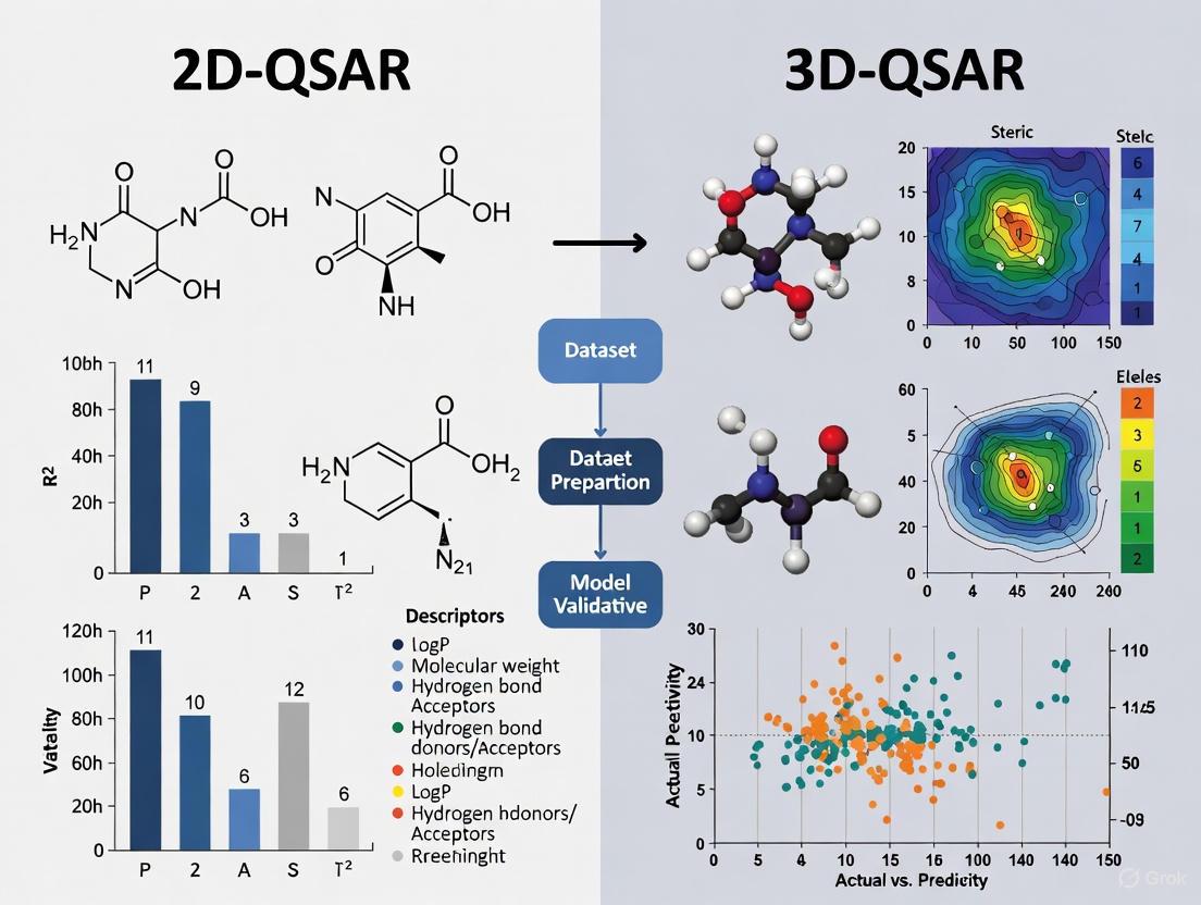
The 3D-QSAR contour maps provide visual guidance for rational drug design, indicating spatial regions where specific molecular modifications would enhance or diminish biological activity [14]. These maps translate the raw data of a 3D-QSAR model into an intuitive 'activity atlas' for medicinal chemists, showing where adding bulky groups increases (green contours) or decreases (yellow contours) activity, and which regions benefit from electronegative (red) or electropositive (blue) groups [14].

Diagram 2: Comparative analysis of 2D and 3D-QSAR approaches showing strengths, limitations, and research applications in glioblastoma drug discovery.

The comparative analysis of 2D and 3D-QSAR approaches for glioblastoma compound research demonstrates that each method offers distinct advantages depending on the research context. 2D-QSAR provides computationally efficient models with straightforward interpretation of key molecular descriptors, making it valuable for initial compound screening and prioritization. Meanwhile, 3D-QSAR approaches, particularly CoMSIA methods, deliver superior predictive performance and provide visual guidance for rational drug design through contour maps that highlight critical molecular regions for activity optimization.

The integration of both approaches—combining the descriptor-based insights from 2D-QSAR with the spatial field information from 3D-QSAR—proved particularly powerful in the design of novel dihydropteridone derivatives with enhanced anti-glioma activity [8]. This synergistic application offers a robust framework for advancing glioblastoma drug discovery, potentially contributing to the development of more effective chemotherapeutic agents for this challenging malignancy. As computational methods continue to evolve, the combination of these QSAR strategies with other in silico approaches such as molecular docking and dynamics simulations presents a promising path forward for addressing the critical unmet need in glioblastoma therapy.

The Importance of Comparing 2D and 3D-QSAR in Oncology Drug Discovery

In the relentless pursuit of effective oncology therapeutics, particularly for complex malignancies like glioblastoma (GBM), quantitative structure-activity relationship (QSAR) modeling has emerged as an indispensable tool for accelerating drug discovery. These computational approaches efficiently correlate the structural features of compounds with their biological activity, enabling the prediction of compound efficacy before costly synthesis and experimental testing. However, a critical question persists in modern cheminformatics: which QSAR paradigm—traditional 2D-QSAR or spatially informed 3D-QSAR—offers superior performance for specific oncology applications? The strategic comparison of these methodologies is not merely an academic exercise but a practical necessity for optimizing resource allocation, improving predictive accuracy, and ultimately designing more effective cancer treatments. This guide provides an objective, data-driven comparison of 2D and 3D-QSAR performance, leveraging experimental data from recent glioblastoma research to inform selection criteria for drug development professionals.

Theoretical Foundations and Methodological Divergence

2D-QSAR: Descriptor-Driven Predictive Modeling

2D-QSAR relies on molecular descriptors derived from the two-dimensional chemical structure, encompassing physicochemical properties (e.g., logP, molecular weight), electronic features, and topological indices [17]. These descriptors are numerically encoded and correlated with biological activity using statistical or machine learning methods such as Multiple Linear Regression (MLR), Partial Least Squares (PLS), or more advanced algorithms like Support Vector Machines (SVM) and Random Forests (RF) [18] [19]. The primary strength of 2D-QSAR lies in its computational efficiency and its ability to handle large chemical datasets without requiring molecular alignment or conformational analysis.

3D-QSAR: Incorporating Spatial Molecular Fields

In contrast, 3D-QSAR methodologies, such as Comparative Molecular Field Analysis (CoMFA) and Comparative Molecular Similarity Indices Analysis (CoMSIA), consider the three-dimensional arrangement of molecules [8] [20]. These techniques calculate steric (shape), electrostatic, hydrophobic, and hydrogen-bonding fields around a set of aligned molecules. The core hypothesis is that a molecule's biological activity is dependent on its interaction with a receptor, which is profoundly influenced by these spatial characteristics [21]. While more computationally intensive and sensitive to molecular alignment, 3D-QSAR provides直观的 visual contour maps that offer direct structural guidance for molecular optimization.

Table 1: Fundamental Characteristics of 2D and 3D-QSAR Approaches

Feature	2D-QSAR	3D-QSAR
Molecular Representation	Topological descriptors, physicochemical properties	3D steric, electrostatic, and hydrophobic fields
Key Descriptors	Molecular weight, logP, HOMO/LUMO energies, topological indices [17]	Field values at grid points surrounding aligned molecules
Common Algorithms	MLR, PLS, SVM, Random Forests [18] [19]	PLS, CoMFA, CoMSIA [8] [20]
Alignment Dependent	No	Yes
Primary Output	Mathematical equation correlating descriptors to activity	3D contour maps indicating favorable/unfavorable regions for substitution

Performance Benchmarking: Quantitative Evidence from Glioblastoma Research

Direct comparative studies and individual case applications in oncology provide compelling data on the relative performance of 2D and 3D-QSAR models.

A Direct Comparative Study on Dihydropteridone Derivatives

A 2023 study investigating dihydropteridone derivatives as PLK1 inhibitors for glioblastoma treatment offers a direct, quantitative comparison. The researchers constructed multiple QSAR models and evaluated their performance using standard statistical metrics [8].

Table 2: Performance Metrics of QSAR Models for Dihydropteridone Derivatives [8]

Model Type	Specific Method	R² (Training)	Q² (Cross-Validation)	Standard Error of Estimate (SEE)
2D-QSAR (Linear)	Heuristic Method (HM)	0.6682	0.5669	-
2D-QSAR (Non-Linear)	Gene Expression Programming (GEP)	0.79	0.76	-
3D-QSAR	CoMSIA	0.928	0.628	0.160

The data demonstrates a clear performance hierarchy. The 3D-QSAR (CoMSIA) model achieved a superior fit for the training data, as indicated by the highest R² value (0.928), signifying it explains over 92% of the variance in biological activity. It also exhibited a strong cross-validated correlation coefficient (Q²=0.628) and a low standard error of estimate [8]. The study authors concluded that "the 3D paradigm evinced an exemplary fit," outperforming the non-linear 2D model, while the linear 2D model showed suboptimal efficacy [8].

Performance in Other Oncological Targets

Evidence from other cancer types reinforces this trend. A study on EGFR inhibitors found that a 2D-QSAR model using SVM excelled in binary classification (predicting inhibitor vs. non-inhibitor) with an accuracy exceeding 97% [19]. However, for predicting the continuous value of inhibitory activity (IC50), the 3D-QSAR (Topomer CoMFA) model provided a high non-cross-validated correlation coefficient (r² = 0.888), demonstrating its strength in quantifying potency [19]. This highlights a key differentiator: 2D-QSAR can be highly effective for classification tasks, while 3D-QSAR often excels at predicting precise activity levels, which is critical for lead optimization.

Conversely, a study on histamine H3 receptor antagonists found that 2D methods (MLR and ANN) performed equally well or even better than the 3D-HASL method in predicting receptor binding affinities [18]. This indicates that the superiority of either approach can be context-dependent, influenced by the specific target and chemical series under investigation.

Experimental Protocols for QSAR Model Construction

The construction of robust QSAR models follows a systematic workflow. The general process and methodological differences between 2D and 3D approaches are outlined below.

Detailed Methodological Breakdown

Step 1: Dataset Curation and Preparation A series of compounds with known biological activities (e.g., IC50 or Ki values) is collected. For the dihydropteridone study, 34 compounds were used [8]. The dataset is typically partitioned into a training set (~75-80%) for model building and a test set (~20-25%) for external validation [8] [19].

Step 2: Molecular Structure Optimization and Alignment

• 2D-QSAR: Molecular structures are sketched and energetically minimized using molecular mechanics force fields (e.g., MM+). Further optimization may employ semi-empirical methods (AM1 or PM3) [8].
• 3D-QSAR: This critical additional step involves superimposing (aligning) all molecules based on a common scaffold or pharmacophore. The most active molecule is often used as a template for alignment [20].

Step 3: Descriptor Calculation and Field Generation

• 2D-QSAR: Software like CODESSA or DRAGON calculates thousands of molecular descriptors encompassing constitutional, topological, geometrical, and quantum-chemical features [8] [17]. Feature selection algorithms (e.g., CfsSubsetEval with Greedy Stepwise) are then used to identify the most relevant descriptors and avoid overfitting [19].
• 3D-QSAR: Programs like SYBYL compute steric (Lennard-Jones) and electrostatic (Coulombic) interaction energies at thousands of grid points surrounding the aligned molecules. CoMSIA can additionally calculate hydrophobic and hydrogen-bonding fields [20].

Step 4: Model Construction and Validation

• Partial Least Squares (PLS) regression is the standard algorithm for 3D-QSAR due to the high collinearity of field descriptors [8] [20]. For 2D-QSAR, PLS, MLR, and machine learning methods like SVM are common [19].
• Models are rigorously validated. Key metrics include:
  • R²: Coefficient of determination for the training set.
  • Q² (or q²): Cross-validated correlation coefficient (e.g., from Leave-One-Out), assessing predictive reliability. A Q² > 0.5 is generally considered acceptable [19].
  • External Validation: Predictive power on the independent test set, confirming model robustness [10].

Application in Glioblastoma Research: A Case Study

The integrated application of 2D and 3D-QSAR is powerfully illustrated in the discovery of novel dihydropteridone derivatives for glioblastoma.

The study began by developing both 2D and 3D models, confirming the higher statistical performance of the 3D-CoMSIA model [8]. The 2D model identified the most significant molecular descriptor as "Min exchange energy for a C-N bond" (MECN), providing an initial structural insight. However, the 3D-CoMSIA model generated visual contour maps that graphically illustrated regions around the molecular scaffold where specific chemical modifications would enhance or diminish activity [8].

By combining the quantitative descriptor from the 2D model with the qualitative, spatial guidance from the 3D contour maps, the researchers designed 200 novel compounds in silico. They predicted their activity and selected the most promising candidate, compound 21E.153, for synthesis and experimental testing. This compound demonstrated outstanding antitumor properties and strong binding affinity in molecular docking studies, validating the synergistic power of the combined QSAR approach [8].

This workflow, integrating the broader screening capability of 2D-QSAR with the precise optimization guidance of 3D-QSAR, is a hallmark of modern computer-aided drug design for challenging oncology targets [10] [22].

The Scientist's Toolkit: Essential Research Reagents and Solutions

Table 3: Key Software and Tools for QSAR Modeling in Oncology Drug Discovery

Tool Name	Type	Primary Function in QSAR	Relevance
CODESSA	Software	Calculates a wide range of 2D molecular descriptors [8].	Essential for generating input variables for 2D-QSAR models.
SYBYL	Software Suite	Provides a environment for molecular modeling, alignment, and performing 3D-QSAR (CoMFA, CoMSIA) [20] [19].	Industry-standard platform for constructing and visualizing 3D-QSAR models.
RDKit	Open-Source Cheminformatics	Calculates molecular descriptors and fingerprints; used for data preprocessing and model building, often within KNIME [10] [17].	A versatile and accessible tool for descriptor calculation and integration into data pipelines.
KNIME / scikit-learn	Data Analytics Platform / ML Library	Provides workflows (KNIME) and algorithms (scikit-learn) for data preparation, feature selection, and machine learning model construction [10] [17].	Crucial for building, validating, and deploying modern 2D-QSAR models using ML algorithms.

The empirical evidence from oncology drug discovery clearly indicates that 3D-QSAR methodologies often provide a more accurate and visually interpretable model for optimizing compound potency, as demonstrated by superior R² and Q² values in direct comparisons [8]. However, 2D-QSAR remains a highly valuable, computationally efficient approach for rapid virtual screening of large compound libraries and for classification tasks [18] [19].

For researchers and drug development professionals, the following strategic recommendations are proposed:

• Use 2D-QSAR for: Initial screening of large virtual libraries, identifying key physicochemical properties governing activity, and classification problems (e.g., active/inactive prediction).
• Use 3D-QSAR for: Lead optimization stages where understanding the spatial requirements of the target binding site is crucial, and for generating visual guides for medicinal chemists.
• Adopt an Integrated Approach: The most effective strategy leverages the strengths of both. Use 2D-QSAR to narrow the field of candidates and then apply 3D-QSAR to refine and optimize the most promising leads, as exemplified in the glioblastoma case study [8].

Ultimately, the choice between 2D and 3D-QSAR is not a binary one. A synergistic workflow that integrates both approaches, alongside other computational techniques like molecular docking and ADMET prediction, creates a powerful engine for driving innovation in oncology therapeutics, offering new hope for treating devastating diseases like glioblastoma [10] [22].

Implementing QSAR Models: Step-by-Step Methods for Glioblastoma Compound Analysis

Data Collection and Preprocessing for 2D and 3D-QSAR Studies

Quantitative Structure-Activity Relationship (QSAR) modeling represents a fundamental methodology in modern computational drug discovery, establishing mathematical relationships between chemical structures and their biological activities. In the challenging field of glioblastoma (GBM) research, where therapeutic options remain limited, QSAR approaches provide valuable tools for rational drug design. GBM, as the most aggressive and treatment-resistant variant of brain tumors, presents formidable therapeutic challenges due to its high complexity, protective blood-brain barrier, and rapid progression dynamics [22]. The resistance of GBM to conventional treatments stems from its internal subpopulations of stem cells and highly mutated genome, complicating treatment strategies and creating an urgent need for novel therapeutic approaches [5].

QSAR methodologies have evolved significantly from classical approaches to modern artificial intelligence-integrated frameworks, offering powerful means to accelerate the discovery of potential GBM therapeutics. These computational approaches significantly accelerate the preclinical stage of drug discovery by reducing costs, minimizing attrition, and expediting the identification of viable candidates [17]. For glioblastoma research specifically, QSAR models have been successfully applied to various promising targets, including Polo-like kinase 1 (PLK1) inhibitors like dihydropteridone derivatives and Focal Adhesion Kinase (FAK) inhibitors, both representing innovative strategies in GBM treatment [4] [5]. This guide systematically compares the data collection and preprocessing requirements for 2D and 3D-QSAR studies, providing researchers with practical protocols and experimental frameworks tailored to glioblastoma compound research.

Fundamental QSAR Concepts and Definitions

At its core, QSAR is defined as a methodology to associate the chemical structure of a molecule with its biochemical, physical, pharmaceutical, or biological effects [23]. The fundamental equation can be summarized as: Biological activity = f(physicochemical parameters) [23]. This mathematical framework enables researchers to predict compound behavior without extensive laboratory experimentation, creating significant efficiencies in the drug discovery pipeline.

QSAR techniques are systematically classified based on the dimensionality of molecular descriptors used in model construction. Two-dimensional (2D) QSAR focuses on molecular descriptors derived from the compound's topological structure without considering spatial orientation, while three-dimensional (3D) QSAR incorporates the molecule's spatial configuration and interaction potentials into the modeling approach [24]. The progression from 2D to 3D-QSAR represents an evolution from considering molecules as flat structural diagrams to treating them as three-dimensional objects with specific shapes and interaction fields [14].

The motivation behind developing QSAR models in glioblastoma research encompasses several critical objectives: predicting biological activity of novel compounds, rationalizing mechanisms of action within chemical series, reducing compound development expenses, minimizing animal testing requirements, and advancing greener chemistry approaches by eliminating unlikely leads early in the discovery process [23]. For GBM specifically, where blood-brain barrier penetration represents a critical additional hurdle, QSAR models can incorporate parameters predicting this crucial property alongside anti-tumor efficacy [22].

Data Collection Protocols for QSAR Modeling

Compound Selection and Activity Data Acquisition

The foundation of any robust QSAR model lies in the quality and relevance of the underlying dataset. For glioblastoma-focused studies, researchers typically assemble compounds with experimentally determined activity values against specific GBM-related targets or cell lines. The integrity of this dataset is paramount, requiring selection of molecules that are structurally related to ensure coherent modeling, yet sufficiently diverse to capture meaningful structure-activity relationships [14]. All activity data must be acquired under uniform experimental conditions, as variability in assay protocols introduces unwanted noise and systemic bias that compromises predictive value [14].

Specific protocols for GBM-targeted datasets have been demonstrated in recent studies. For FAK inhibitors targeting glioblastoma, researchers retrieved molecular structures and corresponding inhibitory activity (expressed as half-maximal inhibitory concentration IC50) from the CHEMBL database (CHEMBL2695), initially comprising 4730 entries [5]. The base-10 logarithm of IC50 (represented as -logIC50, denoted as pIC50) typically serves as the dependent variable rather than raw IC50 values. For compounds displaying varying IC50 values within a narrow range (10 μM), the average is calculated as the final IC50 value to ensure data consistency [5]. Similarly, for PLK1 inhibitors like dihydropteridone derivatives, studies have obtained structures and corresponding activity values from published research, with one study utilizing 34 compounds for initial model development [4].

Table 1: Standardized Activity Data Format for QSAR Modeling

Field Name	Data Type	Description	Example Value
Compound ID	String	Unique identifier	CMPD-001
SMILES	String	Structural representation	C1=CC(=CC=C1F)
IC50 (nM)	Numeric	Half-maximal inhibitory concentration	125.0
pIC50	Numeric	-log10(IC50)	6.90
Target	String	Biological target	PLK1 kinase
Assay Type	String	Experimental method	Cell-based U87-MG
Reference	String	Data source	CHEMBL2695

Dataset Partitioning Strategies

To mitigate overfitting risks and ensure model generalizability, randomized partitioning of compounds is essential. Studies typically employ a ratio of approximately 1:3, allocating a smaller subset (e.g., 8 compounds from a set of 34) to the test set and the majority (e.g., 26 compounds) to the training set [4]. The training set serves to establish and refine the model, encompassing construction, calibration, and identification of key variables and algorithms. Meanwhile, the test set provides unbiased assessment without parameter modification, with decisions regarding algorithm adjustments or model retraining contingent upon evaluating the overall model fit [4].

For larger datasets, such as those comprising 1280 FAK inhibitors, researchers may implement more sophisticated splitting strategies, including an 80:20 ratio for training and independent test sets, with ten-fold cross-validation during model training to mitigate the impact of random data partitioning [5]. Optimization techniques such as hyperparameter tuning using grid search methodology further enhance model performance, with optimal parameters determined specifically for each algorithm employed [5].

Preprocessing Methodologies for 2D-QSAR

Molecular Structure Optimization and 2D Descriptor Calculation

The performance of 2D-QSAR models relies heavily on appropriate selection of molecular descriptors, necessitating careful structural optimization of investigated compounds. In standard protocols, the chemical structure is initially sketched using ChemDraw and subsequently optimized using HyperChem [4]. The optimization process typically employs molecular mechanics field (MM+) for initial optimization, followed by selection of the AM1 or PM3 model based on the presence or absence of S and P atoms. The structure is cyclically optimized using the Polak-Ribiere method until the root mean square gradient reaches a threshold of 0.01 [4].

Following structural optimization, computational programs like CODESSA calculate molecular descriptors encompassing quantum chemistry, structure, topology, geometry, and electrostatic properties [4]. These 2D descriptors include pure topological descriptors, connectivity indices, walk and path counts, information indices, and 2D-autocorrelations [24]. Alternatively, researchers may utilize PaDEL-Descriptor, an open source software capable of generating 1875 descriptors including 1D, 2D, and 3D types, along with 12 types of fingerprints [24]. Dragon represents another option, capable of generating more than 4000 descriptors for a single molecule, with a web-based version available for limited use [24].

Descriptor Selection and Linear Model Construction

In constructing linear 2D-QSAR models, the Heuristic Method (HM) is frequently employed to extract all molecular descriptors, followed by feature selection to determine the optimal number of descriptors that effectively represent chemical structure while excluding descriptors with minimal impact [4]. Objective measures, such as the F-test, R², R²CV, and t-test, evaluate correlation coefficients between parameters. Additional descriptors are iteratively added until further inclusion has negligible influence on results [4]. Through this procedure, linear models typically incorporate multiple descriptors, with studies identifying "Min exchange energy for a C-N bond" (MECN) as particularly significant for dihydropteridone derivatives against GBM [4].

For nonlinear 2D-QSAR modeling, Gene Expression Programming (GEP) has emerged as a powerful technique rooted in programming and algorithms [4]. Unlike coding numbers or analyzing trees, GEP utilizes linear chromosomes as candidates, with coding of constant-length linear symbols and derivation of individual phenotypes similar to coding codes and expression trees [4]. The candidate chromosomes are generated from the feature set and the end set, then encoded into an expression tree (ET) format to calculate the equation, with fitness functions applied to a random number of chromosomes until termination conditions are met [4].

Table 2: Performance Comparison of 2D-QSAR Modeling Approaches for Glioblastoma Compounds

Model Type	Statistical Metric	Performance Value	Dataset Characteristics	Application Example
Heuristic Method (Linear)	R²	0.6682	34 dihydropteridone derivatives	PLK1 inhibitors [4]
	R²cv	0.5669
	Residual sum of squares (S²)	0.0199
Gene Expression Programming (Nonlinear)	Training set R²	0.79	34 dihydropteridone derivatives	PLK1 inhibitors [4]
	Validation set R²	0.76
LightGBM (Machine Learning)	R²	0.892	1280 FAK inhibitors	FAK inhibitors for GBM [5]
	MAE	0.331
	RMSE	0.467

Preprocessing Methodologies for 3D-QSAR

Molecular Modeling and Conformational Analysis

Three-dimensional QSAR begins with generating 3D molecular structures by converting 2D representations into three-dimensional coordinates using cheminformatics tools like RDKit or Sybyl [14]. These initial 3D structures undergo geometry optimization using molecular mechanics such as the universal force field (UFF) or, for higher accuracy, quantum mechanical methods [14]. Optimization ensures each molecule adopts a realistic, low-energy conformation, which critically influences subsequent alignment and descriptor calculation steps.

The selected conformation must reflect the putative bioactive orientation, with prioritization of structural accuracy at this stage being essential for model quality. Since small molecules often exhibit conformational flexibility, some advanced 3D-QSAR approaches incorporate multiple low-energy conformations to account for this variability, though this increases computational complexity significantly [24]. For glioblastoma-targeted compounds, particular attention must be paid to conformations that potentially facilitate blood-brain barrier penetration alongside target binding.

Molecular Alignment Techniques

Molecular alignment constitutes one of the most critical and technically demanding steps in 3D-QSAR, with the objective of superimposing all molecules within a shared 3D reference frame that reflects their putative bioactive conformations [14]. This alignment assumes that all compounds share a similar binding mode and can be accomplished through manual approaches or algorithmic methods.

Common alignment strategies include Bemis-Murcko scaffolding, which derives scaffolds by removing side chains and retaining only ring systems and linkers, and maximum common substructure (MCS), which identifies the largest shared substructure among a set of molecules [14]. Tools like RDKit's AllChem.ConstrainedEmbed() can generate 3D conformations that match scaffold atoms to a reference, ensuring accurate alignment. A poor alignment undermines the entire modeling process by introducing inconsistencies in descriptor calculations, which is why some modern methods aim to bypass alignment altogether, though traditional approaches such as Comparative Molecular Field Analysis (CoMFA) remain alignment-dependent [14].

Diagram 1: 3D-QSAR Preprocessing Workflow. This workflow illustrates the sequential steps in 3D-QSAR preprocessing, from initial 2D structures through model building and prediction.

3D Molecular Descriptor Computation

Following alignment, researchers compute 3D molecular descriptors that numerically represent steric and electrostatic environments of each molecule. The classic Comparative Molecular Field Analysis (CoMFA) method uses a lattice of grid points surrounding the molecules, where a probe atom measures interaction energies at each point - typically steric (van der Waals) and electrostatic (Coulomb) interaction energies [14]. This approach essentially maps how a tiny test probe "feels" the presence of the molecule at various locations, detecting bulky groups or attractive positive charges [14]. The collection of all field values forms a fingerprint-like descriptor for the molecule's 3D shape and electrostatic profile.

Comparative Molecular Similarity Indices Analysis (CoMSIA) extends this approach by using Gaussian-type functions to evaluate steric, electrostatic, hydrophobic, and hydrogen-bonding fields, which smooth out abrupt field changes and enhance interpretability, especially across structurally diverse compounds [14]. While CoMFA is highly sensitive to alignment quality, requiring precise spatial congruence across molecules, CoMSIA offers more tolerance to minor misalignments, thereby expanding applicability to datasets with broader chemical diversity [14].

Model Building and Validation in 3D-QSAR

With 3D descriptors calculated for a series of molecules and their known biological activities, the next step establishes a mathematical relationship linking 3D descriptor values to biological activity. Statistical regression techniques like partial least squares (PLS) regression are standard in CoMFA and many 3D-QSAR studies, as PLS can handle the large number of highly correlated descriptors by projecting them to a smaller set of latent variables [14]. The outcome is a mathematical model capable of predicting biological activity from 3D field data.

Model validation represents a crucial step, typically employing cross-validation techniques such as leave-one-out (LOO), where each compound is sequentially excluded from the training set and predicted by a model built from the remaining data [14]. Researchers quantify model performance using statistical metrics: Q² for cross-validated predictivity and R² for goodness-of-fit. A robust model should exhibit high values for both metrics, indicating capture of meaningful biological trends without overfitting. For glioblastoma-focused 3D-QSAR, exemplary models have demonstrated exemplary fit with formidable Q² (0.628) and R² (0.928) values, complemented by impressive F-value (12.194) and minimized standard error of estimate (SEE) at 0.160 [4].

Table 3: Performance Metrics for 3D-QSAR Models in Glioblastoma Research

Model Type	Statistical Metric	Performance Value	Dataset	Key Advantage
CoMFA	Q²	0.528	22 FAK inhibitors	Steric/electrostatic field analysis [5]
	R²pred	0.7557
CoMSIA	Q²	0.757	22 FAK inhibitors	Additional hydrophobic/H-bond fields [5]
	R²pred	0.8362
Advanced 3D-QSAR	Q²	0.628	34 dihydropteridone derivatives	Excellent fit statistics [4]
	R²	0.928
	F-value	12.194
	SEE	0.160

Comparative Performance Analysis for Glioblastoma Applications

Predictive Accuracy and Model Robustness

Direct comparison of 2D and 3D-QSAR approaches reveals distinct performance characteristics relevant to glioblastoma drug discovery. Empirical modeling outcomes consistently underscore the preeminence of 3D-QSAR models, followed by nonlinear 2D models, while linear 2D approaches often manifest suboptimal efficacy [4]. Specifically, for dihydropteridone derivatives targeting PLK1 in GBM, the 3D-QSAR paradigm demonstrated exemplary fit characterized by formidable Q² (0.628) and R² (0.928) values, complemented by an impressive F-value (12.194) and minimized standard error of estimate (SEE) at 0.160 [4]. In contrast, the heuristic 2D linear model achieved an R² of 0.6682 with R²cv of 0.5669, while the GEP nonlinear 2D model showed improved performance with coefficients of determination for training and validation sets at 0.79 and 0.76, respectively [4].

For FAK inhibitors targeting glioblastoma, machine learning-enhanced 2D approaches have demonstrated strong predictive capability, with models based on 1280 FAK inhibitors achieving R² of 0.892, MAE of 0.331, and RMSE of 0.467 using combined CDK, CDK extended fingerprints, and substructure fingerprint counts [5]. Another model based on IC50 data from 2608 compounds tested on U87-MG cells achieved an R² of 0.789, MAE of 0.395, and RMSE of 0.536 [5]. These results suggest that while 3D-QSAR generally offers superior performance for congeneric series, advanced 2D approaches with large datasets can achieve competitive predictive accuracy.

Interpretability and Design Guidance

A critical distinction between 2D and 3D-QSAR lies in their interpretability and capacity to guide molecular design. 3D-QSAR models excel in providing visual guidance through contour maps that identify spatial regions where specific molecular features enhance or diminish activity [14]. For example, steric contour maps show where adding bulky groups is favorable (green regions) or should be avoided (yellow regions), while electrostatic maps indicate regions that benefit from electronegative (red) or electropositive (blue) groups [14]. These visual cues directly inform rational chemical modifications by highlighting structural regions amenable to optimization.

In contrast, 2D-QSAR models identify significant molecular descriptors that influence activity but provide less direct spatial guidance for molecular design. The most significant molecular descriptors in 2D models, such as "Min exchange energy for a C-N bond" (MECN) identified for dihydropteridone derivatives, offer important insights into electronic properties affecting activity but lack the three-dimensional context of contour maps [4]. However, by combining key 2D descriptors with hydrophobic field information, researchers can generate valuable suggestions for novel drug design, as demonstrated by the identification of compound 21E.153, a novel dihydropteridone derivative with outstanding antitumor properties and docking capabilities [4].

Diagram 2: QSAR Approach Selection Guide. This decision diagram illustrates key factors influencing the choice between 2D and 3D-QSAR approaches for glioblastoma compound research.

Software Solutions for QSAR Modeling

The successful implementation of QSAR studies requires specialized software tools for descriptor calculation, model building, and validation. Multiple commercial and open-source options exist, each with particular strengths for glioblastoma research applications. For 2D-QSAR, PaDEL-Descriptor represents a popular open-source choice, capable of generating 1875 descriptors including 1D, 2D, and 3D types alongside 12 fingerprint types [24]. Dragon offers even more extensive descriptor calculation, generating over 4000 descriptors for a single molecule, with a freely available web-based version for limited use [24].

For 3D-QSAR studies, specialized software includes Pentacle from Molecular Discovery, which implements the GRIND approach, and Schrodinger's AutoQSAR for automated 3D-QSAR modeling [24]. Comparative Molecular Field Analysis (CoMFA) and Comparative Molecular Similarity Indices Analysis (CoMSIA) remain cornerstone methodologies, available in commercial packages like Sybyl and open-source alternatives [24] [14]. Workflow automation tools such as Taverna, Pipeline Pilot, Galaxy, and KNIME provide platforms for developing complete QSAR workflows, integrating data retrieval, descriptor calculation, model building, and validation into streamlined processes [24].

Table 4: Essential Software Tools for QSAR Studies in Glioblastoma Research

Software Tool	License Type	Primary Function	Application in GBM Research
PaDEL-Descriptor	Free	Molecular descriptor calculation	Generate 2D descriptors for blood-brain barrier penetration prediction
Dragon	Commercial/Free limited	Molecular descriptor calculation	Comprehensive descriptor calculation for machine learning QSAR
AutoQSAR	Commercial	Automated 3D-QSAR model creation	Rapid screening of GBM compound libraries
CODESSA	Commercial	QSAR modeling and descriptor calculation	Heuristic method implementation for PLK1 inhibitors
KNIME	Free	Workflow automation	Building complete QSAR pipelines for FAK inhibitors
RDKit	Free	Cheminformatics and 3D alignment	Molecular conformation generation and scaffold-based alignment
QSARpro	Commercial	QSAR modeling and activity prediction	Toxicity prediction for GBM drug candidates

Experimental Protocols for Specific GBM Targets

For researchers targeting specific glioblastoma pathways, tailored QSAR protocols have demonstrated particular success. For PLK1 inhibitors like dihydropteridone derivatives, studies have established optimized protocols involving the Heuristic Method for linear 2D-QSAR with six descriptors, GEP for nonlinear modeling, and CoMSIA for 3D-QSAR with integrated electrostatic, steric, hydrophobic, and hydrogen-bonding fields [4]. The most significant molecular descriptor identified (MECN - Min exchange energy for a C-N bond) combined with hydrophobic field information provides specific design guidance for novel compounds [4].

For FAK inhibitors targeting glioblastoma, machine learning-enhanced protocols utilizing LightGBM, Random Forest, and XGBoost algorithms with molecular fingerprints have proven effective for large-scale virtual screening [5]. These approaches leverage extensive datasets (1280+ compounds) from CHEMBL, employing CDK fingerprints, CDK extended fingerprints, substructure fingerprints, and substructure fingerprint counts as molecular descriptors [5]. Subsequent ADMET analysis and molecular dynamics simulations further refine candidate selection, providing a comprehensive framework for FAK inhibitor development specific to GBM therapeutic needs [5].

The comparative analysis of data collection and preprocessing methodologies for 2D and 3D-QSAR studies reveals a complementary relationship between these approaches in glioblastoma drug discovery. While 3D-QSAR generally offers superior predictive accuracy and provides visual guidance through contour maps, it demands careful conformational analysis and alignment, making it particularly suitable for congeneric series with established binding modes. Conversely, 2D-QSAR approaches, especially when enhanced with machine learning algorithms, demonstrate robust performance with large, diverse datasets and offer implementation advantages through simpler preprocessing requirements.

For glioblastoma researchers, the selection between 2D and 3D-QSAR should be guided by specific research contexts: dataset characteristics, computational resources, target knowledge, and desired output. The integration of both approaches, leveraging 2D-QSAR for initial large-scale screening and 3D-QSAR for detailed optimization of promising leads, represents a powerful strategy for advancing GBM therapeutics. Furthermore, the emerging integration of AI methodologies with both 2D and 3D-QSAR promises enhanced predictive capability and efficiency, potentially accelerating the development of critically needed novel treatments for this challenging disease. As QSAR methodologies continue evolving, their application in glioblastoma research will undoubtedly expand, offering increasingly sophisticated tools for addressing one of oncology's most formidable challenges.

Quantitative Structure-Activity Relationship (QSAR) modeling represents a cornerstone of computer-aided drug design, enabling researchers to predict the biological activity of compounds through mathematical relationships derived from their chemical structures. In the context of glioblastoma research—an area with urgent unmet therapeutic needs—QSAR methodologies provide valuable tools for accelerating the identification of novel chemotherapeutic agents. While 3D-QSAR approaches offer insights into spatial molecular interactions, 2D-QSAR remains widely utilized for its computational efficiency, interpretability, and effectiveness, particularly in early-stage drug discovery campaigns [8] [25]. The robustness of a 2D-QSAR model hinges critically on two fundamental components: the judicious selection of molecular descriptors that encode crucial structural information, and the implementation of appropriate algorithms that can accurately capture the relationship between these descriptors and biological activity [26] [25].

The evolution of QSAR from classical statistical methods to modern machine learning-based approaches has significantly expanded its predictive capabilities. Traditional methods like Multiple Linear Regression (MLR) and Partial Least Squares (PLS) remain valued for their interpretability, while contemporary machine learning algorithms can capture complex, non-linear relationships in high-dimensional chemical data [26] [18]. This comparative guide examines the construction of robust 2D-QSAR models, with particular emphasis on descriptor selection strategies and algorithm implementation, while objectively evaluating its performance relative to 3D-QSAR approaches in the context of glioblastoma therapeutic development.

Theoretical Foundations of 2D-QSAR

Molecular Descriptors: Encoding Chemical Information

Molecular descriptors are numerical representations of a compound's structural and physicochemical properties that serve as the independent variables in QSAR models. These descriptors are broadly classified based on the dimensions of chemical information they encode. 1D descriptors represent bulk properties like molecular weight and atom count; 2D descriptors capture topological features derived from molecular connectivity; while 3D descriptors quantify spatial characteristics such as shape and electrostatic potential [26]. For 2D-QSAR, topological descriptors are particularly relevant as they can be calculated directly from molecular structure without requiring conformational analysis or alignment [25].

The appropriate selection and interpretation of these descriptors is paramount for developing predictive, robust QSAR models. As noted in studies of dihydropteridone derivatives as PLK1 inhibitors for glioblastoma, the most significant molecular descriptor in a 2D model was identified as "Min exchange energy for a C-N bond" (MECN), which contributed substantially to predicting anticancer activity [8]. Modern descriptor calculation tools like PaDEL software, DRAGON, and RDKit can generate thousands of molecular descriptors encompassing quantum chemical, structural, topological, geometry, and electrostatic properties [26] [5]. To mitigate overfitting and enhance model interpretability, dimensionality reduction techniques such as Principal Component Analysis (PCA), Recursive Feature Elimination (RFE), and LASSO (Least Absolute Shrinkage and Selection Operator) are routinely employed to identify the most relevant descriptor subsets [26].

Algorithm Selection: From Classical Statistics to Machine Learning

The algorithmic framework used to correlate molecular descriptors with biological activity determines the model's capacity to capture underlying structure-activity relationships. Classical statistical methods including Multiple Linear Regression (MLR), Partial Least Squares (PLS), and Principal Component Regression (PCR) are esteemed for their simplicity, speed, and explanatory power, particularly in regulatory settings where interpretability is prioritized [26] [18]. These approaches perform effectively when a reasonably small number of variables exhibit linear relationships with the biological response, and they form the foundation of many published QSAR studies on anticancer agents [25] [18].

With advances in computational power and algorithm development, machine learning approaches have substantially expanded the capabilities of QSAR modeling. Algorithms such as Random Forests (RF), Support Vector Machines (SVM), k-Nearest Neighbors (kNN), and gradient boosting methods like LightGBM and XGBoost can effectively capture non-linear relationships without prior assumptions about data distribution [26] [5]. For instance, in a study focused on designing FAK inhibitors for glioblastoma, the LightGBM algorithm was prioritized due to its advantages as an ensemble learning method over conventional approaches, resulting in models with R² values of 0.892 using protein-level IC₅₀ data [5]. The increasing integration of artificial intelligence, particularly deep learning architectures such as Graph Neural Networks (GNNs) and SMILES-based transformers, represents the cutting edge of QSAR methodology, enabling the automatic learning of molecular representations without manual descriptor engineering [27] [26].

Experimental Protocols for 2D-QSAR Model Development

Dataset Preparation and Chemical Space Representation

The initial critical step in QSAR modeling involves the curation of a high-quality dataset with reliable biological activity measurements. In glioblastoma research, this typically involves compounds screened against specific molecular targets like PLK1 or FAK, or cellular activity on glioblastoma cell lines such as U87-MG [8] [5]. The biological activity is preferably expressed as the half-maximal inhibitory concentration (IC₅₀), which is converted to pIC₅₀ (-logIC₅₀) for modeling purposes to normalize the distribution [5]. To ensure model generalizability, the chemical space should be adequately sampled, with compounds spanning a wide range of structural features and activity potencies. For example, in a FAK inhibitor study, the dataset comprised 1,280 compounds with pIC₅₀ values ranging from 4.00 to 10.00, predominantly between 5.00 and 9.50, providing sufficient diversity for model training [5].

The dataset must be partitioned into training and test sets, typically following an 80:20 ratio, with the training set used for model construction and parameter optimization, and the test set reserved for external validation [5]. Stratified sampling based on activity distribution ensures both sets represent similar chemical space. For the 2D-QSAR analysis of dihydropteridone derivatives, a random partitioning was applied to the set of 34 compounds at a ratio of 1:3, resulting in 8 compounds assigned to the test set and 26 compounds allocated to the training set [8]. Proper dataset division is crucial for developing models with true predictive power for novel compounds.

Molecular Descriptor Calculation and Feature Selection

Following dataset preparation, molecular structures undergo geometry optimization, typically employing molecular mechanics force fields (e.g., MM+) followed by semi-empirical methods (e.g., AM1 or PM3) until the root mean square gradient reaches a threshold such as 0.01 [8]. Subsequently, molecular descriptor calculation is performed using specialized software packages such as CODESSA, PaDEL, or RDKit, which generate numerical values representing diverse molecular properties including electronic, topological, geometrical, and constitutional characteristics [8] [5].

With hundreds to thousands of possible descriptors computable, feature selection becomes essential to avoid overfitting and identify the most chemically meaningful descriptors. As demonstrated in a SARS-CoV-2 Mpro inhibitor study, initially selected 2D descriptors were cross-correlated using a linear Pearson correlation matrix to reduce redundancy [28]. Genetic Algorithm (GA) coupled with Partial Least Squares or stepwise multiple regression methods are frequently employed for descriptor selection [18]. For the dihydropteridone derivatives, the Heuristic Method (HM) was used to extract all molecular descriptors followed by feature selection to determine the optimal number of descriptors that effectively represent the chemical structure while excluding descriptors with minimal impact [8]. Objective measures including the F-test, R², R² CV, and t-test provide statistical guidance for descriptor selection.

Model Training and Validation

The core modeling phase involves training algorithms to establish mathematical relationships between selected molecular descriptors and biological activity. For classical approaches like MLR, this entails deriving regression coefficients that minimize the difference between predicted and experimental activity values [18]. Machine learning methods require additional hyperparameter optimization, often implemented through grid search or Bayesian optimization, to enhance predictive performance [5]. In the FAK inhibitor study, hyperparameter tuning was employed, and ten-fold cross-validation was implemented during model training to mitigate the impact of random data partitioning [5].

Rigorous validation is imperative to ensure model reliability and prevent overfitting. Internal validation techniques include cross-validation (e.g., leave-one-out or leave-group-out) which yields metrics such as Q² (cross-validated R²) [18]. External validation using the held-out test set provides the most realistic assessment of predictive power. For the dihydropteridone derivatives, the HM linear model demonstrated a coefficient of determination (R²) of 0.6682, with an R² cv of 0.5669 and a residual sum of squares (S²) of 0.0199 [8]. Additional validation techniques include Y-randomization tests, which rule out chance correlations, and applicability domain analysis, which defines the chemical space where model predictions are reliable [29].

Figure 1: 2D-QSAR Model Development Workflow

Comparative Performance: 2D-QSAR vs. 3D-QSAR

Methodological Comparisons

2D- and 3D-QSAR approaches differ fundamentally in their theoretical foundations and information requirements. While 2D-QSAR utilizes molecular descriptors derived from topological structure, 3D-QSAR methods such as Comparative Molecular Field Analysis (CoMFA) and Comparative Molecular Similarity Index Analysis (CoMSIA) require spatially aligned molecular conformations and analyze steric and electrostatic fields surrounding the molecules [29] [28]. This distinction has significant practical implications for drug discovery workflows. 3D-QSAR models are highly sensitive to molecular alignment rules and conformational selection, requiring careful consideration of bioactive conformations [28]. In contrast, 2D-QSAR models bypass alignment requirements entirely, making them particularly valuable when the target protein structure is unknown or when dealing with structurally diverse compound sets [25].

The computational demands also differ substantially between approaches. 3D-QSAR typically requires more extensive computational resources for conformation generation, molecular alignment, and field calculation [28]. A study on SARS-CoV-2 Mpro inhibitors noted that building 3D-QSAR models is highly sensitive to conformation searching and molecular alignments, whereas 2D-QSAR models based on physicochemical descriptors and fingerprints offered a less computationally intensive alternative [28]. However, 3D-QSAR provides superior interpretability in terms of spatial molecular requirements for activity, as evidenced by contour maps that visually represent regions where specific chemical features enhance or diminish biological activity [8] [28].

Predictive Performance and Applications

Direct comparisons of predictive performance between 2D- and 3D-QSAR approaches reveal context-dependent advantages. In glioblastoma research focused on dihydropteridone derivatives, empirical modeling outcomes underscored the preeminence of the 3D-QSAR model, followed by a gene expression programming (GEP) nonlinear 2D model, while the heuristic method (HM) linear 2D model manifested suboptimal efficacy [8]. The 3D-QSAR paradigm demonstrated an exemplary fit, characterized by formidable Q² (0.628) and R² (0.928) values, complemented by an impressive F-value (12.194) and a minimized standard error of estimate (SEE) at 0.160 [8].

However, this performance hierarchy is not universal across all datasets and target systems. In a study of SARS-CoV-2 Mpro inhibitors, both 2D- and 3D-QSAR models showed comparable predictive accuracy, with the best 2D model (Morgan FP MLP) achieving an r² test set of 0.72, identical to the best 3D-QSAR model (MLP) [28]. Similarly, research on histamine H3 receptor antagonists found that simple traditional MLR approaches performed equally well compared to more advanced 3D-QSAR analyses like HASL [18]. These comparative results suggest that the optimal QSAR approach depends on factors including dataset size, structural diversity, and the specific modeling objectives.

Table 1: Performance Comparison of 2D- and 3D-QSAR Models Across Therapeutic Areas

Therapeutic Area	Target	2D-QSAR Performance	3D-QSAR Performance	Reference
Glioblastoma	PLK1 (Dihydropteridone derivatives)	GEP nonlinear: R² training=0.79, R² validation=0.76	CoMSIA: Q²=0.628, R²=0.928	[8]
SARS-CoV-2	Mpro inhibitors	MLP (Morgan FP): r² test=0.72	MLP: r² test=0.72	[28]
Histamine H3 Receptor	Arylbenzofuran antagonists	MLR/ANN: MAPE=2.9-3.6, SDEP=0.31-0.36	HASL: Inferior to 2D methods	[18]
Malaria	P. falciparum (Quinoline derivatives)	2D-QSAR: r² test=0.845	CoMSIA: r² test=0.876	[29]

Synergistic Integration in Drug Discovery

Rather than existing as mutually exclusive alternatives, 2D- and 3D-QSAR approaches often provide complementary insights when integrated into drug discovery pipelines. The strategic combination of both methodologies can leverage their respective strengths while mitigating their limitations [8] [29]. For instance, 2D-QSAR models can efficiently screen large chemical databases to identify promising scaffolds, while 3D-QSAR can provide detailed structural guidance for lead optimization [26] [28].

In glioblastoma drug discovery, this integrated approach was exemplified in the study of dihydropteridone derivatives, where researchers combined the most significant molecular descriptor from the 2D model (MECN) with hydrophobic field information from 3D analysis to generate suggestions for novel compounds [8]. This synergistic approach led to the identification of compound 21E.153, a novel dihydropteridone derivative which exhibited outstanding antitumor properties and docking capabilities [8]. Similarly, in malaria research, both 2D- and 3D-QSAR models were developed for quinoline derivatives, with the CoMSIA and 2D-QSAR models outperforming CoMFA in terms of predictive capacity [29]. The complementary nature of these approaches provides a more comprehensive foundation for rational drug design than either method alone.

Table 2: Strategic Applications of 2D- and 3D-QSAR in Drug Discovery Workflows

Research Stage	2D-QSAR Advantages	3D-QSAR Advantages
Virtual Screening	High throughput, no alignment needed, handles large diverse libraries	Incorporates spatial molecular fields, structure-based insights
Lead Optimization	Identifies key substituents and physicochemical properties	Provides 3D contour maps for structural modification guidance
Scaffold Hopping	Effective across diverse chemotypes using topological descriptors	Requires structural similarity for meaningful alignments
Interpretability	Clear descriptor-activity relationships for medicinal chemists	Visual representation of favorable/unfavorable interaction regions
Resource Requirements	Lower computational demands, faster model development	Higher computational costs for conformation search and alignment

Essential Research Reagents and Computational Tools

Successful implementation of 2D-QSAR modeling requires access to specialized software tools and computational resources that facilitate descriptor calculation, model building, and validation. The field has benefited from the development of both commercial and open-source platforms that streamline the QSAR workflow, making these methodologies accessible to researchers across academic and industrial settings [26] [25].

Table 3: Essential Research Reagent Solutions for 2D-QSAR Modeling

Tool Category	Specific Examples	Key Functionalities	Application Context
Descriptor Calculation	CODESSA, PaDEL, RDKit, DRAGON	Compute molecular descriptors from chemical structures	Generation of topological, electronic, and physicochemical descriptors [8] [5]
Cheminformatics	KNIME, Orange, DataWarrior	Data preprocessing, visualization, and analysis	Chemical space analysis, descriptor selection, and dataset curation [26] [5]
Machine Learning	scikit-learn, TensorFlow, PyTorch	Implementation of ML algorithms for QSAR	Model training with RF, SVM, GNN, and other algorithms [26] [5]
Molecular Modeling	HyperChem, ChemDraw, OpenBabel	Structure sketching and geometry optimization	Initial structure preparation and energy minimization [8]
Validation Tools	QSARINS, Build QSAR	Advanced model validation and applicability domain assessment	Internal and external validation, adherence to OECD principles [26]

The development of robust 2D-QSAR models represents a critical methodology in the computational arsenal for glioblastoma therapeutic development. While 3D-QSAR approaches provide valuable spatial insights for lead optimization, 2D-QSAR offers distinct advantages in computational efficiency, applicability to diverse chemical datasets, and effectiveness for virtual screening. The integration of machine learning algorithms has substantially enhanced the predictive power of 2D-QSAR models, enabling them to capture complex, non-linear structure-activity relationships that elude classical statistical methods [26] [5].

The comparative analysis presented in this guide demonstrates that the selection between 2D- and 3D-QSAR approaches should be guided by specific research objectives, dataset characteristics, and available computational resources. For glioblastoma research, where rapid identification of novel chemotherapeutic agents is urgently needed, 2D-QSAR provides an efficient screening tool that can prioritize compounds for subsequent experimental validation [8] [5]. The most effective drug discovery pipelines strategically combine both methodologies, leveraging their complementary strengths to accelerate the development of effective therapeutics for this devastating disease.

As artificial intelligence continues to transform drug discovery, the evolution of QSAR methodology will likely further blur the distinctions between 2D and 3D approaches, with graph neural networks and other deep learning architectures automatically extracting relevant features from molecular representations [27] [26]. Regardless of these technical advancements, the fundamental principles of robust model development—careful descriptor selection, appropriate algorithm implementation, and rigorous validation—will remain essential for building reliable QSAR models that genuinely advance glioblastoma research.

Quantitative Structure-Activity Relationship (QSAR) modeling represents a cornerstone of computer-aided drug design, providing a mathematical framework that correlates chemical structure with biological activity [30]. While traditional 2D-QSAR focuses on molecular descriptors derived from constitutional and topological features, 3D-QSAR methodologies incorporate the critical dimension of molecular geometry and electronic distribution, offering superior insights into the spatial requirements governing biological recognition [8] [31]. This comparative guide examines the construction, application, and performance of 3D-QSAR models, with a specific focus on the Comparative Molecular Field Analysis (CoMFA) and Comparative Molecular Similarity Indices Analysis (CoMSIA) techniques within the context of glioblastoma drug research. The enhanced predictive capability of 3D-QSAR stems from its direct consideration of non-covalent interaction fields—steric, electrostatic, hydrophobic, and hydrogen-bonding—that dictate ligand-receptor binding events, thereby providing medicinal chemists with visual contour maps to guide rational molecular design [31] [32].

Theoretical Foundations: From 2D Descriptors to 3D Molecular Fields

The evolution of QSAR modeling began with the pioneering work of Hansch and Fujita in the 1960s, who established linear free-energy relationships using hydrophobicity parameters and Hammett electronic constants [30]. These 2D-QSAR approaches utilize numerical descriptors encoding molecular information such as atom counts, bond types, topological indices, and electronic properties, creating statistical models without explicit consideration of three-dimensional geometry [8] [33]. While valuable for congeneric series, these methods face limitations in explaining activity differences among structurally diverse compounds or predicting novel scaffolds.

The advent of 3D-QSAR paradigms addressed these limitations by incorporating the spatial orientation of molecules and the properties of their interaction fields. The foundational assumption is that the biological activity of a compound is determined by its non-covalent interactions with a receptor, which are governed by the complementarity of molecular fields [31] [32]. CoMFA, introduced by Cramer et al., computes steric (Lennard-Jones) and electrostatic (Coulombic) potentials for aligned molecules within a 3D grid [31] [32]. CoMSIA extends this concept by employing a Gaussian function to calculate similarity indices across multiple fields, avoiding singularities at atomic positions and offering improved robustness to molecular alignment variations [31]. These methods transform complex structural data into quantifiable parameters that can be correlated with biological activity using partial least squares (PLS) regression, generating both predictive models and readily interpretable visual guides for molecular optimization.

Performance Comparison: 2D-QSAR vs. 3D-QSAR in Glioblastoma Research

Direct comparative studies provide compelling evidence for the enhanced predictive capability of 3D-QSAR models over their 2D counterparts, particularly in complex drug discovery domains such as glioblastoma therapeutics.

Table 1: Quantitative Performance Comparison of 2D- and 3D-QSAR Models for Dihydropteridone Derivatives as PLK1 Inhibitors in Glioblastoma [8]

Model Type	Specific Method	Training Set R²	Cross-Validation Q²	Standard Error of Estimate (SEE)	Key Statistical Metric
2D-QSAR (Linear)	Heuristic Method (HM)	0.6682	0.5669	0.0199	F-test: Not specified
2D-QSAR (Nonlinear)	Gene Expression Programming (GEP)	0.7900	0.7600	Not specified	Not specified
3D-QSAR	CoMSIA	0.9280	0.6280	0.1600	F-value: 12.194

A pivotal study investigating dihydropteridone derivatives as PLK1 inhibitors for glioblastoma treatment demonstrated the clear superiority of 3D-QSAR modeling. As illustrated in Table 1, the CoMSIA model achieved a remarkably high coefficient of determination (R² = 0.928) and a substantial cross-validated correlation coefficient (Q² = 0.628), significantly outperforming both linear and nonlinear 2D-QSAR approaches [8]. The empirical modeling results underscored the preeminence of the 3D-QSAR model, followed by the GEP nonlinear model, while the HM linear model manifested suboptimal efficacy [8]. This performance advantage translates directly into more reliable virtual screening and more insightful guidance for structural modification, accelerating the discovery of potent therapeutic agents against challenging targets like glioblastoma.

Experimental Protocols: A Stepwise Guide to 3D-QSAR Model Construction

Dataset Curation and Molecular Preparation

The first critical step involves assembling a high-quality dataset of compounds with reliable biological activity data (e.g., IC₅₀, Ki). For a glioblastoma study, this might comprise dihydropteridone derivatives with measured inhibition values against PLK1 [8] or anthraquinone derivatives tested as PGAM1 inhibitors [31]. The dataset is typically divided into a training set (≈80%) for model building and a test set (≈20%) for external validation [31].

Molecular structure preparation begins with sketching 2D structures using software like ChemDraw [8] [31]. Subsequently, 3D geometries are optimized through energy minimization. A common protocol employs:

• Initial optimization using molecular mechanics force fields (e.g., MM+ in HyperChem) [8].
• Further refinement with semi-empirical quantum mechanical methods (e.g., AM1 or PM3), selected based on atomic composition [8].
• Energy minimization using algorithms like Polak-Ribiere until a convergence criterion is met (e.g., root mean square gradient < 0.01 kcal/mol·Å) [8] [31].

Molecular Alignment: The Critical 3D-QSAR Step

Molecular alignment is arguably the most crucial determinant of a successful 3D-QSAR model, as it defines the common orientation for comparative field analysis. Several alignment strategies exist:

• Atom-based fitting: Aligning molecules based on a common substructure or pharmacophore, often using the most active compound as a template [31]. For example, in a study of PGAM1 inhibitors, all anthraquinone derivatives were superimposed on the most active molecule (compound 35) using atom-by-atom fitting [31].
• Database alignment: Using a common core structure present in all molecules as the alignment reference [32].
• Pharmacophore alignment: Aligning based on hypothesized key functional groups responsible for biological activity.

The following workflow diagram illustrates the key stages of the molecular alignment and model construction process:

Field Calculation and Statistical Analysis

For CoMFA, steric (Lennard-Jones potential) and electrostatic (Coulomb potential) fields are calculated at each lattice point of a 3D grid encompassing the aligned molecules [31] [32]. CoMSIA computes similarity indices using a Gaussian function for up to five fields: steric, electrostatic, hydrophobic, hydrogen bond donor, and hydrogen bond acceptor [31].

Partial Least Squares (PLS) regression is then employed to correlate the field values with biological activity. The analysis involves:

• Leave-One-Out (LOO) cross-validation to determine the optimal number of components (N) and calculate the cross-validated correlation coefficient (q²). A q² > 0.5 is generally considered indicative of a robust model [31] [32].
• Non-cross-validation to derive the conventional correlation coefficient (R²), standard error of estimate (SEE), and F-value [31].

Model Validation and Interpretation

Rigorous validation is essential to ensure model reliability and predictive power. This includes:

• Internal validation: Using the training set with LOO cross-validation.
• External validation: Predicting the activity of the test set compounds not used in model building. The predictive R² (r²pred) is calculated based on these predictions [32].
• Applicability domain definition: Establishing the chemical space where the model can make reliable predictions [30].

Successful models generate 3D contour maps that visualize regions where specific molecular properties enhance or diminish biological activity. For instance, in the CoMSIA model for dihydropteridone derivatives, the combination of the key 2D descriptor "Min exchange energy for a C-N bond" (MECN) with 3D hydrophobic field information led to the design of compound 21E.153, which exhibited outstanding antitumor properties and docking capabilities [8].

Research Reagent Solutions: Essential Tools for 3D-QSAR Modeling

Table 2: Key Software and Computational Tools for 3D-QSAR Studies

Tool Category	Specific Software/Module	Primary Function in 3D-QSAR	Application Example
Structure Drawing & Preparation	ChemDraw [8] [31]	2D structure sketching and initial 3D generation	Drawing dihydropteridone derivatives [8]
Molecular Modeling & Optimization	HyperChem [8], SYBYL [31]	3D geometry optimization, conformational analysis	Energy minimization with Tripos force field [31]
Descriptor Calculation	CODESSA [8]	Calculation of 2D molecular descriptors	Computing quantum chemical and topological descriptors [8]
3D-QSAR & Molecular Fields	SYBYL/CoMFA [31], OpenEye Orion [34]	CoMFA/CoMSIA field calculation, PLS analysis	Building CoMSIA model for anthraquinone derivatives [31]
Molecular Docking & Dynamics	Molecular Operating Environment (MOE), GROMACS	Binding mode analysis, stability assessment	Docking study of compound 21E.153 with PLK1 [8]

Case Study: 3D-QSAR Application in Glioblastoma Drug Discovery

A compelling application of 3D-QSAR in glioblastoma research involves the development of dihydropteridone derivatives as PLK1 inhibitors [8]. In this study, researchers constructed both 2D and 3D-QSAR models for a series of 34 dihydropteridone compounds. The 3D-QSAR CoMSIA model demonstrated exceptional statistical quality (Q² = 0.628, R² = 0.928) and provided detailed contour maps highlighting structural features critical for PLK1 inhibition [8].

The model revealed that specific steric, electrostatic, and hydrophobic requirements governed the anticancer activity. By leveraging these insights, the researchers designed and virtually screened 200 novel compounds, identifying lead candidate 21E.153 with predicted high activity [8]. Subsequent molecular docking confirmed strong binding affinity, validating the 3D-QSAR predictions and demonstrating the practical utility of this approach in accelerating anti-glioblastoma drug discovery.

Integrated Drug Discovery Workflow: From 3D-QSAR to Validated Leads

The most effective application of 3D-QSAR occurs when it is integrated within a comprehensive computational and experimental workflow. This multi-technique approach leverages the strengths of each method to generate robust, biologically relevant results, as depicted in the following discovery pipeline:

This integrated approach creates a powerful discovery engine where 3D-QSAR provides the initial structure-activity understanding, molecular docking offers binding mode insights, molecular dynamics simulations assess complex stability, and experimental validation closes the loop. The feedback from later stages informs subsequent design cycles, creating an iterative optimization process that significantly enhances the efficiency of drug discovery for challenging diseases like glioblastoma [8] [31].

3D-QSAR methodologies, particularly CoMFA and CoMSIA, provide superior predictive capability and richer structural insights compared to traditional 2D-QSAR approaches. The demonstrated success in glioblastoma drug discovery, evidenced by the development of novel dihydropteridone derivatives with promising anti-tumor activity, underscores the transformative potential of these techniques [8]. The integration of 3D-QSAR with complementary computational approaches like molecular docking and dynamics, along with experimental validation, creates a robust framework for accelerating the discovery of effective therapeutics against complex diseases. As the field advances, the incorporation of machine learning with 3D molecular featurizations promises to further enhance predictive accuracy and guide the rational design of targeted therapies with improved efficacy and specificity [34].

Glioblastoma (GBM) is the most aggressive and lethal primary brain tumor in adults, characterized by extreme heterogeneity, invasive growth, and dismal prognosis with a median survival of only 14.6 months despite intensive treatment protocols [35]. The blood-brain barrier (BBB) further complicates therapy by preventing approximately 98% of small molecules and 100% of large molecules from reaching therapeutic concentrations in the brain [36]. In this challenging landscape, Quantitative Structure-Activity Relationship (QSAR) modeling has emerged as a powerful computational approach to accelerate the discovery of effective chemotherapeutic agents. QSAR establishes mathematical relationships between the structural properties of compounds and their biological activity, enabling the rational design of novel therapeutics with improved efficacy and optimized properties [8] [22].

The fundamental distinction in QSAR approaches lies between 2D-QSAR, which focuses on molecular descriptors derived from chemical structure, and 3D-QSAR, which incorporates three-dimensional structural attributes and spatial molecular interactions. For glioblastoma research, where targeting specific kinase enzymes like PLK1, FAK, and CDK6 has shown promise, both approaches offer complementary advantages [8] [37] [5]. This case study provides a comprehensive comparative analysis of 2D and 3D-QSAR performance through examination of recent applications in glioblastoma-targeting compound libraries, offering researchers evidence-based guidance for method selection in their drug discovery pipelines.

Theoretical Foundations and Methodological Frameworks

2D-QSAR: Descriptor-Based Modeling

2D-QSAR methodology correlates two-dimensional molecular descriptors with biological activity using various mathematical algorithms. The primary strength of this approach lies in its ability to identify key physicochemical properties that influence anticancer activity without requiring 3D structural information [8]. The standard workflow involves:

• Compound Dataset Preparation: Curating a diverse set of compounds with known biological activities against glioblastoma targets
• Molecular Descriptor Calculation: Computing thousands of theoretical descriptors encompassing quantum chemical, topological, geometrical, and electrostatic properties
• Feature Selection: Applying statistical methods to identify the most relevant descriptors using algorithms like the Heuristic Method (HM)
• Model Construction: Building mathematical models using linear methods such as Multiple Linear Regression (MLR) or nonlinear approaches like Gene Expression Programming (GEP)
• Model Validation: Rigorously testing predictive ability using internal cross-validation and external test sets [8]

In glioblastoma research, critical molecular descriptors identified through 2D-QSAR have included "Min exchange energy for a C-N bond" (MECN), which significantly influenced the anticancer activity of dihydropteridone derivatives as PLK1 inhibitors [8].

3D-QSAR: Spatial Interaction Modeling

3D-QSAR methodologies extend beyond conventional descriptor-based approaches by incorporating the three-dimensional structural characteristics of molecules and their interaction fields. The most established 3D-QSAR techniques include:

• Comparative Molecular Field Analysis (CoMFA): Analyzes steric (Lennard-Jones) and electrostatic (Coulombic) interaction fields around aligned molecules
• Comparative Molecular Similarity Indices Analysis (CoMSIA): Extends CoMFA by evaluating additional similarity indices including hydrophobic, hydrogen bond donor, and acceptor fields [37]

The standard 3D-QSAR workflow encompasses:

• Molecular Alignment: Superimposing compounds based on a common pharmacophore or docking poses
• Interaction Field Calculation: Placing probe atoms on grid points around the molecules
• Partial Least Squares (PLS) Analysis: Correlating interaction field values with biological activity
• Contour Map Generation: Visualizing regions where specific structural modifications enhance or diminish activity [37]

For glioblastoma targets, 3D-QSAR has proven particularly valuable in optimizing interactions with the ATP-binding pockets of kinases such as FAK and CDK6, where spatial complementarity significantly influences inhibitory potency [37] [38].

Integrated Machine Learning Approaches

Recent advances have incorporated machine learning (ML) algorithms into both 2D and 3D-QSAR frameworks, enhancing predictive performance and enabling modeling of complex, non-linear structure-activity relationships. Algorithms including LightGBM, Random Forest, and XGBoost have demonstrated strong performance in predicting FAK inhibition, with reported R² values of 0.892 for protein-level IC50 prediction and 0.789 for cellular activity against U87-MG glioblastoma cells [5].

Table 1: Key Methodological Components in Modern QSAR Approaches

Component	2D-QSAR	3D-QSAR	Integrated ML
Structural Representation	Molecular descriptors & fingerprints	3D interaction fields & molecular alignment	Hybrid descriptors & neural networks
Common Algorithms	Heuristic Method, GEP, MLR	CoMFA, CoMSIA, PLS	LightGBM, Random Forest, XGBoost
Molecular Features	Topological, electronic, geometric	Steric, electrostatic, hydrophobic	Combined 2D & 3D features
Output Visualization	Coefficient plots, descriptor importance	3D contour maps, interaction diagrams	Feature importance, activation maps

Comparative Case Study: Dihydropteridone Derivatives as PLK1 Inhibitors

Experimental Framework and Compound Library

A direct comparative analysis of 2D and 3D-QSAR performance was conducted on a library of 34 dihydropteridone derivatives exhibiting promising anticancer activity against glioblastoma through Polo-like kinase 1 (PLK1) inhibition [8]. PLK1 represents a compelling therapeutic target for glioblastoma due to its significant overexpression in various malignancies and its crucial roles in cell division, DNA checkpoint regulation, and microtubule dynamics [8]. The study implemented multiple QSAR approaches on the same compound library:

• 2D Linear Modeling: Employing the Heuristic Method (HM) with feature selection
• 2D Nonlinear Modeling: Utilizing the Gene Expression Programming (GEP) algorithm
• 3D-QSAR: Applying the CoMSIA approach to analyze steric, electrostatic, and hydrophobic fields

The compound library was strategically partitioned into training sets (26 compounds) for model development and test sets (8 compounds) for external validation, ensuring rigorous assessment of predictive capability [8].

Quantitative Performance Comparison

The study reported comprehensive statistical metrics enabling direct comparison of model performance across different QSAR approaches:

Table 2: Performance Metrics of 2D vs. 3D-QSAR Models for Dihydropteridone Derivatives [8]

Model Type	R²	Q² (Cross-validation)	Standard Error of Estimate (SEE)	F-value	Key Descriptors/Fields
2D Linear (HM)	0.6682	0.5669	0.0199	N/R	MECN, topological, quantum chemical
2D Nonlinear (GEP)	0.79 (training) 0.76 (validation)	N/R	N/R	N/R	MECN, electronic, structural
3D-QSAR (CoMSIA)	0.928	0.628	0.160	12.194	Hydrophobic, steric, electrostatic

Interpretation and Structural Insights

The most significant molecular descriptor identified in the 2D models was "Min exchange energy for a C-N bond" (MECN), highlighting the importance of specific quantum chemical properties in governing PLK1 inhibitory activity [8]. The 3D-QSAR approach generated contour maps that visually represented regions where structural modifications would enhance activity, facilitating rational drug design by suggesting specific molecular changes to improve potency.

The integration of both approaches proved particularly powerful - combining the MECN descriptor from 2D-QSAR with hydrophobic field information from 3D-QSAR led to the design of compound 21E.153, a novel dihydropteridone derivative that exhibited outstanding antitumor properties and docking capabilities [8].

Figure 1: Integrated 2D/3D-QSAR Workflow for Dihydropteridone Derivatives

Expanded Applications in Glioblastoma Targeting

FAK Inhibition for GBM Therapeutics

Focal Adhesion Kinase (FAK) has emerged as a promising therapeutic target in glioblastoma due to its pivotal role in cell division, proliferation, migration, adhesion, and angiogenesis [37]. FAK overexpression is known to drive progression in multiple cancer types, making it an attractive target for small molecule inhibition. In a comprehensive study combining 3D-QSAR with molecular dynamics and free energy perturbation, researchers developed predictive models for 125 FAK-targeting inhibitors based on the TAE226 scaffold [37].

The 3D-QSAR approach in this study demonstrated robust predictive capability, with CoMFA models achieving q² values of 0.593 and r² values of 0.839 at optimal component numbers, while CoMSIA provided complementary insights into key structural features influencing FAK binding affinity [37]. Molecular dynamics simulations further validated the stability of protein-ligand complexes and identified critical binding interactions with residues including I428, V436, M499, C502, and D564, information that was subsequently integrated to refine the 3D-QSAR models.

CDK6 Inhibition with BBB Penetration Considerations

Targeting cyclin-dependent kinase 6 (CDK6) represents another strategic approach for glioblastoma treatment, as abnormal CDK4/6 expression is implicated in disease etiology [38]. However, developing effective CDK6 inhibitors for brain tumors requires simultaneous optimization of both target affinity and blood-brain barrier (BBB) penetration, creating a complex multi-objective design challenge.

A integrated computational study employed ligand-based virtual screening using the vROCS tool for shape similarity assessment, followed by molecular docking and molecular dynamics simulations to identify pyrimidine-based CDK6 inhibitors with potential for glioblastoma treatment [38]. The structure-based design approach leveraged specific interactions with the catalytic lysine (K43) and suspected water-mediated interactions with His100 - a residue not conserved in related kinases CDK1/2 - to achieve selective CDK6 inhibition while maintaining physicochemical properties compatible with BBB penetration [38].

Multi-Targeting Approaches for Overcoming Resistance

The heterogeneous nature of glioblastoma and its propensity for developing resistance through compensatory pathway activation has stimulated interest in multi-targeting approaches. A prominent strategy focuses on concurrent inhibition of EGFR and PI3Kp110β signaling, two frequently dysregulated pathways in GBM [36].

Researchers employed an automated QSAR framework using KNIME and RDKit to identify dual inhibitors capable of penetrating the BBB [36]. The computational pipeline integrated both 2D-QSAR models for predicting BBB permeability (using logBB data) and target inhibition (using IC₅₀ data from ChEMBL), followed by structure-based virtual screening. This approach successfully identified 27 promising candidates (18 EGFR inhibitors, 6 PI3Kp110β inhibitors, and 3 dual inhibitors), with subsequent biological validation revealing six molecules that decreased glioblastoma cell viability by 40-99% [36]. Notably, dual inhibitors demonstrated the greatest potency, highlighting the therapeutic advantage of multi-targeting approaches for overcoming compensatory resistance mechanisms in glioblastoma.

Experimental Protocols and Research Toolkit

Standardized QSAR Implementation Framework

For researchers seeking to implement similar QSAR approaches, following standardized protocols ensures reproducibility and reliability:

Data Curation and Preprocessing

• Retrieve compound structures and corresponding bioactivity data from reliable databases (ChEMBL, PubChem)
• Standardize molecular structures, remove duplicates, and handle salt groups
• Convert IC₅₀ values to pIC₅₀ (-logIC₅₀) for model stability [5]
• Implement appropriate dataset partitioning (typically 75-80% training, 20-25% test) using random sampling or activity-based stratification [37]

Model Development and Validation

• Calculate comprehensive molecular descriptors (2D-QSAR) or generate molecular alignments (3D-QSAR)
• Apply feature selection to reduce dimensionality and avoid overfitting
• Train models using appropriate algorithms (MLR, PLS, machine learning)
• Validate using both internal (cross-validation, bootstrapping) and external (test set prediction) methods
• Define applicability domains to identify reliable prediction boundaries [39]

Model Interpretation and Application

• Identify critical structural features contributing to activity
• Generate visualizations (contour maps for 3D-QSAR, descriptor contribution plots for 2D-QSAR)
• Design novel compounds based on QSAR insights
• Synthesize and biologically validate top candidates

Essential Research Reagent Solutions

Table 3: Key Computational Tools and Resources for Glioblastoma-Targeted QSAR

Tool Category	Specific Software/Resources	Primary Application	Research Utility
Descriptor Calculation	CODESSA, PaDEL, RDKit	Compute molecular descriptors & fingerprints	Generates quantitative features for 2D-QSAR modeling
3D-QSAR Modeling	SYBYL (CoMFA, CoMSIA), Open3DQSAR	3D-field analysis & contour mapping	Visualizes spatial regions influencing biological activity
Molecular Docking	Schrödinger Suite, AutoDock	Protein-ligand interaction analysis	Provides structural insights for 3D-QSAR alignment
Machine Learning	Scikit-learn, LightGBM, KNIME	Advanced predictive modeling	Handles complex non-linear structure-activity relationships
Validation & Interpretation	Various benchmark datasets [39]	Model validation & interpretation assessment	Ensures reliability and interpretability of QSAR models

Based on comprehensive analysis of current literature and comparative case studies, we propose the following strategic recommendations for applying QSAR methodologies in glioblastoma-targeted drug discovery:

• For Initial Screening and Prioritization: Implement 2D-QSAR approaches utilizing diverse molecular descriptors and machine learning algorithms to rapidly screen large compound libraries and identify key physicochemical properties governing anti-glioblastoma activity.

• For Lead Optimization Phase: Employ 3D-QSAR techniques, particularly CoMSIA, to gain spatial understanding of interaction requirements and guide structural modifications for enhanced potency and selectivity against specific glioblastoma targets.

• For Addressing Complex Challenges: Develop integrated workflows that combine the computational efficiency of 2D-QSAR with the spatial insights of 3D-QSAR, complemented by molecular dynamics simulations for binding stability assessment and ADMET prediction for BBB penetration optimization.

The synergistic application of both 2D and 3D-QSAR approaches, strategically deployed according to specific research objectives and stages, provides a powerful framework for accelerating the discovery and optimization of novel therapeutic agents against glioblastoma - one of the most challenging and aggressive malignancies in clinical oncology.

Figure 2: Strategic Integration of 2D and 3D-QSAR in Glioblastoma Drug Discovery

Overcoming Challenges: Troubleshooting and Optimizing QSAR Models for Better Predictions

In the pursuit of new therapeutic agents for complex diseases like glioblastoma (GBM), Quantitative Structure-Activity Relationship (QSAR) modeling serves as a fundamental computational approach that mathematically links a chemical compound's structure to its biological activity [7]. These models operate on the principle that structural variations systematically influence biological activity, enabling researchers to predict the efficacy of novel compounds before synthesis and biological testing [7]. For glioblastoma research—where traditional drug development faces challenges such as the blood-brain barrier (BBB), tumor heterogeneity, and high relapse rates—computational approaches like QSAR offer a promising path to accelerate discovery timelines and reduce costs [36] [22].

QSAR methodologies are primarily categorized into 2D and 3D approaches, each with distinct advantages and limitations. 2D-QSAR utilizes molecular descriptors derived from chemical structure in two dimensions, focusing on physicochemical properties and molecular connectivity [7]. In contrast, 3D-QSAR considers the three-dimensional spatial orientation of molecules, analyzing steric and electrostatic fields to correlate structure with activity [4] [40]. Within glioblastoma research, both approaches have been successfully implemented. For instance, studies on dihydropteridone derivatives as PLK1 inhibitors for GBM therapy have employed both 2D and 3D-QSAR models, with the 3D paradigm demonstrating superior predictive capability in many cases [4]. Similarly, research targeting the EGFR/PI3Kp110β pathway in glioblastoma has utilized QSAR modeling to identify promising BBB-permeant drug candidates [36].

However, the effective application of 2D-QSAR is frequently challenged by three fundamental issues: overfitting, descriptor redundancy, and data quality limitations. These interconnected problems can significantly compromise model reliability and predictive accuracy, potentially leading researchers toward suboptimal compound designs. This article objectively examines these challenges through comparative performance data, detailed experimental protocols, and practical mitigation strategies specific to glioblastoma drug discovery.

Performance Comparison: Quantitative Evidence from Glioblastoma Studies

Direct comparisons between 2D and 3D-QSAR approaches in published glioblastoma research reveal significant differences in model performance and robustness. The table below summarizes quantitative findings from studies that implemented both methodologies on similar compound sets targeting glioblastoma-relevant pathways.

Table 1: Comparative Performance of 2D vs. 3D-QSAR Models in Glioblastoma-Focused Studies

Study Focus	Model Type	Statistical Performance	Key Advantages	Limitations
Dihydropteridone derivatives as PLK1 inhibitors [4]	2D Linear (Heuristic Method)	R² = 0.6682, R²cv = 0.5669, S² = 0.0199	Faster computation, simpler interpretation	Lower predictive accuracy
	2D Nonlinear (GEP)	Training R² = 0.79, Validation R² = 0.76	Captures nonlinear relationships	Complex model interpretation
	3D-QSAR (CoMSIA)	Q² = 0.628, R² = 0.928, F-value = 12.194	Superior predictive power, visual field contours	Alignment sensitivity, computationally intensive
Pyrazole derivatives for corrosion inhibition (analogous methodology) [41]	2D-QSAR (XGBoost)	Training R² = 0.96, Test R² = 0.75	Handles large descriptor sets	Potential overfitting without careful validation
	3D-QSAR (XGBoost)	Training R² = 0.94, Test R² = 0.85	Enhanced spatial relationship capture	Computationally demanding
PI3Kγ inhibitors (general QSAR principles) [42]	2D Linear (MLR)	R² = 0.623-0.642, RMSE = 0.464-0.473	High interpretability, simple relationships	Limited complex pattern capture
	2D Nonlinear (ANN)	Superior to MLR for external validation	Captures complex nonlinear relationships	"Black box" interpretation challenges

The performance differentials observed in these studies, particularly the superior statistical parameters of 3D-QSAR models for dihydropteridone derivatives, highlight the inherent challenges faced by 2D approaches [4]. The 3D-QSAR model demonstrated not only better fit (higher R²) but also superior predictive ability (higher Q²), suggesting it captures more relevant structural information related to biological activity against glioblastoma targets. However, 2D models maintained advantages in computational efficiency and interpretability, making them valuable for initial screening phases where rapid compound prioritization is needed.

Deep Dive into 2D-QSAR Challenges and Experimental Protocols

Overfitting: Causes and Detection Strategies

Overfitting occurs when a model learns not only the underlying relationship in the training data but also the noise and random fluctuations, resulting in poor performance on new, unseen compounds [7]. This problem frequently arises in 2D-QSAR when the number of molecular descriptors becomes excessively large relative to the number of compounds in the training set.

In glioblastoma-focused QSAR studies, researchers have employed several strategies to detect and prevent overfitting. The heuristic method (HM) used in the dihydropteridone derivative study employed iterative descriptor selection, adding descriptors only when they provided meaningful improvements to the model as measured by F-test, R², and R²cv values [4]. The significant drop between training set correlation (R² = 0.6682) and cross-validation correlation (R²cv = 0.5669) in their linear model suggests some degree of overfitting, though not critically severe [4].

Table 2: Strategies to Mitigate Overfitting in 2D-QSAR Modeling

Strategy	Experimental Protocol	Application in Glioblastoma Research
Data Splitting	Kennard-Stone algorithm or random partitioning into training/test sets (typically 75-80%/20-25%)	Dihydropteridone study used 1:3 test to training ratio (8:26 compounds) [4]
Cross-Validation	k-fold cross-validation (typically 5-fold) or leave-one-out (LOO)	Fivefold cross-validation used to evaluate modeling performance with simulated errors [43]
Descriptor Selection	Filter methods (correlation coefficients), wrapper methods (genetic algorithms), or embedded methods (LASSO)	Heuristic method with F-test and t-test criteria for descriptor selection [4]; Genetic algorithm-based multivariate analysis [42]
Regularization	Applying mathematical constraints to reduce model complexity	Not explicitly mentioned in glioblastoma studies but standard in MLR/PLS implementations
Validation Metrics	Monitoring R², R²cv, Q², and RMSE for significant discrepancies	Used in dihydropteridone derivatives study to evaluate model robustness [4]

The experimental protocol for proper validation typically involves dividing the dataset into training and test sets before model building, using the training set for model development and parameter tuning, and reserving the test set exclusively for final model assessment [7]. For the dihydropteridone derivatives targeting glioblastoma, researchers randomly partitioned 34 compounds at a 1:3 ratio, resulting in 8 compounds in the test set and 26 in the training set [4]. This approach helps provide an unbiased estimate of model performance on new compounds.

Descriptor Redundancy: Identification and Management

Descriptor redundancy, or multicollinearity, occurs when multiple descriptors provide overlapping information about molecular properties, potentially skewing model interpretation and stability. In 2D-QSAR for glioblastoma research, this issue is particularly prevalent due to the availability of thousands of potential molecular descriptors encompassing constitutional, topological, geometrical, and electronic properties [7].

The experimental workflow for addressing descriptor redundancy typically begins with comprehensive descriptor calculation using software tools like Dragon, PaDEL-Descriptor, or RDKit [7] [42]. For dihydropteridone derivatives, researchers used CODESSA software to compute molecular descriptors encompassing quantum chemistry, structure, topology, geometry, and electrostatic properties after optimizing 3D structures using HyperChem with molecular mechanics (MM+) and semi-empirical methods (AM1 or PM3) [4]. Similar protocols were employed in a large PI3Kγ inhibitor QSAR study, where Dragon software calculated 2D autocorrelation descriptors after geometry optimization using HyperChem [42].

Feature selection methods are then applied to identify the most relevant, non-redundant descriptors. In the dihydropteridone study, the heuristic method identified six optimal descriptors, with "Min exchange energy for a C-N bond" (MECN) emerging as the most significant molecular descriptor [4]. This descriptor, when combined with hydrophobic field information, provided actionable insights for designing novel dihydropteridone derivatives with improved anti-glioma properties [4].

Diagram 1: Experimental workflow for managing descriptor redundancy in 2D-QSAR modeling. The process involves iterative feature selection and multicollinearity checks to identify an optimal, non-redundant descriptor set. VIF = Variance Inflation Factor.

Data Quality: Impact and Quality Control Protocols

Data quality issues represent perhaps the most fundamental challenge in 2D-QSAR modeling for glioblastoma research. Experimental errors in activity measurements, incorrect chemical structure representation, and dataset biases can severely compromise model reliability regardless of methodological sophistication.

Research has systematically demonstrated that the ratio of questionable data in modeling sets directly impacts QSAR performance. One study created modeling sets with different ratios of simulated experimental errors (randomizing activities of部分 compounds) and found that model performance deteriorated as the error ratio increased [43]. Importantly, this study also revealed that compounds with relatively large prediction errors in cross-validation processes are likely to be those with experimental errors, suggesting QSAR predictions can help identify problematic data points [43].

The experimental protocol for data quality control in glioblastoma-focused QSAR studies typically includes multiple curation steps:

• Data Collection and Cleaning: Compiling chemical structures and associated biological activities from reliable sources, followed by removal of duplicate, ambiguous, or erroneous entries [7]. In the PI3Kγ inhibitor study, researchers initially collected 256 molecules but removed 11 compounds—7 that were structurally too different and 4 with pIC50 values significantly outside the considered range—resulting in a final dataset of 245 molecules [42].

• Structure Standardization: Standardizing chemical structures by removing salts, normalizing tautomers, and handling stereochemistry consistently [7]. For the dihydropteridone derivatives, structures were initially sketched using ChemDraw and optimized using HyperChem with molecular mechanics (MM+) and semi-empirical methods (AM1 or PM3) [4].

• Activity Data Transformation: Converting all biological activities to a common unit and scale, typically using pIC50 (-logIC50) values for continuous data or categorical classifications for binary outcomes [7] [42]. For the PI3Kγ inhibitors, IC50 values were converted to pIC50 values ranging from 5.23 to 9.32 [42].

• Drug-likeness Assessment: Evaluating compounds using rules such as Lipinski's Rule of Five to ensure pharmacokinetic relevance [42]. In the PI3Kγ inhibitor study, researchers calculated molecular weight, H-bond donors, H-bond acceptors, and ClogP parameters using Dragon and DataWarrior software to confirm favorable drug-likeness [42].

Diagram 2: Data quality control protocol for robust 2D-QSAR modeling. The multi-step curation process addresses structural standardization, activity data transformation, and drug-likeness assessment to ensure dataset reliability.

The Scientist's Toolkit: Essential Research Reagents and Software

Successful implementation of 2D-QSAR modeling for glioblastoma research requires specialized software tools and computational resources. The table below summarizes key solutions used in recent studies and their specific functions in addressing the challenges discussed.

Table 3: Essential Research Reagent Solutions for 2D-QSAR Modeling

Tool Category	Specific Solutions	Function in QSAR Modeling	Application in Glioblastoma Research
Descriptor Calculation	Dragon, PaDEL-Descriptor, RDKit, Mordred	Generate molecular descriptors from chemical structures	Dragon used for PI3Kγ inhibitors [42]; CODESSA for dihydropteridone derivatives [4]
Chemical Structure Handling	ChemDraw, HyperChem, Open Babel	Structure drawing, optimization, and format conversion	ChemDraw for sketching structures; HyperChem for optimization [4]
Model Building & Validation	KNIME, R, Python with scikit-learn	Machine learning algorithms, statistical analysis, workflow automation	KNIME with R for automated QSAR framework [36]
Feature Selection	Genetic Algorithms, Heuristic Method, LASSO	Identify optimal descriptor subsets, reduce redundancy	Heuristic Method for dihydropteridone derivatives [4]; GA for PI3Kγ inhibitors [42]
Data Curation & Preprocessing	DataWarrior, RDKit, In-house scripts	Structure standardization, activity data transformation, outlier detection	DataWarrior for ClogP calculation [42]

These tools collectively enable researchers to navigate the challenges of overfitting, descriptor redundancy, and data quality in 2D-QSAR modeling. The trend in recent glioblastoma research involves increasingly automated workflows, such as the expandable KNIME-based framework used for building QSAR models for BBB permeation and EGFR/PI3Kp110β inhibition [36]. Such frameworks integrate multiple tools into coordinated pipelines, enhancing reproducibility and efficiency in glioblastoma drug discovery campaigns.

The comparative analysis of 2D-QSAR challenges within glioblastoma research reveals a nuanced landscape where methodological limitations must be balanced against practical considerations. While 3D-QSAR approaches generally demonstrate superior predictive performance for glioblastoma-relevant targets—as evidenced by the exceptional statistical parameters (Q² = 0.628, R² = 0.928) in the dihydropteridone derivative study [4]—2D-QSAR remains a valuable component in the computational drug discovery pipeline.

The strategic resolution of overfitting, descriptor redundancy, and data quality issues enables researchers to leverage the distinct advantages of 2D approaches, particularly for rapid screening of large compound libraries and initial prioritization of synthesis targets. The integration of robust validation protocols, careful descriptor selection, and comprehensive data curation brings substantial improvements to 2D-QSAR reliability. Furthermore, the emergence of novel machine learning algorithms and automated workflows promises enhanced capability in capturing complex structure-activity relationships relevant to glioblastoma pathophysiology.

For researchers targeting glioblastoma, the optimal approach likely involves a complementary strategy that utilizes 2D-QSAR for initial compound triage and 3D-QSAR for lead optimization phases, particularly when addressing critical challenges like blood-brain barrier penetration and target selectivity. As computational methodologies continue to advance, the strategic mitigation of fundamental 2D-QSAR limitations will remain essential for accelerating the discovery of effective therapeutic agents against this devastating disease.

In the challenging field of glioblastoma (GBM) drug discovery, the application of Quantitative Structure-Activity Relationship (QSAR) modeling has become indispensable for designing effective therapeutic agents. GBM presents unique obstacles, including its highly invasive nature and the protective barrier of the blood-brain barrier (BBB), which demand precise molecular design strategies [8] [22]. Researchers increasingly rely on computational approaches to navigate these complexities, primarily utilizing two methodological frameworks: traditional 2D-QSAR and more spatially detailed 3D-QSAR.

While 2D-QSAR utilizes molecular descriptors derived from structural connectivity patterns, 3D-QSAR incorporates the three-dimensional spatial orientation of molecules, providing critical insights into how molecular shape, electrostatic potential, and other steric factors influence biological activity through non-bonded interactions with target receptors [44] [45]. This distinction becomes particularly significant in GBM research, where compounds must not only exhibit potency against aggressive tumor cells but also navigate the unique physiological constraints of the brain environment.

The transition from 2D to 3D-QSAR, however, introduces specific methodological challenges that can substantially impact model reliability and predictive accuracy. This review systematically examines three predominant issues in 3D-QSAR implementation—alignment errors, conformational sampling, and grid sensitivity—while providing comparative performance data and practical protocols to enhance model robustness in glioblastoma therapeutic development.

Critical Comparative Analysis: 2D-QSAR vs. 3D-QSAR Performance in Glioblastoma Studies

Quantitative Performance Metrics

Direct comparisons of 2D and 3D-QSAR approaches across multiple glioblastoma-focused studies reveal distinct performance patterns, with 3D-QSAR generally demonstrating superior predictive capability for complex molecular interactions despite its implementation challenges.

Table 1: Comparative Performance Metrics of 2D vs. 3D-QSAR Models in Glioblastoma Research

Study Focus	QSAR Type	Statistical Performance	Key Molecular Descriptors/Fields	Reference
Dihydropteridone Derivatives as PLK1 Inhibitors	2D-Linear (Heuristic Method)	R² = 0.6682, R²cv = 0.5669, S² = 0.0199	Min exchange energy for C-N bond (MECN)	[8]
	2D-Nonlinear (GEP Algorithm)	R²(train) = 0.79, R²(validation) = 0.76	Quantum chemical and topological descriptors	[8]
	3D-QSAR (CoMSIA)	Q² = 0.628, R² = 0.928, F-value = 12.194, SEE = 0.160	Hydrophobic and electrostatic fields	[8]
FAK Inhibitors for Glioblastoma	3D-QSAR (CoMFA)	q² = 0.633, r² = 0.897, RMSE = 0.356	Steric and electrostatic fields around aligned inhibitors	[45]
	3D-QSAR (CoMSIA)	q² = 0.757, r² = 0.8362	Hydrophobic, hydrogen bond donor/acceptor fields	[5]
Multi-targeting EGFR/PI3Kp110β Inhibitors	2D-QSAR (Machine Learning)	Predictive accuracy for BBB permeation (logBB)	Atom pair fingerprints, molecular descriptors	[10]

Experimental Evidence and Case Studies

Recent investigations into dihydropteridone derivatives as PLK1 inhibitors for glioblastoma treatment provide insightful comparative data. The study demonstrated that while both 2D and 3D approaches generated usable models, the 3D-QSAR paradigm exhibited superior statistical performance, characterized by formidable Q² (0.628) and R² (0.928) values, complemented by an impressive F-value (12.194) and minimized standard error of estimate (SEE) at 0.160 [8]. Empirical modeling outcomes underscored the preeminence of the 3D-QSAR model, followed by the gene expression programming (GEP) nonlinear 2D model, while the heuristic method (HM) linear model manifested suboptimal efficacy [8].

In FAK (Focal Adhesion Kinase) inhibitor development for GBM, 3D-QSAR methodologies again demonstrated enhanced predictive capability. Traditional 3D-QSAR approaches like CoMFA and CoMSIA have been successfully employed to model FAK inhibitors, with one study reporting strong statistical results (q² = 0.633, r² = 0.897) [45]. These models provide richer information than 2D approaches by incorporating quantum chemical descriptors, unique molecular scaffolds, and spatial descriptors that better reflect the non-bonded interaction properties between the FAK receptor and ligands [45].

Methodological Deep Dive: Addressing Core Challenges in 3D-QSAR

Molecular Alignment Errors

Problem Analysis: Molecular alignment represents perhaps the most critical step in 3D-QSAR studies, as it directly determines the accuracy of molecular field calculations. Improper alignment can lead to meaningless contour maps and unreliable models, regardless of statistical sophistication. In glioblastoma drug design, where precise molecular interactions often determine BBB penetration and target binding, alignment accuracy becomes paramount.

Experimental Protocols:

• Common Framework Alignment: As implemented in FAK inhibitor studies, compounds are aligned by superimposing them over a common core structure derived from a reference inhibitor (e.g., TAE226) in its biologically active conformation [45].
• Receptor-Based Alignment: When crystal structures are available (e.g., for FAK targets), ligands can be aligned based on their docking poses within the protein binding pocket, ensuring biologically relevant orientation [45].
• Pharmacophore-Based Alignment: For targets without crystal structures, key pharmacophoric elements are identified and used as alignment points, particularly useful for diverse compound sets.

Impact Assessment: In the FAK inhibitor study, receptor-based alignment enabled the development of a highly predictive CoMFA model (q² = 0.633, r² = 0.897) that successfully identified critical interaction points with residues I428, V436, M499, C502, and D564 [45].

Conformational Sampling Limitations

Problem Analysis: The selection of appropriate ligand conformations directly influences model quality and predictive ability. Inaccurate conformational sampling can obscure true structure-activity relationships, particularly for flexible molecules with multiple rotatable bonds.

Experimental Protocols:

• Systematic Search Methods: Employ molecular mechanics (MM) with empirical force fields (MM+, AM1, or PM3) to explore rotatable bonds through defined increments, as implemented in dihydropteridone derivative studies [8].
• Molecular Dynamics (MD): Utilize MD simulations (e.g., 100 ns production runs) to sample biologically relevant conformational space, as demonstrated in FAK inhibitor research [45].
• Bioactive Conformation Selection: When possible, use crystal structures of ligand-target complexes or docking poses to identify relevant conformations for alignment.

Impact Assessment: One glioblastoma-focused study highlighted that combining 3D-QSAR with molecular dynamics simulations and binding free energy calculations (MM-PBSA/GBSA) provided essential information on residue-specific binding interactions, significantly enhancing model interpretability and design guidance [45].

Grid Parameter Sensitivity

Problem Analysis: The placement and characteristics of the calculation grid in methods like CoMFA and CoMSIA significantly impact steric and electrostatic field values, potentially introducing artifacts or masking true structure-activity relationships.

Experimental Protocols:

• Grid Positioning Strategy: Center the grid on the aligned molecules with sufficient margin (typically 2-4Å beyond the molecular dimensions) to encompass all relevant molecular fields.
• Grid Spacing Optimization: Systematically evaluate grid spacing (typically 1-2Å) to balance computational efficiency with field resolution, with smaller spacing capturing finer details at increased computational cost.
• Probe Selection: Use standard probes (e.g., sp³ carbon with +1 charge for CoMFA) unless specific molecular interactions warrant customized approaches.

Impact Assessment: Proper grid setup contributed to the development of a CoMSIA model for dihydropteridone derivatives that successfully identified key hydrophobic and electrostatic interactions critical for PLK1 inhibition, enabling the design of compound 21E.153 with outstanding antitumor properties [8].

Integrated Workflows: Mitigating 3D-QSAR Challenges in Glioblastoma Research

Diagram 1: Integrated 3D-QSAR workflow for glioblastoma drug design featuring iterative refinement to address alignment and parameterization challenges.

The Scientist's Toolkit: Essential Research Reagents and Computational Solutions

Table 2: Essential Computational Tools for Addressing 3D-QSAR Challenges in Glioblastoma Research

Tool Category	Specific Software/Solutions	Primary Function	Application in 3D-QSAR
Molecular Modeling	HyperChem [8], ChemDraw [8]	Structure sketching and initial optimization	Pre-processing of molecular structures before QSAR analysis
Descriptor Calculation	CODESSA [8], RDKit [10], PaDEL [5]	Compute molecular descriptors and fingerprints	Calculation of quantum chemical, structural, and topological descriptors
Conformational Sampling	Molecular Mechanics (MM) [44], Molecular Dynamics [45]	Generate biologically relevant conformations	Exploration of conformational space for flexible molecules
3D-QSAR Implementation	CoMFA/CoMSIA [8] [45], L3D-PLS [40]	3D-QSAR model development	Correlating spatial molecular fields with biological activity
Machine Learning Integration	LightGBM [5], Random Forest [10], KNIME [10]	Advanced pattern recognition and prediction	Enhancing model accuracy and handling complex non-linear relationships
Validation & Analysis	Molecular Docking [8], MM-PBSA/GBSA [45]	Binding mode prediction and energy calculations	Experimental validation of QSAR predictions

Emerging Solutions and Future Directions

Machine Learning-Enhanced 3D-QSAR Approaches

Recent advancements integrate machine learning (ML) with traditional 3D-QSAR to mitigate inherent limitations. Novel approaches like L3D-PLS, which combines convolutional neural networks (CNN) with partial least squares (PLS) analysis, demonstrate improved performance over traditional CoMFA methods by automatically extracting key interaction features from grids around aligned ligands [40]. Similarly, OpenEye's 3D-QSAR methodology leverages full 3D similarity using shape (from ROCS) and electrostatics (from EON) as featurizations, providing predictions on-par with or better than published methods while including essential error estimates to guide researcher confidence [34].

Advanced Descriptor Development

Innovative descriptor strategies are emerging to better capture molecular complexity while reducing alignment dependency. The development of three-dimensional electron density features computed via density functional theory (DFT) and converted to 3D point clouds represents a promising direction [46]. These descriptors, encoded into multi-scale representations including radial distribution functions, spherical harmonic expansions, and persistent homology, consistently improved performance across multiple machine learning models, with Area Under the Curve (AUC) increasing from 0.88 to 0.96 with LightGBM in benchmarking studies [46].

Multi-Method Integration Frameworks

The most robust solutions involve integrating multiple computational approaches to compensate for individual methodological weaknesses. As demonstrated in glioblastoma drug discovery, combining 3D-QSAR with molecular dynamics simulations and free energy calculations creates a synergistic framework that leverages the strengths of each method [45] [5]. This integrated approach proved particularly valuable in FAK inhibitor development, where 3D-QSAR identified critical molecular features, MD simulations confirmed binding stability, and free energy calculations provided quantitative binding affinity estimates [45].

Quantitative Structure-Activity Relationship (QSAR) modeling has become an indispensable computational tool in modern glioblastoma drug discovery, enabling researchers to predict the biological activity of compounds against specific molecular targets. The evolution from classical 2D-QSAR to advanced 3D-QSAR approaches represents a significant paradigm shift in how researchers conceptualize and optimize anti-glioblastoma compounds. As glioblastoma remains one of the most aggressive and treatment-resistant brain cancers with a median survival of less than 15 months, efficient computational methods are urgently needed to accelerate the identification of novel therapeutic candidates. The performance comparison between 2D and 3D-QSAR methodologies is not merely academic; it directly impacts resource allocation, experimental design, and ultimately the success rate of identifying viable glioblastoma treatments.

This comprehensive analysis examines the integrated optimization framework of cross-validation, feature engineering, and parameter tuning within the context of glioblastoma research. 2D-QSAR approaches utilize molecular descriptors derived from two-dimensional structures, such as molecular weight, topological indices, and electronic properties, while 3D-QSAR incorporates spatial and steric parameters through molecular field analysis, molecular shape, and conformational properties [8] [17]. Recent evidence suggests that the integration of both descriptor types yields superior predictive performance, as 2D and 3D descriptors encode complementary molecular information relevant to biological activity [47]. Within this integrated framework, rigorous optimization techniques become paramount for developing robust, predictive models that can reliably guide synthetic efforts in glioblastoma drug discovery.

Performance Comparison: 2D-QSAR vs. 3D-QSAR for Glioblastoma Targets

Quantitative Performance Metrics Across Studies

Table 1: Comparative Performance Metrics of 2D and 3D-QSAR Models in Glioblastoma Research

Study Focus	QSAR Type	Algorithm	R² Training	R² Test	q²	RMSE	Key Molecular Target
Dihydropteridone Derivatives [8]	2D-Linear	Heuristic Method	0.6682	-	0.5669	-	PLK1
Dihydropteridone Derivatives [8]	2D-Nonlinear	Gene Expression Programming	0.7900	0.7600	-	-	PLK1
Dihydropteridone Derivatives [8]	3D-QSAR	CoMSIA	0.9280	-	0.6280	-	PLK1
ASAH1 Inhibitors [11]	ML-QSAR (3D descriptors)	Extra Trees Regressor	0.8670	-	0.7922*	0.248	Acid Ceramidase
FGFR-1 Inhibitors [48]	2D-QSAR	Multiple Linear Regression	0.7869	0.7413	-	-	FGFR-1
EGFR Inhibitors [19]	2D-QSAR	Support Vector Machine	-	-	-	-	EGFR
EGFR Inhibitors [19]	3D-QSAR	Topomer CoMFA	0.8880	-	0.5650	0.308-0.526	EGFR

Q²(LOO) value *MAE range for training and test sets

The performance data extracted from recent glioblastoma-related QSAR studies reveals consistent advantages of 3D-QSAR approaches in terms of model fit and internal predictive ability, as evidenced by higher R² and q² values. For dihydropteridone derivatives targeting PLK1, a key regulator of cell division in glioblastoma, the 3D-QSAR model demonstrated exceptional performance with R² = 0.928 and q² = 0.628, significantly outperforming both linear (R² = 0.668) and nonlinear (R² = 0.790) 2D approaches [8]. Similarly, in a separate study on acid ceramidase (ASAH1) inhibitors for glioblastoma therapy, a machine learning QSAR model utilizing 431 3D descriptors achieved remarkable predictive performance (R² = 0.867, RMSE = 0.248) using an Extra Trees Regressor algorithm [11].

The superior performance of 3D-QSAR can be attributed to its ability to capture stereoelectronic properties and spatial relationships that directly influence ligand-receptor interactions, which are particularly important for modeling binding affinities to glioblastoma-associated kinase targets like PLK1 and EGFR. However, 2D-QSAR models remain valuable for rapid screening and preliminary analysis due to their computational efficiency and simpler implementation requirements [19]. The emerging consensus suggests that hybrid approaches combining 2D and 3D descriptors yield the most robust models, as each descriptor type captures complementary molecular features relevant to biological activity [47].

Computational Efficiency and Implementation Considerations

Table 2: Computational Requirements and Implementation Characteristics

Aspect	2D-QSAR	3D-QSAR	Hybrid 2D/3D QSAR
Descriptor Calculation Speed	Fast	Slow	Moderate
Conformational Dependence	No	Yes (Bioactive conformation critical)	Yes
Alignment Requirements	Not required	Critical for field-based approaches	Required for 3D component
Data Preprocessing Complexity	Low	High	High
Hardware Requirements	Standard	High-performance computing beneficial	High-performance computing beneficial
Model Interpretability	High (Direct structure-property relationships)	Moderate (Field contours require analysis)	Variable
Best-Suformed Applications	High-throughput screening, early lead identification	Lead optimization, binding mode analysis	Comprehensive drug design cycles

The computational landscape reveals significant trade-offs between implementation complexity and model performance. 2D-QSAR approaches offer substantial advantages in computational efficiency, with faster descriptor calculation and no requirements for molecular alignment or conformational analysis [19]. This makes them particularly suitable for high-throughput virtual screening of large compound libraries in the early stages of glioblastoma drug discovery. Conversely, 3D-QSAR methods demand careful consideration of bioactive conformations and molecular alignment, introducing additional complexity but providing critical insights into stereoelectronic requirements for target binding [47] [8].

Recent methodological advances have substantially addressed these computational challenges. For 3D-QSAR, the Topomer CoMFA approach has demonstrated improved handling of alignment problems that traditionally plagued conventional CoMFA methods [19]. Furthermore, the availability of curated datasets with experimentally determined bioactive conformations, such as those mined from protein-ligand complexes in the PDB, has enhanced the reliability of 3D-QSAR models for glioblastoma targets [47]. The integration of machine learning algorithms with both 2D and 3D descriptors represents the current state-of-the-art, combining the computational efficiency of 2D descriptors with the enhanced predictive power of spatial molecular features [11] [17].

Experimental Protocols and Methodologies

Standardized Workflow for Integrated 2D/3D-QSAR Modeling

QSAR Modeling Workflow

The standardized workflow for developing integrated 2D/3D-QSAR models begins with comprehensive dataset curation, a critical step that significantly impacts model reliability. For glioblastoma-specific applications, researchers typically extract compound structures and corresponding activity data (IC₅₀, Ki, or % inhibition) from public databases like ChEMBL or literature sources [8] [11]. Structure optimization employs molecular mechanics force fields (MM+ or MMFF94) followed by semiempirical methods (AM1 or PM3) until the root mean square gradient reaches a threshold of 0.01 kcal/mol, ensuring geometrically stable conformations for subsequent analysis [8] [19].

For 3D-QSAR modeling, particular attention must be paid to identifying bioactive conformations, preferably derived from protein-ligand crystal structures when available. As demonstrated in a recent comparative study, using bioactive conformations mined from the PDB significantly enhances model performance for protein targets relevant to glioblastoma [47]. Molecular descriptor calculation encompasses both 2D descriptors (topological, electronic, and geometrical) computed using software like CODESSA or PaDEL-Descriptor, and 3D descriptors (steric, electrostatic, and hydrophobic fields) generated through CoMSIA or Topomer CoMFA approaches [8] [19]. Feature selection techniques, including CfsSubsetEval with Greedy Stepwise algorithms or Recursive Feature Elimination (RFE), are then applied to reduce dimensionality and minimize overfitting [11] [19].

Advanced Cross-Validation Protocols

Nested Cross-Validation Scheme

Cross-validation represents a cornerstone of robust QSAR model development, with repeated nested cross-validation emerging as the gold standard for reliable performance estimation [49]. The nested approach consists of two layers: an outer loop for model assessment and an inner loop for parameter tuning, effectively eliminating the optimistic bias that occurs when using the same data for both model selection and performance estimation [49]. For glioblastoma-focused QSAR models, researchers typically implement 5-fold or 10-fold cross-validation in both layers, repeated multiple times (typically 50-100 iterations) with different random splits to account for variability in dataset partitioning [49].

The implementation begins with dividing the complete dataset into k-folds in the outer loop. Each of the k-1 training folds then undergoes another k-fold splitting in the inner loop, where hyperparameter optimization occurs through grid search, random search, or Bayesian optimization methods [50]. The optimal hyperparameters identified in the inner loop are used to train models on the complete outer loop training folds, which are then evaluated on the held-out test folds. This process repeats for all outer loop iterations, with the final performance estimated as the average across all test folds [49]. For classification tasks in QSAR, such as predicting active vs. inactive compounds against glioblastoma targets, stratified cross-validation ensures proportional representation of each class in all folds [49].

Feature Engineering and Descriptor Selection Strategies

Feature engineering in QSAR modeling encompasses both descriptor calculation and selection phases. For glioblastoma-targeted compounds, particularly kinase inhibitors like PLK1 or EGFR inhibitors, key molecular descriptors often include electronic properties (HOMO-LUMO energies, dipole moments), steric parameters (molar refractivity, molecular volume), and topological indices (connectivity indices, shape descriptors) [8] [19]. In 3D-QSAR approaches, field-based descriptors such as steric, electrostatic, and hydrophobic fields provide critical information about spatial requirements for binding to glioblastoma-associated targets [8].

Feature selection employs both filter methods (correlation-based feature selection) and wrapper methods (recursive feature elimination) to identify the most predictive descriptor subsets [19]. Variance Inflation Factor (VIF) analysis helps detect multicollinearity among descriptors, with VIF values >5-10 indicating problematic correlation that should be addressed through descriptor removal or dimensionality reduction techniques like Principal Component Analysis (PCA) [11]. Recent approaches incorporate machine learning-based feature importance metrics, including SHAP (SHapley Additive exPlanations) values, to identify critical descriptors and provide mechanistic insights into structural requirements for anti-glioblastoma activity [11] [17]. For instance, SHAP analysis of ASAH1 inhibitors revealed radial distribution function descriptors (RDF20s) as key determinants of inhibitory activity, guiding subsequent structural optimization efforts [11].

Hyperparameter Optimization Techniques

Hyperparameter tuning represents a critical optimization step that significantly impacts model performance. For glioblastoma QSAR models, the specific hyperparameters vary by algorithm but commonly include the number of trees and maximum depth in Random Forests; C, gamma, and kernel parameters in Support Vector Machines; and learning rate, number of layers, and hidden units in neural network approaches [50]. Empirical comparisons demonstrate that systematic hyperparameter optimization can improve model performance by 10-20% compared to default parameter settings [50].

Grid Search with cross-validation represents the most straightforward approach, exhaustively evaluating all combinations within a predefined parameter grid [50]. While computationally intensive, this method guarantees finding the optimal combination within the search space. Random Search offers a more efficient alternative, especially for high-dimensional parameter spaces, by randomly sampling parameter combinations according to specified distributions [50]. For complex optimization landscapes, Bayesian Optimization using frameworks like scikit-optimize provides superior efficiency by building probabilistic models of the objective function and focusing sampling on promising regions [50]. Implementation typically involves integration with cross-validation through scikit-learn's GridSearchCV or RandomizedSearchCV, which automatically handle the combined processes of parameter tuning and cross-validation [50].

Table 3: Essential Computational Tools for QSAR Modeling in Glioblastoma Research

Tool Category	Specific Software/Solutions	Primary Function	Application in Glioblastoma Research
Descriptor Calculation	CODESSA [8], PaDEL-Descriptor [51], DRAGON [17]	Compute 2D/3D molecular descriptors	Generate structural parameters for glioblastoma compound libraries
Structure Optimization	HyperChem [8], ChemOffice [19]	Molecular mechanics and semiempirical calculations	Geometry optimization of potential glioblastoma therapeutics
3D-QSAR Analysis	SYBYL [19], Open3DQSAR	CoMFA, CoMSIA, Topomer CoMFA	Analyze steric/electrostatic requirements for target binding
Machine Learning	scikit-learn [50], WEKA	Algorithm implementation and validation	Build predictive models for compound activity against glioblastoma targets
Docking & Simulation	GROMACS [11], AutoDock, Surflex-Dock [19]	Molecular docking and dynamics	Validate binding modes to glioblastoma targets (PLK1, ASAH1, EGFR)
Visualization	PyMOL, Discovery Studio	Structure and interaction visualization	Interpret results and guide compound design
Programming Environments	Python, R, Java	Custom algorithm development	Implement specialized analyses and workflows

The computational toolkit for advanced QSAR modeling requires careful selection and integration of specialized software solutions. For descriptor calculation, CODESSA provides comprehensive coverage of quantum chemical, topological, and geometrical descriptors, while PaDEL-Descriptor offers an open-source alternative with comparable capabilities [8] [51]. Structure optimization preceding descriptor calculation typically employs molecular mechanics force fields (MM+ in HyperChem or MMFF94 in Open Babel) followed by semiempirical methods (AM1 or PM3) to achieve geometrically stable conformations [8] [19].

For 3D-QSAR implementations, SYBYL-X remains the commercial platform of choice for CoMFA and CoMSIA analyses, while open-source alternatives like Open3DQSAR provide accessible options for academic researchers [19]. Machine learning components increasingly leverage scikit-learn in Python ecosystems, offering extensive implementations of algorithms like Support Vector Machines, Random Forests, and gradient boosting methods specifically tuned for QSAR applications [50]. Molecular docking and dynamics simulations using GROMACS or AutoDock provide complementary structural insights and validation of QSAR predictions for glioblastoma targets [11] [19]. The integration of these tools into coherent workflows, often through Python or R scripting, enables comprehensive QSAR modeling pipelines from descriptor calculation to model validation and interpretation.

The comparative analysis of optimization techniques in 2D and 3D-QSAR modeling reveals a clear trajectory toward integrated approaches that leverage the complementary strengths of both methodologies. For glioblastoma research, where molecular targets often involve complex binding interactions with strict stereoelectronic requirements, 3D-QSAR approaches consistently demonstrate superior predictive performance, albeit with increased computational demands and implementation complexity [47] [8]. The integration of rigorous cross-validation protocols, particularly repeated nested cross-validation, emerges as a non-negotiable requirement for reliable model assessment and selection [49].

Feature engineering strategies have evolved beyond simple descriptor selection to incorporate advanced techniques like SHAP analysis, providing both predictive power and mechanistic interpretability [11] [17]. Similarly, hyperparameter optimization has progressed from manual tuning to systematic approaches like Bayesian optimization, significantly enhancing model performance [50]. The most effective framework for glioblastoma QSAR modeling combines 2D and 3D descriptors within machine learning algorithms, optimized through rigorous cross-validation and hyperparameter tuning, and validated both internally and externally to ensure predictive reliability for identifying novel therapeutic candidates against this challenging disease.

Best Practices for Improving Model Interpretability and Generalizability

Quantitative Structure-Activity Relationship (QSAR) modeling represents a cornerstone of modern computational drug discovery, providing mathematical frameworks that relate a compound's molecular structure to its biological activity [52]. In glioblastoma (GBM) research—where developing effective therapeutics remains challenging due to the aggressive nature of this brain tumor—both 2D and 3D QSAR approaches offer valuable pathways for inhibitor design [4] [5]. The critical challenge lies in building models that not only achieve high predictive accuracy but also provide interpretable insights that medicinal chemists can apply to compound optimization.

Model interpretability refers to the ability to understand and explain how a QSAR model makes its predictions, particularly which structural features contribute to biological activity [53]. Generalizability describes how well a model performs on new, unseen data beyond the compounds used for training [30]. This guide objectively compares how 2D and 3D QSAR approaches address these dual requirements within the context of glioblastoma compound research, providing experimental data and methodologies to inform researcher selection of appropriate modeling strategies.

Performance Comparison: 2D-QSAR vs. 3D-QSAR for Glioblastoma Compounds

Direct comparative studies on dihydropteridone derivatives as PLK1 inhibitors for glioblastoma provide quantitative performance metrics for both 2D and 3D QSAR approaches [4]. The table below summarizes key statistical indicators from this research:

Table 1: Quantitative Performance Metrics of 2D vs. 3D QSAR Models for Glioblastoma-Targeted Compounds

Model Type	Specific Approach	R² (Training)	Q² (Cross-Validation)	Standard Error of Estimate (SEE)	F-value
2D-QSAR	Heuristic Method (HM)	0.6682	0.5669	-	-
2D-QSAR	Gene Expression Programming (GEP)	0.79 (training), 0.76 (validation)	-	-	-
3D-QSAR	CoMSIA	0.928	0.628	0.160	12.194

Beyond these specific statistical measures, both modeling paradigms differ significantly in their interpretative outputs and generalizability characteristics:

Table 2: Interpretability and Generalizability Characteristics of QSAR Approaches

Characteristic	2D-QSAR	3D-QSAR
Primary Interpretive Output	Molecular descriptors (e.g., MECN - Min exchange energy for C-N bond) [4]	3D contour maps showing steric/electrostatic requirements [4]
Structural Information Basis	Topological, constitutional, and quantum chemical descriptors [52]	Spatial molecular field properties and shape descriptors [52]
Generalizability Strength	Better for large, diverse datasets using machine learning [54]	Superior for congeneric series with similar binding modes [4]
Applicability Domain Definition	Based on descriptor space similarity [52]	Dependent on both chemical and conformational similarity [52]
Medicinal Chemistry Guidance	Identifies favorable substituents and physicochemical properties [4]	Visualizes 3D pharmacophore requirements and steric constraints [4]

Experimental Protocols for QSAR Model Development

Data Set Preparation and Curation

Robust QSAR modeling begins with rigorous data set preparation. For glioblastoma-focused studies, researchers typically collect compound structures and corresponding biological activity values (e.g., IC₅₀) from databases such as ChEMBL, which provides curated FAK inhibitor data [5] or from published literature on specific target classes like PLK1 [4] or CDK6 inhibitors [38].

Key Steps:

• Data Collection: Gather molecular structures and corresponding experimental activity values from reliable sources [5].
• Structure Standardization: Remove salts, normalize tautomers, and handle stereochemistry consistently [7].
• Activity Data Processing: Convert all activity values to a common scale (typically pIC₅₀ = -logIC₅₀) and identify/address outliers [5].
• Data Set Division: Split compounds into training (∼80%) and test (∼20%) sets using algorithms such as Kennard-Stone to ensure representative chemical space coverage [7].

Molecular Descriptor Calculation and Selection

Descriptor calculation differs fundamentally between 2D and 3D QSAR approaches, impacting both interpretability and generalizability.

2D-QSAR Protocol:

• Descriptor Generation: Use software such as PaDEL-Descriptor, Dragon, or RDKit to compute constitutional, topological, electronic, and geometrical descriptors [7].
• Descriptor Pre-processing: Remove constant or near-constant descriptors, then apply normalization (e.g., unit variance scaling) [7].
• Feature Selection: Employ methods like genetic algorithms, correlation analysis, or machine learning-based importance ranking to identify the most relevant descriptors [4] [5].

3D-QSAR Protocol:

• Molecular Alignment: Establish a common orientation for all compounds using field-fit or pharmacophore-based alignment methods [4].
• Field Calculation: Compute steric (Lennard-Jones) and electrostatic (Coulombic) potential fields around each molecule [4].
• Probe Interaction: Calculate interaction energies at grid points surrounding the molecules using standard probes [4].

Model Building with Interpretability and Generalizability Enhancements

Best Practices for Improved Interpretability:

• For 2D-QSAR, prioritize chemically meaningful descriptors that medicinal chemists can readily understand and manipulate [53].
• For 3D-QSAR, visualize results as contour maps that highlight regions where specific molecular features enhance or diminish activity [4].
• Implement interpretation methods such as feature importance analysis, partial dependence plots, or SHAP values to elucidate model decision processes [53] [54].

Best Practices for Enhanced Generalizability:

• Apply rigorous validation protocols including k-fold cross-validation (typically 5- or 10-fold) and external validation with completely held-out test sets [7] [52].
• Define the applicability domain using approaches such as leverage analysis, distance-based methods, or PCA-based chemical space mapping [52].
• Utilize ensemble modeling techniques that combine multiple algorithms to reduce variance and improve prediction stability on new compounds [54].

Figure 1: QSAR Modeling Workflow Highlighting Critical Phases for Generalizability and Interpretability

The Scientist's Toolkit: Essential Research Reagents and Computational Tools

Successful implementation of interpretable and generalizable QSAR models requires specific computational tools and resources. The following table details essential solutions for glioblastoma-focused QSAR research:

Table 3: Essential Research Reagent Solutions for QSAR Modeling in Glioblastoma Research

Tool/Resource	Type	Primary Function	Relevance to Glioblastoma Research
PaDEL-Descriptor [7]	Software	Calculates 2D molecular descriptors	Generates structural fingerprints for diverse GBM compound libraries
Schrödinger Suite [38]	Software Platform	Protein preparation, molecular docking, MD simulations	Evaluates binding modes of potential GBM therapeutics to targets like CDK6
ROCS (Rapid Overlay of Chemical Structures) [38]	Software	3D shape-based similarity screening	Identifies compounds with similar 3D geometry to known active GBM inhibitors
CHEMBL Database [5]	Data Resource	Curated bioactivity data for drug discovery	Sources experimental IC₅₀ values for FAK and other GBM-relevant targets
Cross-Validation Algorithms [7]	Statistical Method	Internal model validation	Estimates model performance on unseen GBM compound data
Dragon [7]	Software	Molecular descriptor calculation	Generates extensive descriptor sets for QSAR model building
RDKit [7]	Cheminformatics Library	Molecular representation and manipulation	Handles chemical structure standardization and descriptor calculation

Figure 2: QSAR Approach Selection Based on Research Objectives and Interpretation Needs

Based on comparative performance data and methodological considerations, researchers can optimize QSAR model selection for glioblastoma projects according to specific research goals:

• For Virtual Screening of Large Compound Libraries: Employ 2D-QSAR with machine learning algorithms (e.g., LightGBM, Random Forest) leveraging molecular fingerprints and diverse descriptors [5] [54]. This approach provides sufficient interpretability through feature importance metrics while offering excellent generalizability across broad chemical spaces.

• For Lead Optimization of Congeneric Series: Implement 3D-QSAR (CoMSIA/CoMFA) when structural alignment is feasible and the research question involves understanding stereoelectronic requirements [4]. The contour maps provide direct, chemically intuitive guidance for molecular modifications.

• For Balanced Performance with Moderate Dataset Sizes: Consider hybrid approaches that combine 2D descriptors with limited 3D information, or utilize ensemble models that incorporate both paradigms [54].

Regardless of the chosen approach, rigorous validation against external test sets and clear definition of applicability domains remain non-negotiable for ensuring model generalizability [30] [52]. Similarly, interpretation strategies should be planned during model design rather than as an afterthought, ensuring that results provide actionable insights for glioblastoma therapeutic development [53].

Head-to-Head Comparison: Validating 2D vs. 3D-QSAR Performance in Glioblastoma Context

Quantitative Structure-Activity Relationship (QSAR) modeling provides a critical computational framework for predicting the biological activity of chemical compounds, significantly accelerating drug discovery pipelines. The reliability of these models hinges on rigorous validation using specific statistical metrics that assess their predictive power and robustness. Within glioblastoma research, where developing effective chemotherapeutic agents remains challenging, understanding these metrics is paramount for designing novel therapeutic candidates. This guide examines the core metrics—R², Q², RMSE, and ROC curves—used to evaluate and compare the performance of 2D and 3D-QSAR models, providing a structured framework for researchers to apply in their anti-glioma drug discovery efforts.

Core QSAR Validation Metrics Explained

Goodness-of-Fit: R² (Coefficient of Determination)

• Definition and Purpose: R² measures the proportion of variance in the dependent variable (biological activity) that is predictable from the independent variables (molecular descriptors). It quantifies how well the model fits the training data.
• Interpretation: Values range from 0 to 1, with higher values indicating a better fit. An R² of 0.8 suggests that 80% of the variance in biological activity can be explained by the model descriptors.
• Acceptance Criteria: While context-dependent, a model with R² > 0.6 is generally considered acceptable, though values > 0.8 are preferred for reliable predictions [4].
• Application Example: In a study of dihydropteridone derivatives as anti-glioblastoma agents, the Heuristic Method linear 2D-QSAR model achieved an R² of 0.6682, while the 3D-QSAR CoMSIA model demonstrated a superior fit with R² = 0.928 [4].

Predictive Ability: Q² (Cross-Validated Coefficient of Determination)

• Definition and Purpose: Q² assesses the predictive power of a model through cross-validation techniques, typically leave-one-out (LOO) or leave-group-out (LGO). It evaluates how well the model predicts data not used in model building.
• Interpretation: Like R², values range from 0 to 1, with higher values indicating better predictive capability. Q² is generally lower than R², and a significant drop between R² and Q² suggests model overfitting.
• Acceptance Criteria: Q² > 0.5 is considered indicative of reasonable predictive ability, while Q² > 0.9 represents excellent predictions [55].
• Application Example: The 3D-QSAR model for dihydropteridone derivatives exhibited a Q² of 0.628, confirming its robust predictive capability for novel compound design [4].

Error Assessment: RMSE (Root Mean Square Error)

• Definition and Purpose: RMSE measures the average magnitude of prediction errors, providing an estimate of how far predictions deviate from observed values in the units of the response variable.
• Interpretation: Lower RMSE values indicate better model performance. Unlike R² and Q², RMSE is not normalized, so its absolute value must be interpreted in context of the activity range being studied.
• Relationship to Other Metrics: RMSE is mathematically related to R², as both depend on the sum of squared errors, but RMSE provides a more intuitive measure of error magnitude.
• Application Example: In a QSAR study of acylshikonin derivatives, the principal component regression model demonstrated high predictive performance with RMSE = 0.119 [56].

Classification Performance: ROC Curves (Receiver Operating Characteristic)

• Definition and Purpose: ROC curves visualize the performance of classification models (e.g., active vs. inactive) by plotting the true positive rate against the false positive rate across different classification thresholds.
• Interpretation: The Area Under the Curve (AUC) quantifies overall performance, with values ranging from 0.5 (random classification) to 1.0 (perfect classification).
• Application Context: Particularly valuable for virtual screening applications where classifying compounds as active/inactive is more critical than predicting exact potency values.
• Application Example: In a study of P2Y12 antagonists, the QSAR model was validated using ROC curve analysis, demonstrating its utility in distinguishing active from inactive compounds during virtual screening [57].

Comparative Performance in Glioblastoma Research

Direct Comparison of 2D vs. 3D-QSAR Approaches

Table 1: Performance Metrics for QSAR Models in Anti-Glioblastoma Compound Development

Model Type	R²	Q²	RMSE	Application Context	Reference
3D-QSAR (CoMSIA)	0.928	0.628	N/R	Dihydropteridone derivatives against glioblastoma	[4]
2D-QSAR (GEP nonlinear)	0.79 (training) 0.76 (validation)	N/R	N/R	Dihydropteridone derivatives against glioblastoma	[4]
2D-QSAR (HM linear)	0.6682	0.5669	N/R	Dihydropteridone derivatives against glioblastoma	[4]
Atom-based 3D-QSAR	0.9521	0.8589	N/R	Anti-tubercular agents (methodology applicable to glioblastoma)	[55]
PCR Model (2D)	0.912	N/R	0.119	Acylshikonin derivatives as anticancer agents	[56]

N/R = Not Reported in the cited study

Advanced Machine Learning Approaches

Table 2: Performance Comparison of Various Modeling Algorithms

Model Type	Training Set Size	R² (Training)	R² (Test)	Application Context	Reference
Deep Neural Networks (DNN)	6069 compounds	~0.90	~0.90	TNBC inhibitors (relevant to glioma research)	[58]
Random Forest (RF)	6069 compounds	~0.90	~0.90	TNBC inhibitors (relevant to glioma research)	[58]
Partial Least Squares (PLS)	6069 compounds	~0.69	~0.65	TNBC inhibitors (relevant to glioma research)	[58]
Multiple Linear Regression (MLR)	6069 compounds	~0.65	~0.65	TNBC inhibitors (relevant to glioma research)	[58]

Experimental Protocols for QSAR Validation

Standard Model Development Workflow

Detailed Methodological Approaches

Data Set Preparation and Division

• Compound Selection: Curate a structurally diverse set of compounds with reliably measured biological activities (e.g., IC50, EC50 values). For glioblastoma research, this may include compounds tested against glioma cell lines like C6, U87, U251 [59].
• Activity Conversion: Convert concentration-based activities (e.g., IC50) to pIC50 values using the formula: pIC50 = -log10(IC50) to create a normally distributed response variable [55].
• Data Set Division: Randomly divide compounds into training (typically 70-80%) and test sets (20-30%). The training set builds the model, while the test set provides external validation [4] [55].

Descriptor Calculation and Model Building

• 2D-Descriptor Calculation: Use software like CODESSA, DRAGON, or Schrodinger suite to calculate topological, geometrical, and quantum chemical descriptors. The Heuristic Method can select the most relevant descriptors [4].
• 3D-Field Analysis: For 3D-QSAR approaches like CoMSIA, align molecules in 3D space and calculate steric, electrostatic, hydrophobic, and hydrogen-bonding fields at grid points [4] [60].
• Model Construction: Apply statistical methods including Multiple Linear Regression (MLR), Partial Least Squares (PLS), or machine learning algorithms like Random Forest and Deep Neural Networks based on dataset size and complexity [58].

Validation Protocols

• Internal Validation: Perform leave-one-out (LOO) or leave-group-out (LGO) cross-validation to calculate Q². For the LOO approach, each compound is systematically removed, and the model recalculated to predict the omitted compound [18].
• External Validation: Use the test set compounds, completely excluded from model building, to assess predictive R² and RMSE [55].
• ROC Analysis: For classification models, generate ROC curves by plotting true positive rate against false positive rate at various classification thresholds and calculate AUC to evaluate classification performance [57].

The Scientist's Toolkit: Essential Research Reagents and Software

Table 3: Key Resources for QSAR Modeling in Glioblastoma Research

Resource Category	Specific Tools/Reagents	Function in QSAR Workflow	Application Example
Descriptor Calculation	CODESSA, DRAGON, MOE	Calculates molecular descriptors from compound structures	CODESSA used to compute quantum chemical and topological descriptors for dihydropteridone derivatives [4]
Structure Optimization	HyperChem, ChemDraw, Schrodinger Suite	Creates and optimizes 3D molecular geometries	HyperChem employed for molecular mechanics optimization using MM+ and AM1/PM3 models [4]
3D-QSAR Modeling	SYBYL (CoMFA, CoMSIA)	Performs 3D-QSAR analysis using molecular field alignments	CoMSIA used to develop 3D-QSAR model with superior R² = 0.928 for dihydropteridone derivatives [4] [60]
Machine Learning Algorithms	Random Forest, Deep Neural Networks	Applies advanced pattern recognition for activity prediction	DNN and RF showed superior performance (R² ~0.90) compared to traditional PLS and MLR in compound classification [58]
Docking and Validation	Maestro Glide, GOLD, PyMOL	Performs molecular docking and visualization	Maestro Glide used for docking-based virtual screening of CDK6 inhibitors for glioblastoma [38]
Experimental Validation	C6 glioma cell line, temozolomide	Provides biological testing platform for predicted compounds	C6 glioma cell line used for experimental validation of machine learning-predicted anti-glioma compounds [59]

Performance Interpretation Framework

Integrated Metric Analysis

Evaluating QSAR model quality requires integrated analysis of multiple metrics rather than relying on a single parameter:

• Consistency Check: A robust model should demonstrate reasonably close values for R² and Q². A significant drop (e.g., R² > 0.8 while Q² < 0.5) suggests overfitting, where the model memorizes training data but fails to generalize.
• Error Contextualization: RMSE values should be interpreted relative to the activity range of the dataset. For example, an RMSE of 0.5 log units for pIC50 predictions represents reasonable uncertainty in activity prediction.
• Application-Specific Evaluation: For virtual screening, ROC-AUC may be more relevant than R², as classifying actives versus inactives is the primary goal. For lead optimization, precise activity prediction (low RMSE) becomes more critical [57] [60].

Domain-Specific Considerations in Glioblastoma Research

• Blood-Brain Barrier Penetration: When modeling anti-glioma compounds, include descriptors related to BBB penetration, or build separate models for this property [59].
• Temozolomide Resistance: Consider developing models specifically targeting temozolomide-resistant glioma cell lines to address a key clinical challenge in glioblastoma treatment [59].
• Multi-Target Approaches: Given the complexity of glioblastoma, explore multi-target QSAR approaches that simultaneously optimize activity against multiple relevant targets [55].

The comprehensive evaluation of QSAR models using R², Q², RMSE, and ROC curves provides critical insights into model reliability and appropriate application domains. In glioblastoma drug discovery, 3D-QSAR approaches generally offer superior explanatory power (higher R²), while advanced machine learning methods like Deep Neural Networks and Random Forest demonstrate enhanced predictive capability for structurally diverse compounds. The choice of modeling approach should align with specific research objectives: 3D-QSAR for detailed structure-activity insights and lead optimization, and machine learning-based models for virtual screening of large compound libraries. By applying rigorous validation protocols and interpreting metrics within their appropriate context, researchers can effectively leverage QSAR modeling to accelerate the development of novel anti-glioma therapeutics.

Glioblastoma (GBM) is the most aggressive and lethal primary brain tumor, characterized by high invasiveness, limited treatment options, and poor patient prognosis. The development of effective chemotherapeutic agents is hampered by the blood-brain barrier (BBB), tumor heterogeneity, and rapid development of drug resistance. In this challenging landscape, Quantitative Structure-Activity Relationship (QSAR) modeling has emerged as a powerful computational approach for accelerating drug discovery by predicting the biological activity of compounds based on their chemical structures. Researchers primarily utilize two QSAR approaches: 2D-QSAR, which uses molecular descriptors derived from chemical graph theory, and 3D-QSAR, which incorporates spatial molecular features and field properties. This guide provides an objective performance comparison of these methodologies specifically for glioblastoma research, presenting experimental data and protocols to inform researchers' model selection decisions.

Quantitative Performance Comparison of 2D and 3D Models

Direct comparative studies on glioblastoma datasets reveal significant differences in predictive performance between 2D and 3D-QSAR approaches. The table below summarizes key performance metrics from recent investigations:

Table 1: Comparative Performance Metrics of 2D vs. 3D-QSAR Models for Glioblastoma

Study Focus	Model Type	Key Performance Metrics	Dataset Size	Reference
Dihydropteridone Derivatives (PLK1 Inhibitors)	2D-Linear (Heuristic Method)	R² = 0.6682, R²cv = 0.5669, S² = 0.0199	34 compounds	[4]
	2D-Nonlinear (GEP Algorithm)	R² training = 0.79, R² validation = 0.76	34 compounds	[4]
	3D-QSAR (CoMSIA)	Q² = 0.628, R² = 0.928, F-value = 12.194, SEE = 0.160	34 compounds	[4]
Flavonoids (Bcl-2 Family Inhibitors)	3D-QSAR	R² = 0.91, Q² = 0.82	Not specified	[61]
FAK Inhibitors	Machine Learning (Various Descriptors)	R² = 0.892, MAE = 0.331, RMSE = 0.467	1,280 compounds	[5]
	Machine Learning (Cell-based Data)	R² = 0.789, MAE = 0.395, RMSE = 0.536	2,608 compounds	[5]

The data consistently demonstrates that 3D-QSAR models achieve superior predictive accuracy and statistical robustness compared to 2D approaches. The 3D-QSAR model for dihydropteridone derivatives exhibited exceptional explanatory power (R² = 0.928) and predictive capability (Q² = 0.628), significantly outperforming both linear and nonlinear 2D models on the same dataset [4]. Similarly, for flavonoids targeting Bcl-2 proteins, the 3D-QSAR model showed high reliability (R² = 0.91, Q² = 0.82) [61]. The most significant molecular descriptor in the 2D model for dihydropteridone derivatives was "Min exchange energy for a C-N bond" (MECN), which when combined with hydrophobic field information, guided the design of novel compounds with improved antitumor properties [4].

Table 2: Strengths and Limitations of 2D vs. 3D-QSAR Approaches

Aspect	2D-QSAR	3D-QSAR
Molecular Representation	Topological descriptors, constitutional indices, electronic properties	Steric, electrostatic, hydrophobic fields; spatial orientation
Structural Alignment	Not required	Critical for model performance
Interpretability	Direct descriptor-activity relationships	3D contour maps visualizing favorable/unfavorable regions
Computational Demand	Lower	Higher due to conformation analysis and alignment
Handling of Conformational Flexibility	Limited	Can incorporate multiple conformations
Best Application	Rapid screening of large compound libraries	Lead optimization understanding spatial requirements

Experimental Protocols for Model Development

Dataset Preparation and Curation

The foundation of any robust QSAR model lies in careful dataset preparation. For glioblastoma-specific models, researchers typically follow this protocol:

• Compound Sourcing: Experimental IC₅₀ values against glioblastoma cell lines (e.g., U-87 MG) are obtained from public databases like ChEMBL (CHEMBL3307575) or literature curation [5].
• Activity Representation: IC₅₀ values are converted to pIC₅₀ (-logIC₅₀) to normalize the distribution for modeling [5].
• Data Partitioning: Compounds are randomly split into training and test sets, typically in an 80:20 ratio, ensuring both sets represent similar chemical space and activity ranges [4] [5].
• Structural Standardization: Structures are sketched using ChemDraw and optimized through molecular mechanics (MM+) followed by semi-empirical methods (AM1 or PM3) in HyperChem until the root mean square gradient reaches 0.01 [4].

2D-QSAR Model Development

The development of 2D-QSAR models involves these critical steps:

• Descriptor Calculation: Software such as CODESSA or PaDEL calculates thousands of molecular descriptors encompassing quantum chemical, topological, geometrical, and electrostatic properties [4] [5].
• Feature Selection: The Heuristic Method (HM) or similar approaches identify optimal descriptor subsets, excluding those with minimal impact or high correlation. Typically, 4-6 most significant descriptors are retained to avoid overfitting [4].
• Model Construction:
  • Linear Models: Built using HM with objective measures (F-test, R², R²cv, t-test) to evaluate correlation coefficients [4].
  • Nonlinear Models: Gene Expression Programming (GEP) algorithms create nonlinear models, where chromosomes are generated from feature sets and encoded into expression trees to calculate equations [4].
• Validation: Internal validation via cross-validation (e.g., 10-fold) and external validation using the test set assess model robustness and predictive capability [5].

3D-QSAR Model Development

3D-QSAR methodology requires additional structural considerations:

• Molecular Alignment: A critical step where molecules are superimposed based on their common scaffold or pharmacophoric features. For structurally diverse compounds, alignment maximizes the quantum mechanical cross-correlation of molecular electrostatic potentials between template and target molecules [62].
• Field Calculation: Comparative Molecular Similarity Indices Analysis (CoMSIA) calculates steric, electrostatic, hydrophobic, and hydrogen bond donor/acceptor fields around aligned molecules [4].
• Partial Least Squares (PLS) Analysis: Correlates field values with biological activity to derive the 3D-QSAR model [4] [29].
• Model Validation: Assessed using leave-one-out cross-validation (Q²), conventional correlation coefficient (R²), F-value, and standard error of estimate (SEE) [4].

The following workflow diagram illustrates the comparative experimental protocols for developing 2D and 3D-QSAR models:

Table 3: Essential Computational Tools for QSAR Studies in Glioblastoma Research

Tool Category	Specific Software/Package	Primary Function	Application in Glioblastoma Research
Structure Drawing & Optimization	ChemDraw, HyperChem	Chemical structure sketching, geometry optimization	Prepare initial 3D structures for dihydropteridone derivatives and other GBM-targeting compounds [4]
Descriptor Calculation	CODESSA, PaDEL, DRAGON	Calculate molecular descriptors and fingerprints	Generate 2D descriptors and CDK/extended fingerprints for FAK inhibitor modeling [4] [5]
3D-QSAR Analysis	SYBYL (CoMFA, CoMSIA)	3D field calculation, molecular alignment	Develop CoMSIA models for dihydropteridone derivatives and flavonoid inhibitors [4] [61]
Machine Learning	Scikit-learn, LightGBM, XGBoost	Build predictive ML models	Develop FAK inhibitor prediction models with R² > 0.78 [5]
Molecular Docking	Maestro (Glide), AutoDock	Protein-ligand interaction analysis	Validate binding modes of designed CDK6 and FAK inhibitors [5] [38]
Molecular Dynamics	GROMACS, Desmond	Simulate dynamic ligand-protein behavior	Confirm stability of CDK6-inhibitor complexes [38]
ADMET Prediction	QikProp, admetSAR	Predict pharmacokinetic properties	Evaluate blood-brain barrier penetration and toxicity profiles [38]

The comparative analysis of 2D and 3D-QSAR models for glioblastoma research demonstrates a clear trade-off between computational efficiency and predictive accuracy. 3D-QSAR models, particularly CoMSIA approaches, consistently achieve superior predictive performance for glioblastoma drug design, with notably higher R² and Q² values compared to 2D methods. The enhanced performance stems from their ability to incorporate spatial and electrostatic properties critical for target binding, providing visually interpretable contour maps that directly guide lead optimization. However, 2D-QSAR remains valuable for rapid screening of large compound libraries and identifying key molecular descriptors when resources are limited. For glioblastoma researchers, the optimal approach involves leveraging 2D-QSAR for initial screening followed by 3D-QSAR for lead optimization, potentially enhanced by machine learning algorithms trained on large datasets. This integrated strategy accelerates the discovery of novel therapeutic agents against this devastating disease.

In the pursuit of novel therapies for glioblastoma (GBM), Quantitative Structure-Activity Relationship (QSAR) modeling is a pivotal computational tool for designing effective compounds. These models correlate the structural features of molecules with their biological activity, guiding the rational design of new drug candidates. The two primary methodologies, 2D-QSAR and 3D-QSAR, offer distinct advantages and face unique challenges, particularly concerning interpretability, computational cost, and biological relevance [63]. This guide provides an objective comparison of these approaches, framed within the context of GBM compound research, to aid researchers in selecting the appropriate tool for their investigations.

---

Comparative Analysis: 2D-QSAR vs. 3D-QSAR

The table below summarizes the core characteristics of 2D and 3D-QSAR approaches, highlighting their performance across key parameters relevant to drug discovery.

Feature	2D-QSAR	3D-QSAR
Fundamental Approach	Correlates biological activity with numerical molecular descriptors (e.g., logP, molecular weight, topological indices) derived from the 2D chemical structure [23] [33].	Correlates biological activity with non-covalent interaction fields (steric, electrostatic, etc.) surrounding the 3D molecular structure [63] [64].
Typical Model Statistics (Representative Values)	Linear Model (Heuristic): ( R^2 = 0.6682 ), ( R^2{cv} = 0.5669 ) [8]Non-Linear Model (GEP): ( R^2{training} = 0.79 ), ( R^2_{validation} = 0.76 ) [8]	CoMSIA Model: ( Q^2 = 0.628 ), ( R^2 = 0.928 ), ( F )-value = 12.194 [8]
Interpretability	Strength: Direct, quantitative link between specific physicochemical properties and activity [63]. Descriptors like "Min exchange energy for a C-N bond" (MECN) offer clear, if abstract, chemical insights [8].Limitation: Does not provide 3D spatial insight into ligand-target interactions [63].	Strength: Visual contour maps show regions in 3D space where specific atomic features (e.g., bulky groups, electron-donating groups) enhance or diminish activity, offering direct design guidance [8] [19].Limitation: Requires a bioactive molecular conformation; interpretation is tied to the alignment of molecules, which can be subjective [65].
Computational Cost & Speed	Strength: Generally faster and less computationally expensive. Descriptor calculation is efficient, making it suitable for high-throughput virtual screening of large chemical libraries [63].Limitation: Limited in its ability to describe complex, 3D-dependent binding phenomena.	Strength: Provides a more causative description of ligand-receptor interactions by accounting for 3D geometry [63].Limitation: Higher computational cost. Requires 3D structure optimization, molecular alignment, and field calculation, which is more time-intensive [63] [64].
Biological Relevance & Predictive Power	Strength: Effective for modeling absorption, distribution, metabolism, and excretion (ADME) properties and identifying key molecular features for activity within a congeneric series [65].Limitation: Lacks explicit 3D structural information, making it less reliable for predicting interactions with a specific protein target like PLK1 or EGFR in GBM [63].	Strength: High predictive accuracy for target-binding affinity. Exemplified by a superior ( R^2 ) of 0.928 for dihydropteridone PLK1 inhibitors, directly relevant to GBM [8]. Models account for stereochemistry and shape complementarity with the biological target.

---

Detailed Experimental Protocols

Protocol for 2D-QSAR Model Construction

The following methodology, used in studies of dihydropteridone derivatives for GBM, outlines the key steps for building a robust 2D-QSAR model [8] [19].

• 1. Data Set Curation: A set of compounds with known experimental biological activity (e.g., IC₅₀ values) is assembled. The set is randomly divided into a training set (~75-80%) for model building and a test set (~20-25%) for external validation [8] [33].
• 2. Molecular Optimization and Descriptor Calculation: The 2D chemical structures are sketched and converted into their energy-minimized 3D conformations using molecular mechanics force fields (e.g., MM+). Further optimization is often performed with semi-empirical methods (e.g., AM1, PM3). Software like CODESSA is then used to calculate thousands of molecular descriptors encompassing constitutional, topological, geometrical, and quantum-chemical features [8].
• 3. Feature Selection and Model Building: To avoid overfitting, feature selection algorithms (e.g., Heuristic Method (HM), Genetic Algorithm (GA)) are employed to identify the most relevant descriptors [8] [33]. A quantitative model is then built using:
  • Linear Methods: Multiple Linear Regression (MLR) [63].
  • Non-Linear Methods: Support Vector Machine (SVM) [19] or Gene Expression Programming (GEP) [8].
• 4. Model Validation: The model's predictive power is rigorously assessed using:
  • Internal Validation: Leave-One-Out (LOO) cross-validation, yielding ( q^2 ) [63].
  • External Validation: Predicting the activity of the test set compounds [33].
  • Statistical Checks: Calculation of the residual sum of squares (RSS) and standard error of estimate (SEE) [8].

The workflow for this protocol is summarized in the diagram below.

Protocol for 3D-QSAR Model Construction (CoMSIA)

The Comparative Molecular Similarity Indices Analysis (CoMSIA) is a advanced 3D-QSAR technique. The following protocol is adapted from studies on EGFR and PLK1 inhibitors for GBM [8] [19] [64].

• 1. Molecular Alignment (Most Critical Step): The biologically active conformation of a potent compound is selected as a template. All other molecules in the dataset are spatially aligned to this template within a defined lattice box, assuming a similar binding mode. This step is often performed manually or using docking poses [19].
• 2. Field Calculation: A probe atom is used to calculate steric, electrostatic, hydrophobic, and hydrogen-bond donor/acceptor fields at regularly spaced grid points around the aligned molecules. Unlike older methods like CoMFA, CoMSIA uses a Gaussian function to avoid singularities at atomic positions [8] [64].
• 3. Partial Least Squares (PLS) Analysis: The CoMSIA field values are used as independent variables in a PLS regression to build a model correlating them with the biological activity. This technique handles the high collinearity between the thousands of field descriptors [19] [64].
• 4. Model Validation and Contour Map Generation: The model is validated using LOO cross-validation (( q^2 )) and non-cross-validated correlation (( R^2 )). The results are visualized as 3D contour maps, where specific colors indicate regions where particular molecular features are favorable or unfavorable for activity [8] [19].

The workflow for this protocol is summarized in the diagram below.

---

The Scientist's Toolkit: Essential Research Reagents & Software

The table below lists key computational tools and their functions used in QSAR studies for GBM drug research, as cited in the literature.

Tool/Reagent Name	Function in QSAR Research	Application Context
CODESSA	Calculates a wide range of molecular descriptors (quantum chemical, topological, etc.) for 2D-QSAR [8].	Used to derive descriptors for dihydropteridone derivatives targeting PLK1 in GBM [8].
ChemOffice	Suite for drawing chemical structures and calculating fundamental molecular descriptors and quantum-chemical parameters [19].	Employed to generate descriptors for EGFR inhibitor QSAR models [19].
Gaussian 09	Performs quantum-mechanical calculations (e.g., DFT) to obtain optimized 3D geometries and electronic structure descriptors [63] [64].	Used for geometry optimization of fullerene derivatives and organic pollutants in QSAR studies [63] [64].
SYBYL	Software suite for molecular modeling that includes modules for CoMFA, CoMSIA, and molecular docking [19].	Utilized for Topomer CoMFA and molecular docking studies of EGFR inhibitors [19].
Schrödinger Suite	Comprehensive software platform for drug discovery, including tools for protein preparation (Maestro), ligand docking (Glide), and molecular dynamics [38].	Used for ligand-based virtual screening, docking, and ADMET analysis of CDK6 inhibitors for GBM [38].

Quantitative Structure-Activity Relationship (QSAR) modeling represents a cornerstone of computational drug discovery, establishing mathematical relationships between chemical structures and their biological activities. These models have evolved from classical one-dimensional approaches relying on simple physicochemical properties to sophisticated multi-dimensional frameworks incorporating complex structural and quantum chemical descriptors [26]. In contemporary drug discovery, particularly for challenging diseases like glioblastoma (GBM), standalone QSAR approaches frequently prove insufficient due to tumor heterogeneity, drug resistance, and the blood-brain barrier (BBB) [10] [22]. This limitation has spurred the strategic integration of QSAR with complementary computational techniques, most notably molecular docking and machine learning (ML), creating synergistic pipelines that enhance predictive accuracy and therapeutic relevance.

The integration of these methodologies addresses critical gaps in individual approaches. While QSAR models excel at identifying activity trends across compound series, they typically lack detailed structural insights into binding interactions. Molecular docking provides this structural perspective but can be computationally prohibitive for large chemical libraries. Machine learning bridges this gap by enabling rapid prediction of compound properties and prioritization of candidates for more resource-intensive docking studies [66]. This tripartite integration has become particularly valuable in neuro-oncology, where the unique challenges of glioblastoma demand innovative therapeutic strategies and efficient discovery workflows [10].

Comparative Performance of 2D-QSAR vs. 3D-QSAR in Glioblastoma Research

Fundamental Differences and Methodological Characteristics

QSAR approaches are broadly categorized by their dimensionality, with 2D and 3D-QSAR representing distinct methodological paradigms with complementary strengths and limitations. 2D-QSAR utilizes molecular descriptors derived from two-dimensional structural representations, including physicochemical properties (e.g., logP, molecular weight), topological indices, and electronic parameters [26] [19]. These descriptors encode information about atomic connectivity and composition without explicit consideration of three-dimensional geometry. In contrast, 3D-QSAR techniques incorporate spatial molecular features, typically employing steric and electrostatic field maps around aligned molecules to correlate spatial occupancy and electronic characteristics with biological activity [8] [19].

The fundamental distinction lies in their treatment of molecular geometry: 2D-QSAR operates on structural graphs, while 3D-QSAR requires molecular conformations and alignments. This distinction profoundly impacts their application domains, computational requirements, and interpretability. For glioblastoma drug discovery, both approaches have demonstrated utility, though their relative performance varies significantly across different target classes and compound series [8] [10].

Quantitative Performance Comparison in Glioblastoma Applications

Direct comparisons of 2D and 3D-QSAR performance in glioblastoma research reveal distinct patterns across statistical metrics. A comprehensive study on dihydropteridone derivatives as PLK1 inhibitors for glioblastoma treatment demonstrated clear differential performance between modeling approaches [8].

Table 1: Performance Comparison of 2D vs. 3D-QSAR Models for Glioblastoma-Targeted Compounds

Model Type	Specific Approach	R² (Training)	Q² (Validation)	Key Molecular Descriptors/Fields	Application Context
2D-QSAR	Heuristic Method (HM)	0.6682	0.5669	Min exchange energy for C-N bond (MECN)	Dihydropteridone derivatives against PLK1 [8]
2D-QSAR	Gene Expression Programming (GEP)	0.79	0.76	MECN + hydrophobic properties	Dihydropteridone derivatives against PLK1 [8]
3D-QSAR	CoMSIA	0.928	0.628	Steric, electrostatic, hydrophobic fields	Dihydropteridone derivatives against PLK1 [8]
2D-QSAR	SVM Classifier	0.989 (Accuracy)	0.9767 (Accuracy)	DPLL, HOMO, MR, Pc, TIndx	EGFR inhibitors for cancer therapy [19]
3D-QSAR	Topomer CoMFA	0.888	0.565	Steric and electrostatic fields	EGFR inhibitors for cancer therapy [19]

The statistical superiority of 3D-QSAR models in terms of explanatory power (R²) is evident, though their predictive performance (Q²) may not always exceed advanced 2D approaches. The CoMSIA model achieved exceptional goodness-of-fit (R²=0.928) for dihydropteridone derivatives, significantly outperforming linear 2D models [8]. However, the non-linear 2D approach (GEP) demonstrated competitive predictive capability (Q²=0.76), suggesting that model performance depends critically on both descriptor selection and algorithmic sophistication.

Interpretability and Design Guidance

Beyond statistical performance, 2D and 3D-QSAR differ substantially in the chemical insights they provide. 3D-QSAR approaches generate visually interpretable contour maps that directly suggest structural modifications to enhance potency. For instance, CoMSIA models for dihydropteridone derivatives identified specific regions where steric bulk or electron-withdrawing groups would improve anti-glioblastoma activity, enabling rational design of compound 21E.153 which exhibited outstanding antitumor properties and docking characteristics [8]. Conversely, 2D-QSAR models highlight influential global descriptors—such as the minimum exchange energy for a C-N bond (MECN)—which, while less visually intuitive, provide quantitative design parameters that can be optimized through computational chemistry [8].

The practical implications for glioblastoma research are substantial. 3D-QSAR excels when structural knowledge of the target informs molecular alignment, while 2D-QSAR offers advantages for rapid screening of large chemical libraries without prerequisite structural data. This complementarity makes them valuable components in an integrated drug discovery pipeline rather than mutually exclusive alternatives [10].

Integration of QSAR with Molecular Docking

Synergistic Workflows and Applications

The sequential integration of QSAR with molecular docking establishes a powerful bidirectional workflow that leverages the strengths of both approaches. In the forward direction, QSAR models rapidly prioritize compounds from extensive libraries based on predicted activity, which subsequently undergo structure-based docking analysis to verify binding mode and complementarity with the target [67] [10]. In the reverse direction, docking results can inform QSAR descriptor selection by identifying key intermolecular interactions that drive binding affinity, thereby improving model accuracy and mechanistic relevance [19] [68].

In glioblastoma research, this integration has proven particularly valuable for targeting the epidermal growth factor receptor (EGFR) and phosphatidylinositol-3-kinase (PI3Kp110β) pathways. A multi-targeting approach identified 27 promising molecules (18 EGFR inhibitors, 6 PI3Kp110β inhibitors, and 3 dual inhibitors) through integrated QSAR and docking screens [10]. Subsequent biological validation revealed that six molecules significantly decreased glioblastoma cell viability by 40-99%, with dual inhibitors showing the greatest effects. This successful application demonstrates how the QSAR-docking synergy efficiently narrows candidate pools while ensuring mechanistic plausibility.

Experimental Protocols and Methodologies

A representative integrated QSAR-docking protocol for glioblastoma targets involves these key stages:

• Compound Library Preparation: Curate diverse chemical libraries from databases like ChEMBL or ZINC, ensuring structural diversity and drug-like properties [10] [66].

• QSAR Model Development:

  • Calculate molecular descriptors (e.g., topological, quantum chemical, geometrical)
  • Split data into training/internal validation (75-80%) and test sets (20-25%)
  • Apply feature selection algorithms (e.g., CfsSubsetEval with Greedy Stepwise) to identify optimal descriptor subsets [19]
  • Train model using appropriate algorithms (MLR, PLS, SVM) with rigorous validation (q², R², MAE metrics) [19] [68]

• Virtual Screening: Apply validated QSAR models to score and prioritize compound libraries based on predicted activity [10].

• Molecular Docking:

  • Prepare protein structures from PDB (e.g., EGFR: 1M17) by removing water molecules, adding hydrogens, and assigning charges [19]
  • Define binding sites based on crystallographic ligands or computational prediction
  • Perform docking simulations using programs like SYBYL-X Surflex-Dock or AutoDock
  • Score complexes using force field-based or empirical scoring functions [19]

• Interaction Analysis: Examine hydrogen bonding, hydrophobic contacts, and steric complementarity to rationalize structure-activity relationships [19] [68].

This protocol successfully identified novel EGFR inhibitors with prediction accuracies reaching 98.99% in cross-validation tests, demonstrating the power of combined ligand-based and structure-based approaches [19].

Machine Learning-Enhanced QSAR Frameworks

Algorithmic Advances and Performance Benchmarks

Machine learning has dramatically expanded the capabilities of QSAR modeling by enabling the detection of complex, non-linear relationships in high-dimensional chemical data. Traditional algorithms like Support Vector Machines (SVM) and Random Forests (RF) have demonstrated superior performance compared to classical statistical approaches, particularly for large, diverse compound sets [26] [58]. In a comprehensive comparison study, machine learning methods (DNN and RF) achieved prediction r² values approaching 90%, significantly outperforming traditional QSAR methods (PLS and MLR) at 65% with a training set of 6,069 compounds [58].

Table 2: Performance Benchmark of Machine Learning Algorithms in QSAR Modeling

Algorithm	Training Set Size	r² (Training)	R²pred (Test)	Key Advantages	Application Context
Deep Neural Networks (DNN)	6,069	0.90	0.89	High predictive accuracy with large datasets	TNBC inhibitors & GPCR agonists [58]
Random Forest (RF)	6,069	0.90	0.88	Robustness, built-in feature importance	TNBC inhibitors & GPCR agonists [58]
Partial Least Squares (PLS)	6,069	0.69	0.65	Interpretability, resistance to overfitting	TNBC inhibitors & GPCR agonists [58]
Multiple Linear Regression (MLR)	6,069	0.69	0.65	Simplicity, computational efficiency	TNBC inhibitors & GPCR agonists [58]
DNN	303	0.94	0.84	Effective with limited training data	TNBC inhibitors & GPCR agonists [58]
RF	303	0.84	0.82	Maintains performance with small datasets	TNBC inhibitors & GPCR agonists [58]
CatBoost	1,000,000	N/A	>0.87 sensitivity	Optimal speed-accuracy balance for ultralarge libraries	Virtual screening [66]

Notably, machine learning approaches maintain their performance advantage even with limited training data. With only 303 training compounds, DNN maintained a respectable r² value of 0.94, while traditional methods deteriorated significantly (MLR dropped to 0.24) [58]. This capability is particularly valuable in glioblastoma research, where experimental data on brain-penetrant compounds is often scarce.

Integrated ML-QSAR-Docking Workflows for Ultralarge Libraries

The most significant advancement in integrated screening approaches combines ML-enhanced QSAR with molecular docking to navigate ultralarge chemical spaces containing billions of compounds. A groundbreaking workflow employing the CatBoost classifier with Morgan2 fingerprints achieved over 1,000-fold reduction in computational cost while maintaining high sensitivity (0.87-0.88) in identifying top-scoring compounds from a 3.5 billion molecule library [66].

This integrated workflow operates through a sophisticated multi-stage process:

The workflow employs the conformal prediction (CP) framework to maintain validity for both majority and minority classes—critical for virtual screening applications where active compounds are inherently rare [66]. This approach has successfully identified ligands for G protein-coupled receptors (GPCRs), including compounds with multi-target activity tailored for therapeutic effect in complex diseases like glioblastoma [66].

Experimental Protocols and Best Practices

Standardized Methodologies for Integrated Workflows

Implementing robust, reproducible integrated QSAR workflows requires adherence to standardized protocols and validation practices. For glioblastoma-targeted drug discovery, specialized considerations include BBB permeability prediction and multi-target activity profiling [10].

Data Curation and Preparation:

• Source compound structures and activity data from curated databases (ChEMBL, PubChem, DBAASP) [67] [10]
• Apply rigorous curation: remove duplicates, standardize structures, handle missing data
• For BBB permeability models, utilize logBB data (brain-blood concentration ratio) [10]
• Transform activity values (IC50) to standardized scales (pIC50, spIC50) for modeling [10]

Model Development and Validation:

• Calculate diverse molecular descriptors (2D/3D) using tools like PaDEL, RDKit, or Dragon [26] [68]
• Implement appropriate data splitting: 75-80% training, 20-25% external test set [19] [68]
• Apply feature selection techniques (Random Forest voting, CFS-GS) to reduce dimensionality [10] [19]
• Validate models using both internal (cross-validation, q²) and external (R²pred, MAE) metrics [19] [68]
• Define applicability domains to identify reliable prediction boundaries [10]

Integrated Screening Protocols:

• For ML-guided docking: train classifiers on 1+ million compounds for optimal performance [66]
• Use conformal prediction frameworks to control error rates in virtual screening [66]
• Employ ensemble docking approaches to account for protein flexibility [67]
• Apply multi-target profiling to identify selective or promiscuous binders [10] [66]

Research Reagent Solutions for Integrated Workflows

Table 3: Essential Research Reagents and Computational Tools for Integrated QSAR Workflows

Category	Specific Tools/Reagents	Primary Function	Application Example
Descriptor Calculation	PaDEL-Descriptor, RDKit, Dragon	Compute molecular descriptors/fingerprints	Generating 2D/3D molecular features for QSAR [10] [68]
QSAR Modeling	QSARINS, KNIME, Scikit-learn	Model development, validation, and applicability domain	Building validated MLR-QSAR models [68]
Machine Learning	CatBoost, Deep Neural Networks, Random Forest	Pattern recognition in high-dimensional chemical data	Virtual screening of billion-compound libraries [66] [58]
Molecular Docking	SYBYL-X Surflex-Dock, AutoDock Vina	Structure-based binding pose prediction and scoring	Investigating EGFR inhibitor binding modes [19]
Dynamics & Simulation	GROMACS, AMBER, NAMD	Assessing binding stability and conformational changes	MD simulations of PfDHODH-inhibitor complexes [68]
Data Resources	ChEMBL, PubChem, PDB, DBAASP	Source of bioactivity data and protein structures	Accessing IC50 data for EGFR/PI3Kp110β inhibitors [67] [10]

The integration of QSAR with molecular docking and machine learning represents a paradigm shift in computational drug discovery, particularly for challenging diseases like glioblastoma. The synergistic combination of these approaches creates a powerful pipeline that exceeds the capabilities of any individual method. 2D-QSAR provides rapid screening and interpretable design rules, 3D-QSAR adds spatial and electrostatic optimization guidance, molecular docking offers structural validation and binding mode analysis, while machine learning enables navigation of vast chemical spaces with unprecedented efficiency [8] [10] [66].

The performance advantages of integrated approaches are substantiated by quantitative benchmarks. Machine learning-enhanced QSAR achieves prediction accuracies exceeding 90%, compared to 65% for traditional methods [58]. Integrated ML-docking workflows reduce computational costs by over 1,000-fold while maintaining high sensitivity in billion-compound screens [66]. For glioblastoma specifically, these approaches have identified novel EGFR/PI3Kp110β pathway inhibitors with potent cytotoxic effects (40-99% viability reduction) and favorable BBB penetration profiles [10].

Future developments will likely focus on improving model interpretability, incorporating multi-omics data, and enhancing ADMET prediction capabilities—particularly for central nervous system targets where BBB permeability is crucial [26] [22]. As artificial intelligence continues to evolve, the seamless integration of these complementary methodologies will accelerate the discovery of effective therapeutics for glioblastoma and other complex diseases, ultimately bridging the gap between computational prediction and clinical success.

Conclusion

In summary, 2D-QSAR offers efficiency and interpretability for high-throughput screening of glioblastoma compounds, while 3D-QSAR provides deeper spatial insights into ligand-receptor interactions. The optimal approach depends on factors like data quality, computational resources, and research objectives. Future directions should focus on hybrid models, AI-enhanced QSAR, and experimental validation to bridge computational predictions with clinical outcomes, ultimately advancing personalized therapies for glioblastoma.

References

• 1. Glioblastoma at the crossroads: current understanding and ... [https://www.nature.com/articles/s41392-025-02299-4]
• 2. Frontiers in glioblastoma therapy: Novel therapeutics ... [https://www.sciencedirect.com/science/article/abs/pii/S2773044125001330]
• 3. Research reveals new therapeutic target to treat brain cancer [https://www.thebraintumourcharity.org/news/research-news/research-reveals-new-therapeutic-target-to-treat-glioblastoma/]
• 4. Exploration of 2D and 3D-QSAR analysis and docking ... [https://www.frontiersin.org/journals/pharmacology/articles/10.3389/fphar.2023.1249041/full]
• 5. Combined machine learning models, docking analysis ... [https://bmcchem.biomedcentral.com/articles/10.1186/s13065-024-01316-x]
• 6. A comparative study of 3D and 2D cultures in response to ... [https://pubmed.ncbi.nlm.nih.gov/40523460/]
• 7. A Beginner's Guide to QSAR Modeling in Cheminformatics ... [https://neovarsity.org/blogs/cheminformatics-qsar-beginner-guides]
• 8. Exploration of 2D and 3D-QSAR analysis and docking studies for novel dihydropteridone derivatives as promising therapeutic agents targeting glioblastoma - PMC [https://pmc.ncbi.nlm.nih.gov/articles/PMC10501407/]
• 9. 3D- and 2D-QSAR models' study and molecular docking of ... [https://pmc.ncbi.nlm.nih.gov/articles/PMC10090277/]
• 10. Multi-Targeting Approach in Glioblastoma Using Computer ... [https://pmc.ncbi.nlm.nih.gov/articles/PMC9317902/]
• 11. An innovative machine learning-based QSAR approach for prediction and structural analysis of novel/repurposed acid ceramidase (ASAH1) inhibitors for glioblastoma therapy | Molecular Diversity [https://link.springer.com/article/10.1007/s11030-025-11281-9]
• 12. 3D-QSAR-Based Pharmacophore Modeling, Virtual ... [https://pmc.ncbi.nlm.nih.gov/articles/PMC8410400/]
• 13. Benchmarking compound activity prediction for real-world ... [https://www.nature.com/articles/s42004-024-01204-4]
• 14. Beginner's Guide to 3D-QSAR in Drug Design [https://neovarsity.org/blogs/beginners-guide-3d-qsar-drug-design]
• 15. New experimental therapies for glioblastoma: a review of ... [https://actaneurocomms.biomedcentral.com/articles/10.1186/s40478-025-02105-w]
• 16. AutoGPA: An Automated 3D-QSAR Method Based on ... [https://pmc.ncbi.nlm.nih.gov/articles/PMC4207448/]
• 17. AI-Integrated QSAR Modeling for Enhanced Drug Discovery [https://www.mdpi.com/1422-0067/26/19/9384]
• 18. Comparison of Different 2D and 3D-QSAR Methods on Activity ... [https://pmc.ncbi.nlm.nih.gov/articles/PMC3876572/]
• 19. 2D-QSAR and 3D-QSAR Analyses for EGFR Inhibitors - PMC [https://pmc.ncbi.nlm.nih.gov/articles/PMC5467385/]
• 20. 3D-QSAR, molecular docking and ADMET studies of ... [https://www.sciencedirect.com/science/article/abs/pii/S0019452222003375]
• 21. Application of 2D and 3D-QSAR Models in Drug Design [https://www.mdpi.com/journal/pharmaceuticals/special_issues/JH712GW1PI]
• 22. Advances in bridging computational and clinical outcomes ... [https://www.sciencedirect.com/science/article/pii/S2949829525001044]
• 23. Quantitative structure–activity relationship-based ... [https://pmc.ncbi.nlm.nih.gov/articles/PMC9300454/]
• 24. Two Dimensional Quantitative Structure Activity Relationship [https://www.sciencedirect.com/topics/biochemistry-genetics-and-molecular-biology/two-dimensional-quantitative-structure-activity-relationship]
• 25. A (Comprehensive) Review of the Application ... [https://www.mdpi.com/2076-3417/15/3/1206]
• 26. AI-Integrated QSAR Modeling for Enhanced Drug Discovery [https://pmc.ncbi.nlm.nih.gov/articles/PMC12525248/]
• 27. Exploring Artificial Intelligence's Potential to Enhance ... [https://pmc.ncbi.nlm.nih.gov/articles/PMC12582507/]
• 28. Prioritization of new molecule design using QSAR models - 2D [https://cresset-group.com/discovery/specific/prioritization-new-molecule-design-qsar-models/]
• 29. 2D/3D-QSAR Model Development Based on a Quinoline ... [https://www.mdpi.com/1424-8247/17/7/889]
• 30. QSAR Modeling: Where have you been? Where are you going ... [https://pmc.ncbi.nlm.nih.gov/articles/PMC4074254/]
• 31. 3D-QSAR, Molecular Docking, and MD Simulations of ... [https://www.frontiersin.org/journals/pharmacology/articles/10.3389/fphar.2021.764351/full]
• 32. 3D-QSAR/CoMFA-Based Structure-Affinity/Selectivity ... [https://www.mdpi.com/1420-3049/19/3/2842]
• 33. QSAR Classification Models for Predicting the Activity of ... [https://www.nature.com/articles/s41598-019-45522-3]
• 34. Science Brief: 3D-QSAR Machine Learning for Binding ... [https://www.eyesopen.com/science-briefs/3d-qsar-machine-learning]
• 35. Glioblastoma modeling with 3D organoids - PubMed Central [https://pmc.ncbi.nlm.nih.gov/articles/PMC10913843/]
• 36. Multi-Targeting Approach in Glioblastoma Using Computer ... [https://www.mdpi.com/2072-6694/14/14/3506]
• 37. Three-Dimensional-QSAR and Relative Binding Affinity ... [https://www.mdpi.com/1420-3049/28/3/1464]
• 38. Identification and evaluation of pyrimidine based CDK6 ... [https://www.nature.com/articles/s41598-025-10744-1]
• 39. Benchmarks for interpretation of QSAR models [https://jcheminf.biomedcentral.com/articles/10.1186/s13321-021-00519-x]
• 40. An improved 3D quantitative structure-activity relationships ... [https://www.sciencedirect.com/science/article/pii/S2667318523000090]
• 41. 2D and 3D QSAR-Based Machine Learning Models for ... [https://www.sciencedirect.com/science/article/pii/S2468227625005381]
• 42. QSAR analysis on a large and diverse set of potent ... [https://www.nature.com/articles/s41598-022-09843-0]
• 43. Experimental Errors in QSAR Modeling Sets: What We Can ... [https://pmc.ncbi.nlm.nih.gov/articles/PMC5494643/]
• 44. Computational ligand-based rational design: Role of ... - PMC [https://pmc.ncbi.nlm.nih.gov/articles/PMC3123535/]
• 45. Three-Dimensional-QSAR and Relative Binding Affinity ... [https://pmc.ncbi.nlm.nih.gov/articles/PMC9919860/]
• 46. 3d electron cloud descriptors for enhanced QSAR ... [https://www.lifescience.net/publications/1518120/3d-electron-cloud-descriptors-for-enhanced-qsar-mo/]
• 47. A comparison between 2D and 3D descriptors in QSAR modeling based on bio-active conformations - PubMed [https://pubmed.ncbi.nlm.nih.gov/36617991/]
• 48. Developing a predictive QSAR model for FGFR-1 inhibitors [https://pubmed.ncbi.nlm.nih.gov/41045407/]
• 49. Cross-validation pitfalls when selecting and assessing ... [https://jcheminf.biomedcentral.com/articles/10.1186/1758-2946-6-10]
• 50. Hyperparameters Tunning And Cross Validation In Depth [https://medium.com/@fraidoonomarzai99/hyperparameters-tunning-and-cross-validation-in-depth-d0918b62d986]
• 51. QSAR Modeling Techniques: A Comprehensive Review Of ... [https://journals.stmjournals.com/ijci/article=2025/view=212193/]
• 52. 4.2 Quantitative structure-activity relationships (QSAR) [https://fiveable.me/medicinal-chemistry/unit-4/quantitative-structure-activity-relationships-qsar/study-guide/TGVOmKdMAB8jKjHd]
• 53. Benchmarks for interpretation of QSAR models - PMC [https://pmc.ncbi.nlm.nih.gov/articles/PMC8157407/]
• 54. QSAR and ML: A Powerful Combination for Drug Discovery [https://dromicslabs.com/qsar-and-ml-a-powerful-combination-for-drug-discovery/]
• 55. atom-based 3D-QSAR, molecular docking, ADME-Tox, MD ... [https://pmc.ncbi.nlm.nih.gov/articles/PMC11827359/]
• 56. Design, Quantitative Structure–Activity Relationships and ... [https://www.sciencedirect.com/science/article/pii/S2667022425001458]
• 57. QSAR, structure-based pharmacophore modelling and ... [https://pubmed.ncbi.nlm.nih.gov/36846363/]
• 58. Comparative study between deep learning and QSAR ... [https://www.nature.com/articles/s41598-020-73681-1]
• 59. Efficient identification of novel anti-glioma lead compounds ... [https://www.sciencedirect.com/science/article/abs/pii/S022352341931133X]
• 60. Predicting Biological Activities through QSAR Analysis and ... [https://pmc.ncbi.nlm.nih.gov/articles/PMC3445294/]
• 61. 3D-QSAR, molecular docking, molecular dynamics, and ... [https://pubmed.ncbi.nlm.nih.gov/34791695/]
• 62. Quantum Artificial Neural Network Approach to Derive a ... [https://www.mdpi.com/1422-0067/22/20/10995]
• 63. Advantages and limitations of classic and 3D QSAR ... [https://pmc.ncbi.nlm.nih.gov/articles/PMC5003910/]
• 64. 2D-QSAR and 3D-QSAR simulations for the reaction rate ... [https://www.sciencedirect.com/science/article/abs/pii/S0045653518315728]
• 65. QSAR and 3D QSAR in drug design Part 2: applications ... [https://www.sciencedirect.com/science/article/pii/S1359644697010842]
• 66. Rapid traversal of vast chemical space using machine ... [https://www.nature.com/articles/s43588-025-00777-x]
• 67. Machine learning-driven QSAR modeling combined with ... [https://www.sciencedirect.com/science/article/abs/pii/S0968089625002731]
• 68. Exploring QSAR, molecular docking, molecular dynamics ... [https://link.springer.com/article/10.1007/s44371-025-00170-7]